


Abstract
This study quantitatively derives a principle for super-high-accuracy angular indexing using an index table formulation, and verifies it in a mathematical simulation. An index table is a rotary table installed on a machine tool. Its main function is to fix the angle position of the rotational shaft. The angle position is measured by a rotary encoder built into the rotary table. The rotary encoder is required to measure the angle with high accuracy. In previous studies, the performance of the rotary encoder has been improved by two methods: direct reduction of the angle error factors, and self-calibration. The angle accuracy in these methods varies from 0.1 to 0.4 arcsecs during one rotation. Instead, the National Institute of Advanced Industrial Science and Technology (NMIJ/AIST) in Japan has developed an angular indexing device with super high accuracy, which measures the static angle position to 0.01 arcsecs. Although the principle of super-accurate angular indexing has been qualitatively discussed, a quantitative understanding is lacking. In the present paper, the principle is derived from a Fourier transform analysis, exploiting the circular closure characteristic of the angle error. The principle is then investigated in mathematical simulation of the quantitative formulation. The simulation has obtained positive results to derive the principle quantitatively.
Export citation and abstract BibTeX RIS
1. Introduction
An index table controls the static angle position of a rotary table, which is built into machine tools. It is also used for calibrating polygon mirrors and theodolites [1, 2]. Therefore, the static angle position of the index table must be measured with high accuracy. An optical method has been proposed for this purpose [3–5]. The angle accuracy of an index table is commonly determined by an in-built rotary encoder.
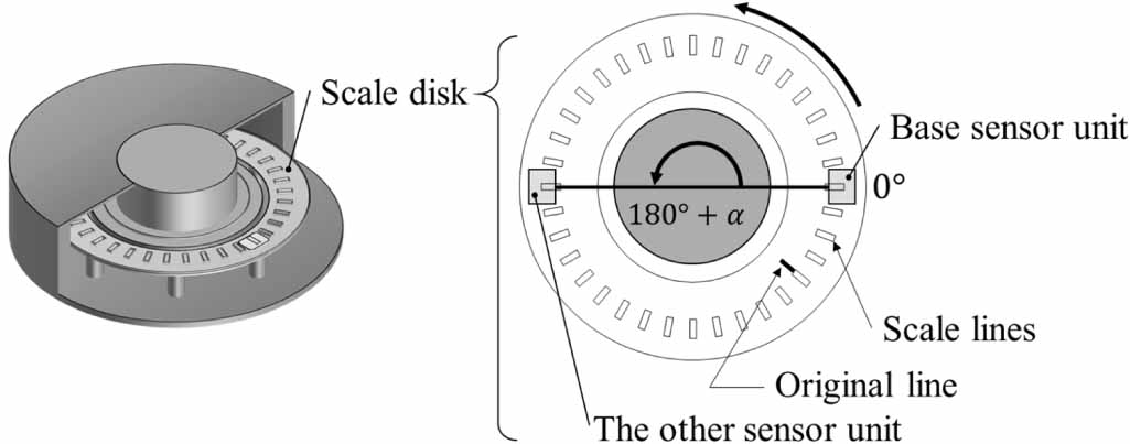
A rotary encoder can measure the full range of angles (0°–360°) and is used to control the rotational position of a shaft [6]. It consists of a disk with scale lines arranged like a protractor scale, which is read by sensor units. As the angle signals of the sensor units include the angle error, the output position differs from the ideal angle position. The angle accuracy of a rotary encoder can be improved by two methods: direct reduction of the angle error factors (such as runout of the main shaft and the eccentricity between the center of the main shaft and the scale disk) using the high performance parts of the rotary encoder, and self-calibration that detects and self-corrects the angle error. The angle accuracy of these methods is 0.1–0.4 arcsecs in each rotation [7, 8]. Further, the angle accuracy of the national standard in Japan using these methods is 0.01 arcsecs [9, 10].
The static angle position is measured by the rotary encoder as described above. However, the angle accuracy of these methods is limited because their calibrations are difficult to be performed on a specific scale line in the static angle position. Therefore, the National Institute of Advanced Industrial Science and Technology (NMIJ/AIST) in Japan has developed an angular indexing apparatus that measures the static angle positions without these methods [11]. The apparatus is applied in the principle of super-high-accuracy angular indexing. However, this principle has not exactly derived the indexing angle because its equations were expressed qualitatively. Therefore, the principle must be quantitatively derived by formulating the angle signal positions, which satisfy the circular closure property [12]. After formulating the angle signal position output by the rotary encoder, we simulate the principle and present its results.
2. Principle
This section formulates the angle signal positions output by the rotary encoder. Based on this formulation, it derives the principle of the super-high-accuracy angular indexing.
At first, the angle signal position output by a rotary encoder is expressed by a mathematical equation.
Figure 1 displays an optical-type rotary encoder. This encoder consists of two sensor units, which are arranged in an angular position with  around the scale disk; the installation error of the sensor units
  denotes the angular misalignment error between the ideal arrangement position of the base sensor units and the other sensor unit. Figure 2 shows the relationships of the angle signal positions output by the sensor units. As shown in figure 2,
  is the ideal angle position and is given as

where  are the numbers of the scale lines, and
  is the total number of scale lines. The counterclockwise direction is taken as the positive direction. Additionally, let
  and
and  be the angle signal positions output by two sensor units, expressed by equations (2) and (3) respectively:


where  and
and  denote the corresponding angle errors.

Figure 1. An optical-type rotary encoder.
Download figure:
Standard image High-resolution image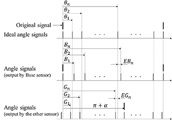
Figure 2. Relationships among the angle signal positions.
Download figure:
Standard image High-resolution imageFigure 3 shows the relationship between the angle errors in two sensor units for a case  and the Fourier components of the phases and their difference. The top panel shows the angle errors indicated by
  and
and  . Moreover, two angle errors coincide at 0° and 360° and sum to zero because they possess the circle closure property [1, 12]. Therefore, any arbitrary function of the angle error can be expanded as a Fourier series because the angle error is the periodic function in one rotation. The bottom panels show the phase of the angle error in each Fourier component and its difference. As indicated in the difference, the phases in the odd-term Fourier components are 180° and the phases in the even-term Fourier components are 0°. Therefore, the phase of the angle error depends on the installation position of the two sensor units. Accordingly, the angle errors
  and
and  can be expressed by equations (4) and (5), respectively:
where  is a complex number and
  is the imaginary unit.
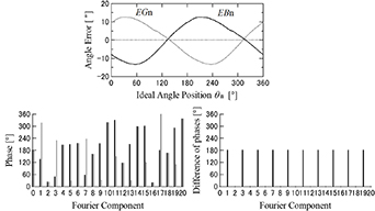
Figure 3. Relationship between the angle errors and their phases. Bottom panels are the Fourier components of the phases.
Download figure:
Standard image High-resolution imageThe respective angle signal positions are then expressed as
Taking the average of equations (6) and (7), the angle signal position output by the rotary encoder is computed as
Secondly, the angle signal positions output by the apparatus shown in figure 4 are expressed by a mathematical equation.
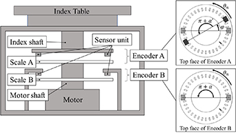
Figure 4. Model of the angular indexing apparatus applied in the principle of super-high-accuracy angular indexing.
Download figure:
Standard image High-resolution imageThe apparatus has two scale disks (Scale A and Scale B) with the same total scale line  , two coaxial independent shafts (index shaft and motor shaft) and two sets of sensor units that are arranged in 180° angular position. Encoder B consists of Scale B and the sensor unit attached to the housing of the apparatus. Encoder A also consists of Scale A and the sensor unit attached to the index shaft that extends below the index table. As indicated in the top face of Encoder A, the sensor units of Encoder A are indexed and rotated in sync with the indexing angle
  of the index table. Moreover, the installation error of the sensor units
  denotes the angular misalignment error between the ideal arrangement position of the base sensor units and the other sensor unit. Figure 5 shows the relationships between the angle signal positions output from the apparatus in figure 4.

Figure 5. Relationship between angle signal positions output by Encoder A and Encoder B in figure 4, and its visual representation.
Download figure:
Standard image High-resolution imageThe sensor units of Encoder B are fixed in the housing of the apparatus. Encoder B outputs the angle signals triggered by its original signal (see figure 2). Therefore, the angle signal positions output by Encoder B are given by  in equation (8).
As shown in figure 5, Encoder A outputs the angle signals triggered by Encoder B's original signal. We first explain the original signal position  output by Encoder A.
  is the angle between the original signal positions of Encoder A and Encoder B, and changes with the indexing angle
  . Therefore,
  is given as

where  is the initial original signal position output by Encoder A at
  . Additionally,
  can be eliminated by calculating more than one value of
  because
  is a constant value.
Next, we explain the relationship between  and angle signal output by Encoder B. As indicated in figure 5,
  is the ideal angle signals of Encoder B and can be expressed as

where  is the positive integer indicating the number of the scale line output by Encoder B after Encoder A detects its own original signal. Then, replacing
  with the scale number expanding to a decimal range, we get

Therefore, the number of scale line  can be expressed as

where  is the floor function.
Accordingly,  is a function of the indexing angle
  and is specifically given by

We now explain the angle signal positions  output by Encoder A.
  can be derived from the following three facts and is expressed by equation (14).
 takes the form of equation (8) because the sensor units of Encoder A are installed in diametrically opposite positions as in Encoder B.
- The phase of the angle error in changes with the indexing angle of the index table because the installation positions of the sensor units in Encoder A are indexed synchronously with .
- Like the original signal position of Encoder A, includes a term because Encoder A outputs the angle signals triggered by Encoder B's original signal:


where  is a complex number.
Finally, deriving the indexing angle  of the index table. The angle signal positions of Encoder A and Encoder B are given by equations (14) and (8), respectively. The indexing angle
  can be directly calculated from
  and
and  by equation (10) because
  of equation (10) is the function of
  .
.  can be calculated by counting the z angle signals detected by Encoder A between the original signals of Encoder A and Encoder B. Next,
  is obtained directly as follows:
- (i)

- (ii)Taking the average difference over the scale lines, equation (15) becomes

where  and
and  are the offsets of the angle errors.
These offsets are constants and independent of the indexing angle  . Equation (16) provides a direct derivation of
  because the offsets are eliminated for any
  .
.
3. Simulation
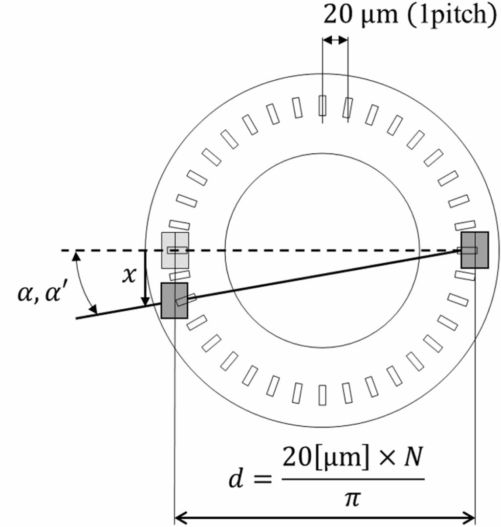
To confirm that the offsets in equation (16) indeed cancel and that equation (16) matches equation (13), simulations were carried out under the conditions shown in table 1. As indicated in table 1, the simulation ranges and its steps are determined at the values that are confirmed to calculate less than the resolution of the conditions. The total number of scale lines are the same values in the two simulation, and then the steps between the scale lines are 20 μm. The initial indexing angles are zero for ease during simulations. The installation errors  and
and  are determined by values that are calculated using the case of the misalignment with 200 μm and 400 μm in the x direction, respectively, as shown in figure 6. Figure 7 plots
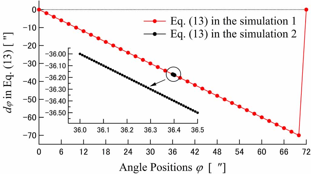
  calculated from equation (13) using the parameters of the simulation conditions.
Table 1. Simulation conditions.
| Simulation 1 | Simulation 2 | |
|---|---|---|
Simulation range of  (arcsecs) (arcsecs) |
 (1 step) (1 step) |
 |
| Step width (arcsec) | 2 | 0.01 |
| Total number of scale lines N | 18 000 | 18 000 |
Initial indexing angle  |
0 | 0 |
Installation error  |
0.1 | 0.1 |
Installation error  |
0.2 | 0.2 |

Figure 6. Calculation of the installation errors.
Download figure:
Standard image High-resolution image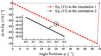
Figure 7. Simulation result of equation (13).
Download figure:
Standard image High-resolution imageAs indicated in figure 7, the horizontal axis is angle position  as shown in table 1 and the vertical axis is the
  calculated from equation (13). Moreover, equation (13) is confirmed to have the proportional relationship regarding the angle position
  as same as its theory.
The coefficients  and
and  in equations (8) and (14) were computed by equations (17) and (18) respectively, and their values are listed in table 2. Figure 8 plots the simulated results of equations (17) and (18) using the parameters of table 2:


Table 2. Angle error parameters calculated by equations (17) and (18).
Period  |
 |
 |
||
|---|---|---|---|---|
 ('') ('') |
 (°) (°) |
 ('') ('') |
 (°) (°) |
|
| 0 | 10 | 0 | 20 | 0 |
| 1 | 50 | 30 | 70 | 10 |
| 2 | 40 | 60 | 60 | 40 |
| 3 | 30 | 90 | 50 | 70 |
| 4 | 25 | 120 | 45 | 100 |
| 5 | 20 | 150 | 30 | 130 |
| 6 | 15 | 180 | 25 | 160 |
| 7 | 10 | 210 | 20 | 190 |
| 8 | 5 | 240 | 15 | 220 |
| 9 | 2 | 270 | 10 | 250 |
| 10 | 1 | 300 | 5 | 280 |

Download figure:
Standard image High-resolution imageFigure 8 plots the real-part and the imaginary-part in each equation (17) and equation (18) because equations (17) and (18) are defined as the complex number. To plot the complex number to figure 8, we can obtain the relationship between the amounts of the amplitude in each period of equations (17) and (18).  and
and  in table 2 are used the values that decrease toward the higher periods in the lower periods range as same as the real angle error detected by the rotary encoder. Specifically, the eccentricity as the angle error factors gives the large influence to one period component in an angle error. Moreover, the runout gives the influence to the lower periods range. The scale disk also gives same influence as the runout.
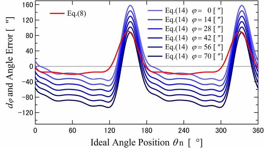
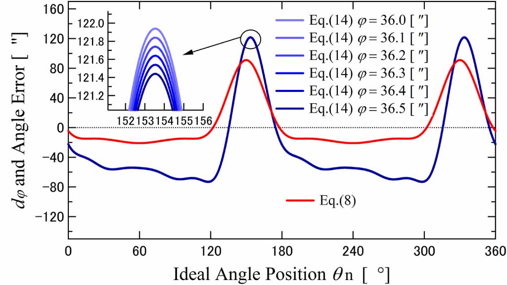
Figure 9 plots the  and the angle error calculated from equations (8) and (14) for various
  in simulation 1. Figure 10 also plots the
  and the angle error calculated from equations (8) and (14) for various
  in simulation 2. As indicated in the two figures, the horizontal axis is the ideal angle position and the vertical axis denotes the angle error and equation (13) from the ideal angle position in equations (8) and (14). Moreover, equation (14) has the different offsets about various
  and includes not only even-order periodic components of the angle error but also odd-order periodic components because two simulations have considered the installation error of the sensors.


Download figure:
Standard image High-resolution image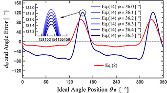

Download figure:
Standard image High-resolution imageFigure 11 plots the  in equation (15) calculated by approach (i) in section 2 under simulation 1, and figure 12 also plots the
  in equation (15) calculated by approach (i) in section 2 under simulation 2. Then, the horizontal axis is the ideal angle position and the vertical axis is the difference values between equations (8) and (14). Moreover, equation (15) also has the different offsets about various
  . As the actual analysis scene, we can first analyze equation (15) indicated in figures 11 and 12, and at second calculate the indexing angle
  .
.
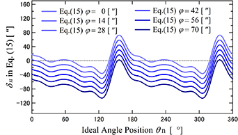
Figure 11. Simulation results of equation (15) for various  in simulation 1.
Download figure:
Standard image High-resolution image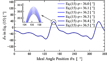
Figure 12. Simulation results of equation (15) for various  in simulation 2.
Download figure:
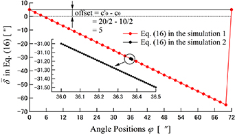
Standard image High-resolution imageFigure 13 shows the  in equation (16) calculated by approach (ii). The vertical axis shows the average values for equation (15) in various
  .
.
Figure 13. Simulation results of equation (16) by approach (ii).
Download figure:
Standard image High-resolution image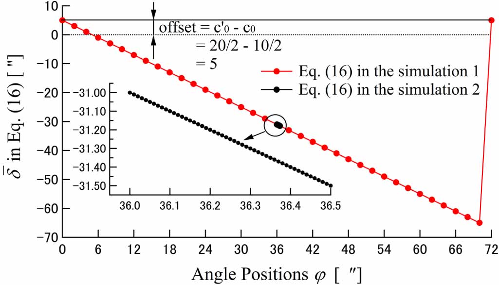
Comparing the simulation results of figures 7 and 13, we confirm that equations (13) and (16) are similar in sign. Moreover,  in equation (16) indicated in figure 13 decreases in proportion to the indexing angle
  between adjacent scale lines as same as figure 7. Additionally, equation (16) clearly describes the offset and is consistent with the theory. This offset can be eliminated in the analysis because the all values calculated using equation (16) are shifted. Therefore, we can obtain equation (13) directly through approaches (i) and (ii) in section 2. Additionally, we can match
  in equation (10) to the indexing angle
  shown in table 1 through equations (1) and (16). Accordingly, the principle of the super-high-accuracy angular indexing is validated and quantitatively derived. Moreover, the angular indexing accuracy is expected to improve to 0.01 arcsecs because it is not limited by the resolution and accuracy of the rotary encoder; moreover, it eliminates the angle error accompanying the angle signals.
4. Conclusion
Highly accurate measurements of the indexing angle of an index table are necessary for improving the processing accuracy of machining tools. In previous research, the indexing angle was measured by optical methods using an interferometer. Here we developed a special optical method that measures this angle using two rotary encoders. We call this method the principle of super-high-accuracy angular indexing. This paper presented a formal derivation of the principle and validated it in a simulation study. The following conclusions were drawn from the results:
- The principle was derived by formulating the angle signal positions' output by the rotary encoders.
- This formulation was expressed as a Fourier series expansion of the angular errors of the installation positions of the sensor units built into the rotary encoder. The errors have circular closure.
- The simulation results were exactly matched. Therefore, the simulation confirmed that the mathematical equation quantifies the principle of super-high-accuracy angular indexing.
- The characteristics of the principle is that it can remove the angle error having the angle signals' output by a rotary encoder.
- The advantage of the principle is that it can measure all indexing angles in theory. Its disadvantage is that it cannot measure in real-time because the measurement needs one rotation.
In future work, we will compare the theoretical values with actual values.