Linearity of photovoltaic devices: quantitative assessment with N-lamp method

The electrical performance of photovoltaic (PV) devices is measured under natural or simulated sunlight. One of the most crucial and difficult measurements is that of the incident irradiance [1]. This is typically done with a PV reference device, usually a solar cell. These devices are normally calibrated at standard test conditions (STC), which amount to 1000 W m⁻² total irradiance under a defined spectral irradiance (IEC 60904-3 [2]) and PV device junction temperature of 25 °C. The calibration value at STC is taken as the reference point, and usually this is the only data point available from the calibration of a PV reference device. While the most common testing of electrical performance of PV devices is also made at STC, the performance at other irradiances is of interest in the context of energy rating (IEC 61853-1 [3]). In the latter standard the power matrix requires measurements in the irradiance range from 100 W m⁻² to 1100 W m⁻². Normally the reference device is not calibrated separately at these different irradiances spanning roughly one order of magnitude. Rather a simple proportionality between incident total irradiance and short-circuit current output of the reference device is assumed. This is called linearity of the PV (reference) device and methods for the linearity measurement are addressed in a dedicated standard (IEC 60904-10 [4]) (hereafter linearity standard). Several other standards of the IEC 60904 series and IEC 60891 [5] call upon the linearity standard, essentially stating (explicitly or only implicitly) that for linear PV devices the proportionality calculation can be applied. However, there are two major problems with the current version of the linearity standard. The first being that the definition of linearity considers a generic linear relationship between short-circuit current and irradiance whereas it should test for the direct proportionality of the two parameters. Secondly, linearity as defined by the standard is only a pass/fail test with an arbitrary limit of 2% deviation. This implies that by using a PV reference device which is classed as linear according to the current version of the linearity standard could result in deviations of up to 2% in the measurement of the incident irradiance in electrical performance measurements of PV devices. This is outdated and undesirable as state-of-the-art measurement have a measurement uncertainty (UC) for incident irradiance well below 1% (with the lowest available of 0.25% [6]) in order to achieve uncertainties for the maximum power of PV modules in the range of 1% to 2%.

A similar problem arises in photometry, where the linearity of photomultipliers and photodiodes has to be determined. This is most commonly done with methods based on the flux addition principle, such as the two-lamp method. Essentially, the output of a detector is measured using two optical fluxes separately as well as their sum. A comparison of the measured outputs yields information about the linearity of the detector assuming that the optical fluxes add (for details see below). This does not require any reference device, and therefore can be deemed a primary method for determination of detector linearity.

The flux addition principle (also called superposition method) [7] has been implemented traditionally by using one light source and providing two (or more) effective light sources using for example apertures of defined size [7–10]. This was mainly because the light source has to have a high temporal stability, which requires special stabilising circuitry making each light source expensive, and therefore the number of light sources has been minimized (one source) [7]. In fact there are few examples of using multiple sources and those requiring more than two seem to have been abandoned [7], with only methods using two sources (hence the two-lamp method) being used.

The two-lamp method can be applied over a wide irradiance range, typically several orders of magnitude. Various implementations can be found in the literature [11, 12] with sophisticated data analysis methods based on matrix algebra. Essentially the output of the detector with respect to the irradiance is modelled by a polynomial function [13, 14]. Each measurement gives a set of equations which can be used to determine the coefficients in the function. Typically, there are many more measurements than coefficients and therefore the problem is mathematically overdetermined and the coefficients are determined minimizing the deviations (sum of squares).

The two-lamp method provides linearity information for an interval of irradiances spanning a range of a factor of two. Information over larger ranges can be obtained by combining several measurements such that the lower irradiance of the next interval equals the combined of the previous, i.e. going towards higher irradiance (or the combined irradiance of the next interval equals single of the previous, i.e. going towards lower irradiance) [9, 15]. However, no information is obtained within a single irradiance interval. This is advantageous in applications where information over a large range of irradiances (typical 5–6 orders of magnitude) is sought, as it limits the number of measurements required for spanning such a large range. However, in PV the linearity over an irradiance range of one order of magnitude is of interest, preferably with detailed information within this range, but the two-lamp method only yields 3 to 4 data points.

The two-lamp method was introduced in PV by Emery (NREL) who described a suitable apparatus and procedure [16, 17]. It was designed as a qualitative test [18] and provides a series of data points for specific irradiance intervals without giving information about the linearity over the entire irradiance range. Based on the results presented [16], it was clear that the data from the two-lamp method could not be compared directly with the results of the differential spectral responsivity (DSR) method [19]. Nevertheless both methods were included in the linearity standard IEC 60904-10 [4] as equivalent, but it is conceivable that the two different methods will give opposing answers as to whether a PV device is linear or not; in fact the device tested here is one example of such a case [20]. Recently a simple data analysis scheme for the two-lamp method was proposed which provides this quantitative information about the non-linearity (NL) over the full range of measured irradiances [20], combining local non-linearities (one measurement) to a global NL (over the entire measured range). This allows comparing, over the entire irradiance range of interest, the results of the two-lamp method to those from other methods, for example from the DSR [21]. However, this does not solve the shortcoming of the two-lamp method of not providing information within an irradiance interval of a factor of two. This can only be addressed by using more/multiple light sources, in general named N-lamp method. Historically they seem to have been abandoned probably due to high investment, both in equipment (multiple lamps) as well as number of measurements [7]. However, it had already been pointed out that this is also accompanied by a lower uncertainty [10]. Therefore, the use of the flux addition principle with multiple (in this work: eleven) lamps is ideally suited to the application in PV where linearity information over a limited range (one order of magnitude) with higher detail and low uncertainty is required. One aspect mainly overlooked in the literature is that the N-lamp method gives more information within a spanned irradiance range. Normally the parameters examined are the total range spanned, the number of measurements required and the uncertainty of the linearity [10].

The current work aims to improve on these shortcomings in several ways. Firstly a framework for quantitative information about the linearity of the short-circuit current versus incident irradiance for PV devices is developed based on the physical principle of proportionality between them. The NL is treated as a quantitative parameter and no arbitrary limits for pass/fail are required. Based on this an explicit correction can be applied for correcting the irradiance as determined from the short-circuit current from a non-linear PV device. Then the mathematical framework for obtaining this information from an N-lamp method (here N  =  11) is described. Finally experimental results are presented by applying the method to a PV reference cell which has a certain degree of NL. The uncertainty of the linearity information is derived and presented.

Device under test (DUT)

Solar simulator and measurements

The large-area steady-state solar simulator APOLLO at the European Solar Test Installation (ESTI) was used to perform the measurements. The simulator consists of 11 nominally identical Xenon high-pressure arc-discharge lamps which provide simulated sunlight over an area of 2 m by 2 m with class AAA (IEC 60904-9 [24]). Each lamp illuminates the entire target plane by superimposing multiple images of the source [25]. After switch-on and a warm-up time of 30 min the irradiance provided by the lamps is stable according to IEC 60904-9 (detailed data on stability are presented with the results). The DUT was placed slightly ahead of the usual target plane such that a total irradiance of 1100 W m⁻² was reached, each lamp contributing about 100 W m⁻² on average. In this way the range from 100 W m⁻² to 1100 W m⁻² was covered in steps of approximately 100 W m⁻² by using a suitable number of lamps.

Each of the 11 lamps is equipped with a shutter, which can be individually opened or closed from the remote control computer and which thereby allows the light generated by single lamps to reach the DUT or not. It takes about 20 s for the shutter to move from one position to the other. Additionally, between the lamps and the DUT a curtain is installed that can be remotely opened and closed in less than 2 s and is useful to shield the DUT while shutters are operated. The DUT is mounted on a Peltier cooler with feedback regulating its temperature to (25  ±  0.5) °C even when the irradiance is rapidly changing due to opening or closing of lamps.

For the two-lamp method measurements, the short-circuit current of the DUT is amplified by a proprietary transimpedance amplifier maintaining the device in short-circuit conditions. The output voltage was measured by a calibrated digital storage oscilloscope, whose voltage scale is adjusted for each acquisition run in order to accommodate the highest expected signal from the DUT. Once the data acquisition is started, the lamps are opened and closed while a trace is recorded. Typically, each condition of illumination is held for one minute, showing a plateau in the data versus time. In the data analysis the average value of each plateau is determined by simple arithmetic averaging. The background stray light inside the darkroom is measured (with room lights off, all simulator lamps on, all lamp shutters closed and the curtain open) and subtracted from each individual measurement. However, the background is more than three orders of magnitude smaller than the signal induced by a single lamp and could therefore simply be neglected.

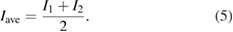
Using the individually controlled shutters, suitable sub-sets of the 11 lamps total were used, examples are shown in figure 1. The two-lamp method using lamp #1, lamp #2 and both of them together (#1 and #2) (figure 1(a)) and the seven-lamp method with individual signals from each of the seven lamps as well as from them combined (figure 1(b)) would each yield one data point for NL assessment. The full measurement with 11 lamps consists of two traces (figure 1(c)) (acquired one after the other), the first showing the signals from all eleven lamps, then ten lamps and so forth down to one lamp and the second recording the signals from all eleven lamps individually. This 'staircase' measurement yields a full set of data points to determine the NL over the entire range (see below).

Zoom In Zoom Out Reset image size

Linearity

For a perfectly linear PV reference device the short-circuit current I_SC output is proportional to incident irradiance, so that

$$\begin{align} \newcommand{\e}{{\rm e}} \displaystyle {{I}_{{\rm SC}}}=\frac{{{I}_{{\rm STC}}}}{1000~\,{\rm W}\,{{{\rm m}}^{-2}}}G=\frac{CV}{1000\,{\rm W}\,{{{\rm m}}^{-2}}}G\nonumber \end{align} \tag{ 1 }$$

where the expected short-circuit current I_SC is calculated based on incident irradiance G and the calibration value CV of the PV reference device equals the short-circuit current at STC, I_STC. By using G_ref instead of 1000 W m⁻² it can easily be generalized to calibration values at other conditions. A practical reference device might exhibit a NL which is the deviation of the measured short-circuit current I_meas from that expected according to equation (1), at some irradiance G other than STC:

$$\begin{align} \newcommand{\e}{{\rm e}} \displaystyle NL\left({{I}_{{\rm meas}}} \right)=\frac{{{I}_{{\rm meas}}}-{{I}_{{\rm SC}}}}{{{I}_{{\rm SC}}}}=\frac{{{I}_{{\rm meas}}}}{CV}\frac{1000\,{\rm W}\,{{{\rm m}}^{-2}}}{G}-1.\nonumber \end{align} \tag{ 2 }$$

By this definition the reference point at STC has no NL, i.e. NL(CV)  =  0.

In measurements of PV device performance the incident irradiance is calculated from equation (1) using the measured short-circuit current I_meas of the reference cell as I_SC. If quantitative information about the NL according to equation (2) is available for the range of I_meas (i.e. G) of interest, the irradiance corrected for the NL can be obtained as:

$$\begin{align} \newcommand{\e}{{\rm e}} \displaystyle G=\frac{1000\,{\rm W}\,{{{\rm m}}^{-2}}}{CV}\frac{{{I}_{{\rm meas}}}}{1+NL\left({{I}_{{\rm meas}}} \right)}=\frac{1000\,{\rm W}\,{{{\rm m}}^{-2}}}{CV}\frac{{{I}_{{\rm meas}}}}{R\left({{I}_{{\rm meas}}} \right)}\nonumber \end{align} \tag{ 3 }$$

with a correction factor R(I_meas). Please note the similarity of equation (3) with that for spectral mismatch correction in IEC 60904-7 [26]. Furthermore, equation (3) can be used to convert NL information as a function of I_meas to the irradiance scale, i.e. as a function of G, by simply calculating the irradiance corresponding to a given I_meas.

Below, it will be shown how to obtain the correction factor R from the two- and N-lamp methods.

Two-lamp method

In the two-lamp method lamps #1 and #2 providing (roughly) equal irradiance (G₁ or G₂) are used to illuminate the PV device by each lamp singularly and with both lamps together (irradiance G₁₂) and recording I_meas in each case. The background I_room due to stray light has to be measured separately and subtracted from each individual measurement. In the following, it is assumed that this is done for all measurements.

For a perfectly linear device the sum of the two individually measured photocurrents I₁ and I₂ will be equal to the photocurrent I₁₂ measured under full irradiance, so that the ratio R:

$$\begin{align} \newcommand{\e}{{\rm e}} \displaystyle R({{I}_{12}})=\frac{{{I}_{12}}}{{{I}_{1}}+{{I}_{2}}}\nonumber \end{align} \tag{ 4 }$$

equals the value 1. In practical devices R differs from 1 and equation (4) gives the relative correction factor in equation (3) at the short-circuit current I₁₂ with respect to (the reference point) I_ave [8]:

$$\begin{align} \newcommand{\e}{{\rm e}} \displaystyle {{I}_{{\rm ave}}}=\frac{{{I}_{1}}+{{I}_{2}}}{2}.\nonumber \end{align} \tag{ 5 }$$

The reference point is assigned the value of R(I_ave)  =  1. The relative correction factor at the short-circuit current I_ave with respect to I₁₂ is just the inverse, i.e. $R\left({{I}_{{\rm ave}}} \right)=\frac{{{I}_{1}}+{{I}_{2}}}{{{I}_{12}}}$ and R(I₁₂)  =  1. The NL between the two is simply the deviation of R from the value of 1, again analogous to spectral mismatch correction in IEC 60904-7 [26] which is also typically a value near 1 and the deviation from this is called the spectral mismatch error.

In the two-lamp method further measurements are taken such that the individual induced I_meas of a single lamp equals that of both lamps in the previous step (going up in irradiance) or such that the induced I_meas of both lamps equals that of a single lamp in the previous step (going down in irradiance). This can be achieved by varying lamp intensity (varying lamp power, use of mesh or neutral density filters or precision apertures of varying sizes as well as distance to the sources). The overall correction factor for a larger range is then simply given by the product of the correction factors for each single step in irradiance [9, 15]. Correction factors for intermediate values of I_meas can be obtained by suitable interpolation between the measured data points R. However, such interpolation assumes a linear (or other, if reasonable from the overall data set) variation of linearity within an interval, as in the two-lamp method there is not (and cannot be) any information inside an interval of factor two. The N-lamp method presented below overcomes this fundamental problem.

N-lamp method

The extension to the N-lamp method is obtained by measuring all N (here 11) lamps singularly and then measuring combinations (at least one each) of two, three, ..., N lamps. In this way, the irradiance range from one lamp (here 100 W m⁻²) to N lamps (here 11 corresponding to 1100 W m⁻²) is covered in roughly equal steps (here of 100 W m⁻²). The assumption, which is valid in our case, is that all N lamps give about the same irradiance level on the test plane. All measurements are referenced to a single point, the average irradiance of the lamps (around 100 W m⁻²):

$$\begin{align} \newcommand{\e}{{\rm e}} \displaystyle {{I}_{{\rm ave}}}=\frac{\sum\nolimits_{i=1}^{n}{{{I}_{i}}}}{n}\nonumber \end{align} \tag{ 6 }$$

so that all points are referring to roughly the same reference points I_ave. The quantity n represents the number of lamps combined to achieve the irradiance level from 100 W m⁻² to 1100 W m⁻². The correction factor with respect to this reference point is then

$$\begin{align} \newcommand{\e}{{\rm e}} \displaystyle {{R}^{\prime}}({{I}_{n}})=\frac{{{I}_{n}}}{\sum\nolimits_{i=1}^{n}{{{I}_{i}}}}\nonumber \end{align} \tag{ 7 }$$

using the prime to indicate that this is not the final correction factor. In fact the function R' has to be normalized by dividing through the value of R'(CV) (obtained by suitable fitting of a function to R')

$$\begin{align} \newcommand{\e}{{\rm e}} \displaystyle R(I)=\frac{{{R}^{\prime}}(I)}{{{R}^{\prime}}(CV)}\nonumber \end{align} \tag{ 8 }$$

such that R(CV)  =  1.

Linearity with N-lamp method

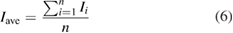
Based on the trace shown in figure 1(c) the data points of the function R' were calculated with equation (7) (figure 2). For this, all possible combinations of n lamps (from n  =  2 to n  =  11) were used. For each of them the reference point R'(I_ave)  =  1 is referring to a slightly different value of I_ave, so that the leftmost point actually consists of ten individual points, which however overlap almost perfectly.

Zoom In Zoom Out Reset image size

Next, a quadratic function was fit to the R' points and the value of R'(CV) determined and used for normalization according to equation (8). The points R were so calculated, which refer to the CV of the device.

UC analysis

The UC analysis (see table 1) is based on the already established UC analysis [1] of I–V curve measurements on the APOLLO solar simulator. Most components of the I–V's UC analysis are not relevant for the linearity UC because they cancel out in the two-lamp method, since they are common to all measurements (e.g. Orientation of DUT). In particular the spatial non-uniformity of the irradiance is irrelevant during the assessment of linearity of a single reference cell (for more details see discussion). The remaining components are the UC of the data acquisition system and of the transimpedance amplifier as well as contributions connected to DUT temperature (temperature indicators, deviation of measurement conditions from 25 °C and difference in temperature between temperature sensor and p-n junction). Furthermore, the NL of the transimpedance amplifier and the lamp stability were added as additional components here for the specific case of linearity assessment. They are not normally relevant during I–V curve measurement because there the irradiance is measured by a reference cell for each data point of the curve and then corrected point by point. For the two- or N-lamp methods, instead, the stability of the lamps between the measurement with the single lamp and the one in which it is used in combination with other lamps is relevant. This component was deduced from repeated measurements of the same lamp. The average standard deviation for the lamp stability (repeatability) is 0.1% (k  =  1) or less for most lamps, but it ranges up to 0.2% for some lamps (two or three). A value of 0.15% (k  =  1) is used for lamp stability in the following. This is a conservative estimate, because, when using more than one lamp, it is likely that at most one of them has the higher UC of 0.2%. Therefore, only in the case of two lamps (one having 0.1% and one having 0.2%) is the overall UC (0.223%) slightly larger than assuming two lamps (having each 0.15%) yielding 0.21%. For all other n, starting with n  =  3, the estimated uncertainty based on all lamps having an uncertainty of 0.15% is larger than assuming one lamp with 0.2% and all other with 0.1%. This also remains true when two lamps out of five or more have the higher UC of 0.2%. Table 1 summarizes the UC for the measurement of the short-circuit current induced in the DUT by a single lamp, yielding an expanded combined UC (UC₁) of 0.30%.

Table 1. UC budget analysis for linearity measurement.

Standard uncertainty component	Standard UC	Distribution	Short-circuit current
	Type (A/B)	Gaussian/rectangular	%
Data acquisition system	B	G	±0.023
Trans impedance amplifier for reference cell	A	G	±0.006
Linearity of trans impedance amplifier	A	G	±0.015
Combined standard electrical UC			±  0.03
Temperature indicators	B	R	±0.003
Measurement conditions: DUT temperature	B	R	±0.014
Difference p-n junction/sensor for DUT	B	R	±0.014
Combined standard temperature UC			±  0.02
Non-uniformity of spatial irradiance	B	R	±0.000
Orientation of device under test and reference device	B	G	±0.000
Alignment of device under test and reference device	B	R	±0.000
Combined standard optical UC			±  0.00
Calibration of reference device	A	G	±0.000
Determination of spectral mismatch correction factor	B	G	±0.000
Reference cell drift	A	G	±0.000
Combined standard reference device UC			±  0.00
Standard solar simulator lamp stability UC	A	G	±  0.15
Combined standard UC			±0.15
Expanded combined UC (k  =  2): UC1			±  0.30

As evident from table 1 the overall uncertainty is entirely dominated by the stability of the lamps, which is due to random fluctuation. Assuming that the irradiance fluctuations of various lamps are uncorrelated, the absolute UC will increase with the square root of n, but since the irradiance increases proportionally to n, the relative UC (all UCs used here are relative UCs) of the irradiance produced by n lamps is simply

$$\begin{align} \newcommand{\e}{{\rm e}} \displaystyle {\rm U}{{{\rm C}}_{n}}\left(k=2 \right)=\frac{1}{\sqrt{n}}{\rm U}{{{\rm C}}_{1}}(k=2)\nonumber \end{align} \tag{ 9 }$$

with UC₁ (k  =  2)  =  0.30% (table 1). This is true for both cases, where a mathematical sum is taken of individual measurements of n lamps as well as when all n lamps illuminate the DUT simultaneously. Therefore, the UC of R' (equation (7)) is:

$$\begin{align} \newcommand{\e}{{\rm e}} \displaystyle {\rm U}{{{\rm C}}_{{{R}^{\prime}}}}\left(k=2 \right)=\sqrt{\frac{2}{n}}{\rm U}{{{\rm C}}_{1}}(k=2)\nonumber \end{align} \tag{ 10 }$$

with UC₁ as before. On this basis, the UCs shown in figure 2 were assigned for each data point R' with the exception of the reference points (multiple points around 12 mA), which do not have any UC by definition. The size of UC decreases from left to right with increasing number of the lamps considered in the calculation for the data point. The UC for the normalized data points R were then calculated by assigning an UC of 0.14% to the value of R'(CV) (average UC of neighbouring data points) and calculating the combined UC by usual propagation.

The disadvantage of the approach so far is that 21 measurements are required for the full set which takes typically 40–50 min. As the lamp stability is the main UC component, it was investigated whether the stability is higher for measurement times shorter than that. This is indeed the case, with lamp stability standard deviation of 0.07% (k  =  1). This offers the possibility to do measurements (for example by the two-lamp method) with lower UC.

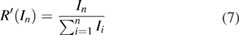
This was investigated in more detail by repeating measurements for the two-, three-, five- and seven-lamp method (figure 3) and served to establish whether the experimental variation of repeated measurements is consistent with the UC estimate made (equation (10)). Table 2 additionally also lists the experimental variability of a number of combinations using the two- and three-lamp method where each 'virtual' lamp is composed of a set of lamps. In the last two columns the experimentally observed variability (UC_exp, calculated as twice the standard deviation) is compared to the UC expected from the calculation above (UC_calc, based on equation (10)). Here, the value of 0.07% (k  =  1) was used for the lamp stability, as determined from a number of repetitions within the shorter time frame typical of the time required for these measurements. Replacing in table 1 the value  ±  0.15% of the Standard Solar Simulator Lamp Stability UC with the value  ±0.07% derived experimentally, the Expanded Combined UC (k  =  2): UC₁ in the bottom line of table 1 becomes  ±0.16% instead of  ±0.30%. For the 11-lamp method there is only one data point (table 2).

Zoom In Zoom Out Reset image size

Table 2. Experimental data on R' repeatability compared to the analytical prediction. From the standard deviation (SD) of the data the experimental UC_exp is calculated and compared to the UC_calc according to equation (10). The experimental UC_exp of the average R' is reported in the last column. For 11 lamps there was only one data point.

Method	n	Average Iave mA	Average In mA	Average R'	SD (R') (k  =  1)	Repetitions	UCexp R' (k  =  2) %	UCcalc R' (k  =  2) %	UCexp ave R' (k  =  2) %
2 * 1	2	12.62	25.37	1.004 97	0.000 69	21	0.136	0.160	0.030
3 * 1	3	12.40	37.51	1.008 41	0.000 83	8	0.166	0.131	0.059
2 * 2	4	24.77	49.84	1.00 610	0.000 51	12	0.102	0.113	0.029
5 * 1	5	12.39	62.78	1.013 37	0.000 37	11	0.074	0.101	0.022
2 * 3	6	37.43	75.35	1.006 57	0.000 77	10	0.154	0.092	0.049
3 * 2	6	25.04	75.89	1.010 09	0.000 48	8	0.096	0.092	0.034
7 * 1	7	12.23	87.15	1.017 97	0.000 41	4	0.080	0.086	0.040
2 * 4	8	49.68	100.07	1.007 07	0.000 35	9	0.070	0.080	0.023
3 * 3	9	37.48	113.77	1.011 93	0.000 74	7	0.146	0.075	0.055
2 * 5	10	62.69	126.32	1.007 48	0.000 31	7	0.062	0.072	0.023
11 * 1	11	12.41	139.44	1.021 62	NA	1	NA	0.068	NA

It is seen that in general the predicted UC agrees well with the experimentally observed, with some exceptions. They are attributed to the fact that some lamps are noticeably less stable than others. They increase the experimentally observed variability beyond the estimate made by the analytical expression.

In the following the average values of R' will be used, with the respective UC for the mean, based on the experimentally observed standard deviation divided by the square root of the number of repetitions, except for the single data point for n  =  11 which will be assigned the calculated UC. The various measurements can now be combined, for example from the (average) measured R' for two lamps (1.004 97) and four lamps (using two sets of two lamps each, i.e. the two-lamp method with lamps #1 and #2 made of two lamps each) (1.006 10) the value of R' for four lamps (1.011 10  =  1.004 97 * 1.006 10) can be calculated. The uncertainty of the product is determined from the UCs of the two factors by usual propagation.

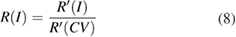
Combining all the information, we can calculate the R' at all intensities and then normalize as before, with UC of 0.05% for the value of R'(CV) (average UCs of neighbouring data points). In figure 4 the final combined function R is compared with the results presented above (figure 2). The UCs of the combined results are noticeably lower, due to the repetition and averaging of several measurements (corresponding also to higher effort). Both results agree well within their respective uncertainties. Also, the double data point at n  =  6 (i.e. triangles at about 600 W m⁻²) for the combined results, based on measurements with two sets of three lamps and three sets of two lamps respectively, agree with each other. From that, it can be also derived that the method is sensitive to the slight difference between the two groups of six lamps used for the two separate sets of measurements.

Zoom In Zoom Out Reset image size

The determination of the NL of a PV reference cell with the N-lamp method was presented including an analysis of the measurement UC and its experimental verification through repeated measurements. In the 11-lamp method the uncertainties ranged from 0.14% to 0.33%, which is significantly lower than the observed NL deviation of more than 2% over the irradiance range investigated. As the dominating component of the UCs (lamp stability) is of statistical nature, the UCs were verified by repetitive measurements. This showed agreement with the analytical predictions and was used to reduce the range of UCs to (0.06%–0.14%) simply by using the average from several equivalent measurements. The results from both approaches agreed within their respective UCs.

During the extensive measurements for this work, it was noticed that some lamps were significantly less stable than others. After a maintenance service, this condition changed in the sense that other lamps were somehow affected, but the individual lamps instability was not entirely eliminated for all of them. No special effort was made to avoid the less stable lamps, especially at the beginning of the campaign, and in particular for those measurements requiring a large number of lamps this would not have been possible anyway. The partly observed variability larger than expected is attributed to this cause. Therefore, only the UCs based on statistical evaluation rather than on analytical prediction were used as they are deemed to be more realistic.

The UCs of the normalization factor were simply estimated as similar to the UC of neighbouring data points. This could potentially be improved by using the UC as determined from the fit. The fit itself could be improved by using the UCs of the single data points as weighting factor, similarly as has been already standardized for linear fits [27]. However, this would make the procedure mathematically much more complex without significant reduction in the resulting UCs. Therefore, the simple approach here was preferred, which is also conservative.

Another approximation made is that the multiple reference points (figure 2) at 12 mA, coming from measurements with different groups of n lamps (with n from 2 to 11), are treated as being essentially at the same I_ave when in reality the latter varies by about  ±4%. From the fit it was estimated that this corresponds to a contribution to the UC that is ten times smaller than the assigned UC and therefore negligible, again in the perspective of simplification.

Spatial non-uniformity of the irradiance and spectral match are secondary factors in the determination of NL. Spectral match may be relevant if the NL is spectrally selective, i.e. sensitive only in certain wavelength bands and not in others. Spatial non-uniformity of irradiance together with spatially inhomogeneous sensitivity of the DUT is only relevant when the PV devices under test have series-connected cells, such as in a PV module. The first cannot in principle be determined by integral methods such as the N-lamp method, but it would require the application of spectrally-selective methods (e.g. DSR [19]). The second would require a separate analysis of the DUT by spatially-resolved methods, which is beyond the scope here, in particular as we are analysing a single PV reference cell. However, by using a solar simulator of class AAA, the spatial non-uniformity is limited to 2% and probably much less for the relatively small DUT investigated here. The latter can be assumed valid for all the irradiance levels spanned in this study, although some degradation of the non-uniformity was observed on the entire test plane when changing from 11 to 1 lamp [25]. Also, the spectral mismatch is contained as the method used to change the irradiance does not involve changing the power of the lamps (which is known to modify their spectral irradiance). In fact, the conditions during the linearity assessment here were very similar to those present during I–V curve measurements (also at variable irradiance), where the DUT would be used as reference device to determine the incident irradiance. Therefore, the linearity determined in this way is perfectly suited for the use of the DUT as reference device, whereas the investigation of potential spatial and spectral effects within the DUT would be of more academic interest (at least for PV solar cells and non-significantly changing spectra).

The evolution of measurement technology for assessment of PV devices, including the purpose of evaluating them under very different environmental conditions, has made it mandatory to treat linearity of PV reference devices not any more in a simplistic way (pass/fail), but to use the approach presented here which gives full quantitative information including a correction procedure for the irradiance (equation (3)). Obviously such quantitative correction has inherent uncertainties, as detailed above. However, for the DUT examined here the uncertainties of the linearity correction (up to 0.14%) are considerably lower than the NL deviation itself (up to 2%), thereby giving a more accurate result when the quantitative correction for NL (equation (3)) is applied.

The UC of the CV is irrelevant for the determination of the linearity and its UC. Here the CV of the reference cell serves merely as the common reference point, the same reference point which will be used when employing the reference cell to measure solar irradiance. However, when using a reference device in the characterisation of other PV devices (such as for I–V curve analysis) there will be two contributions to the overall UC of the irradiance (equation (3)), one from the uncertainty of the CV of the reference cell and one from its linearity correction factor R. The latter UC was found here to be in the worst case 0.19% to 0.33%, which is much lower than the UC introduced by omitting the NL correction, at least in the example presented here.

Most modern reference cells have a much lower NL than the device examined here. In fact, we can consider them approaching the ideal case of perfect proportionality between short-circuit current output and incident irradiance in the sense that with the available techniques and technologies and their uncertainties the possible deviation from the ideal behaviour cannot be detected. However, while this is positive, it still requires appropriate methods for verifying this ideal behaviour with low UC. Therefore, the authors suggest to update the linearity standard [4] taking due account of the work presented here. This should also eliminate the contradiction inherent in the current edition of IEC 60904-10, where the simplistic application of the two-lamp method would classify the same device examined here as linear [20], whereas the comprehensive analysis developed here classifies it as non-linear due to the cumulative NL over the entire range of interest exceeding the threshold of 2%. The latter is also in full agreement with the results from the DSR method applied to the same device, as reported elsewhere [21].

The linearity of short-circuit current of PV devices against incident irradiance is completely revised. The previous (to some extent incorrect) test [4] for general linear dependence is replaced by a proportionality evaluation. Also, the assessment of the NL is fully quantitative rather than simply pass/fail, allowing a mathematical correction of the irradiance for the NL (equation (3)) of the reference device used to measure it. This is relevant as the measurement of incident irradiance for the electrical performance of PV devices should have a measurement uncertainty well below 1% in order to achieve uncertainties for the maximum power of PV modules in the range of 1% to 2%. In the present pass/fail test a 2% deviation from linearity is allowed, which clearly is not sufficient for the current accuracy of state-of-the-art PV performance measurements. The new framework provides instead quantitative information about the NL and also a correction procedure. The data analysis of the two-lamp method, developed here to consistently cover the entire range of interest and not only a range limited to a factor 2, is extended to an N-lamp method (here 11 lamps), which easily provides quantitative information on NL over the full irradiance range of interest in PV, namely 100 W m⁻² to 1100 W m⁻² without requiring any reference. The UC of the 11-lamp method ranges from 0.14% to 0.33%, which is significantly lower than the NL deviation observed for the DUT examined here amounting to more than 2% for the irradiance range 100 W m⁻² to 1100 W m⁻². The UCs are dominated by lamp (in)stability and were further reduced (by a factor of three) through repeated measurements.

We thank the Physikalisch-Technische Bundesanstalt (PTB), Germany, for providing the DUT for measurements. We acknowledge our colleagues at the European Solar Test Installation (ESTI), W Zaaiman for preliminary work on the two-lamp method and D Pavanello and M Field for assistance in operating the APOLLO solar simulator.