

Abstract
We propose a scheme to ensure traceable calibrations of light pipe based temperature probes. We investigate experimentally and theoretically the properties of a device consisting of a sapphire tube with a tungsten filament at the bottom, filled with an inert gas and sealed to avoid contamination of the filament. The device is used as a contact probe, where the temperature is deduced based on detection and quantification of the Planckian radiation from the filament. The Sakuma–Hattori equation is used to approximate the Planck radiation as a function of temperature, and its parameters are fitted using a small number of calibration points. The impact of a small, temperature dependent emissivity on both the calibration and the interpolation errors is explored, and we find that a dual-band detection scheme is required to reduce the sensitivity to variation in the use conditions.
Export citation and abstract BibTeX RIS

Original content from this work may be used under the terms of the Creative Commons Attribution 3.0 licence. Any further distribution of this work must maintain attribution to the author(s) and the title of the work, journal citation and DOI.
1. Introduction
Optical techniques for temperature measurement span a wide range of measurement principles [1, 2]. Direct detection of Planckian thermal radiation for which the light intensity is used to deduce the temperature of an object has been extensively used in industry, and still remains the basis for the International Temperature Scale ITS-90 at temperatures above the freezing point of silver (961.78 °C) [3]. A number of other techniques are available, such as fluoresence decay or intensity ratio measurements, which may be implemented, for example, in doped optical fibers [4]. Fiber optic-based techniques in general provide a very convenient merging of a sensor element (which may be embedded in the fiber itself or coated on its tip) and signal guide, which obviates the need for a free line of sight and can potentially separate the sensing element and signal detection unit by several kilometers. Examples include blackbody radiation [5], mode-mixing interference based techniques [6, 7]; detection of various spontanous or stimulated scattering processes, which occur in optical fibers, for distributed temperature sensing [8]; or interrogation of temperature induced changes in fabricated microstructures such as Bragg gratings [9].
Using optical detection confers a number of benefits compared with traditional contact methods, such as the ability to measure temperature remotely in places with difficult access. One particularly striking example of remote detection is ground-based measurements of the temperature in the mesopause region at altitudes up to 100 km [10, 11]. Other potential advantages include little sensitivity to electromagnetic interference, small size of the sensor, and fast response time. However, optical detection methods are usually sensitive to other sources of disturbance, and may also be more complicated and expensive than more traditional methods, such as thermocouples. For example, methods based on relative intensity of spectroscopic peaks in atoms are typically restricted to fairly narrow temperature ranges. Devices based on manufactured microstructures are frequently quite expensive, and also requires a more complicated measurement setup.
Traditional pyrometry is probably the simplest and most direct method and, if implemented properly, also a primary method for temperature measurement of a blackbody by relating the light intensity to the Planck law, which can be deduced from first principles. There are a number of other mechanisms for light emission, however, and real objects do not behave as black bodies. An isothermal enclosure with a small apertures closely approximates a black body, and pyrometry is in principle a reliable method for temperature measurement. However, particularly in industrial applications it is hard to realise isothermal enclosures; indeed, in many important cases the process relies on temperature differences. Furthermore, the temperature of interest will in most cases be the temperature of an object rather than the enclosure as a whole.
Light pipes have been used in certain industrial processes, in particular Si production, where the idea is to collect light from a solid quartz or sapphire rod in close proximity to the surface of the object of interest. Due to the higher refractive index the rod will guide light from total internal reflection to the cold end, where a general purpose pyrometer or a custom designed device is used to detect the light and convert it to a temperature reading [12]. The refraction properties of the rods will also render them immune to light penetrating the side walls, because any light ray entering the rod must have an incidence angle small enough to escape through the opposite wall. However, the rods will introduce shadow effects and heat conduction effects which are sufficient to change the temperature of the object by several degrees [13].
R žička et al [14] have previously described a modification of the light pipe based probe. Rather than just guiding light from an object of interest a fixed object made from tungsten is placed inside a hollow tube made from single crystal sapphire. The Planckian radiation from the tungsten is detected and converted to temperature using a general purpose pyrometer. The basic idea is that by using a fixed object as temperature probe one could overcome the issues encountered with the traditional light pipe probes, while retaining the advantages of pyrometric measurements, such as fast response. Since the properties of the tungsten remain unchanged it would be possible to calibrate its radiance at a few known temperatures in a calibration laboratory, and then use the Planck law to interpolate between the calibration points in applications without worrying about the emissivity of the object or other object-specific properties that might affect the thermal radiation. In this paper we explore the calibration of such a device in more detail. Using a well-known 3-parameter approximation to the Planck law to interpolate between the calibration points, we discuss the implications of non-perfect emissivity behaviour of the tungsten filament and the impact on the measurement precision, and also extend the simple model to a dual-band technique which turns out to improve the resilience of the device to some influences. The scheme is implemented in the laboratory using a custom built optical setup and tested in a highly isothermal furnace.
2. Device description
A sketch of the setup is shown in figure 1. A small tungsten filament is inserted into the sapphire tube, carefully positioned at the bottom. The tube is filled with Ar gas and sealed by gluing a quartz window onto the opening. The inner diameter of the sapphire is 4 mm with a wall thickness of 1.5 mm. The tube length can be adapted to the application, but 600 mm was used in the present work. The tube is attached to a simple optical system, which acts as a spatial filter. The objective lens images light from the filament onto a screen, with a carefully placed aperture to let light from the filament through to the collimation lens behind. Behind the collimation lens a beamsplitter ensures that two detectors, with appropriate spectral filters, are illuminated at the same time. The first detector is a Si detector with a 0.95 μm spectral filter in front, the second detector is a cooled InGaAs detector with a 1.51 μm spectral filter. According to the specifications from the manufacturer the filters are narrowband with a FWHM of 10 and 12 nm, respectively. The detectors are bundled with integrated preamplifiers, which outputs a robust and stable voltage signal proportional to the light intensity. A manual shutter (not shown) is inserted before the beamsplitter to enable blocking of the light path, which is used to record the dark current. The entire unit is then used as a contact thermometer by inserting the tip of the sapphire tube into the region of interest. After a brief equilibration time the thermal radiation from the filament is stable and can be used as the temperature response signal.

Figure 1. (Left) A sketch of the sapphire tube thermometer. The tungsten filament, shown in black, is located at the bottom of the tube (light blue). The tube is filled with inert Ar gas and the opening sealed with a quartz window. The path of two sample rays from the furnace wall, through the sapphire wall and to the filament are shown as lines. (Right) The light detection system is a spatial filter with an objective lens (O) with focal length 150 mm, an aperture (A) with diameter 300 μm in the image plane of the tungsten filament, and a collimation lens (C) with focal length 100 mm. A beamsplitter (B) ensures that the two detectors (PD1 and PD2, Si and InGaAs based, respectively) are irradiated simultaneously by light which has passed through appropriate filters (F1 and F2, at 0.95 μm and 1.51 μm, respectively).
Download figure:
Standard image High-resolution imageThe signal at the detectors is generated by light from three sources: (i) the thermal radiation from the filament; (ii) light originating elsewhere and reflecting from the surface of the filament; and (iii) light transmitted through the sapphire, or scattered at surface imperfections, and reaching the detectors directly. For a spectral response  , and assuming that we can describe the light propagation with a simple 1D model, the signal at the detector can be written as
The first term describes the radiation from the filament. The Planck law  is a function of wavelength λ and filament temperature TW, moderated by an emissivity ε. The second term describes the reflected radiation. The reflected radiation is mainly thermal radiation from the surroundings, Sth, which depends on a temperature Tbck, which in general is different from the filament temperature. There is also a small component from self-radiation in the sapphire: sapphire has a small, but finite absorption, which in general is temperature dependent [15]. The final term is stray light reaching the detector directly. It may be transmitted through the sapphire wall from somewhere behind the filament, or it may be light scattered from the sapphire surface.
With a careful characterisation of the spectral response, the emissivity and the properties of the sapphire, one could use equation (1) directly to convert a measured signal to a temperature. However, it is simpler to calibrate the signal response at a few reference temperatures and fit a sensible response model. A commonly used approximation to the Planck law is the Sakuma–Hattori equation ([16–20]):
The equation contains three fitting parameters, a1, a2 and a3, the blackbody temperature T, and the second radiation constant  K ·
K ·  m. The equation is a very convenient approximation as it is simple to invert analytically while tracking the thermal radiation closely, and it only requires three calibration measurements. It can be shown that for blackbody radiation and a narrow band spectral response the constants a2 and a3 can be related to the central wavelength of the detection response and its width [21], with a2 being quite close to the center wavelength.
An initial inspection of the geometry in figure 1 would suggest that the effective emissivity of the tungsten is very close to 1. The surface of the tungsten filament is usually inserted deep into a hot cavity, where multiple reflections of light inside the cavity enhances absorption at the tungsten surface, and by conservation of energy enhances the emissivity. The example in figure 1 is a case where the sapphire tube is inserted into a cylindrical cavity with a large aspect ratio: furnace cavities of diameter 40 mm and length 300 mm, which are common dimensions in laboratory furnaces, would give a length-to-radius ratio of 15 for a fully inserted tube. Such a high aspect ratio would give an effective emissivity very close to 1 (see e.g. [22]). However, the presence of the sapphire between the tungsten filament and the cavity walls significantly affects the radiation transfer. With reference to the geometry of figure 1, an aspect ratio L/R of 5 leads to an incidence angle of almost 80° at the sapphire surface of waves originating at the furnace wall. By the Fresnel relations (see e.g. [23]), taking into account multiple reflections in the tube wall and using a refractive index of 1.7 for the sapphire, this amounts to a reflection coefficient of around 0.5. Clearly such a strong impediment to the light transfer reduces the background irradiation on the filament, resulting in a non-isotropic background even if the sapphire tube were immersed in a completely isothermal enclosure, akin to the shadow effect pointed out by Qu et al [13]. Hence we must expect that the effective emissivity of the filament is significantly lower than 1 even when the sapphire tube is inserted deep into a hot cavity.
A further complication that follows from a low effective emissivity is related to thermal behaviour. The emissivity of real surfaces is in general temperature and wavelength dependent: indeed, Brodu et al [24] found that the hemispherical emissivity in a band covering the wavelengths of interest here depended on temperature, increasing from 0.3 to 0.5 between 1000 K and 1900 K. The behaviour was complex, however, depending on surface finish and heat treatment. An increased temperature dependence was seen after exposing the filament to much higher temperatures, up to 2500 K, and in some cases even a drop in emissivity with increasing temperature was observed.
These considerations raise the question of how well the Sakuma–Hattori equation can track the full behaviour encompassed by equation (1). The temperature dependence of the emissivity and possibly the background is different from the Planck law, and the received light intensity at the detector follows a different curve from the expected  behaviour. We have investigated this numerically by integrating equation (1) to obtain theoretical signals and fitting those to equation (2) using a small number of calibration points (3–5). The spectral response
  in equation (1) was modelled with gaussian profiles, whose center wavelength and width were taken from the manufacturer specification of the peak and FWHM for the interference filters. The background irradiation on the tungsten was not modelled in detail, but assumed to result from an integrated thermal radiation over a cylindrical enclosure around the sapphire tube. The axial temperature profile resembled the measured profile in the laboratory furnace used in section 3, and reflection at the sapphire surfaces was taken into account. The self-radiation from the sapphire is related to its intrinsic absorption, which is also temperature dependent [15], but this radiation replaces absorbed background and we do not expect a strong net effect: for this reason, absorption was not considered. Incidentally, the interpolation error is not strongly dependent on the intensity of the background.
The effective emissivity of the tungsten is harder to address, as it depends on the geometry and hence should be computed separately in each use case. However, the primary concern for assessing the fidelity of the Sakuma–Hattori approximation is the linear dependence. The effective emissivity was modelled with a linear temperature dependence:

Two sets of coefficients A and B were used, both of which were determined based on emissivity values from Brodu et al [24]. The first set uses an increasing emissivity with temperature with  and
and  , giving
  K−1 and B = 0.198. The other set models a decrease in emissivity with increasing temperature, which were observed after exposure to high temperatures, with
  K−1 and B = 0.672. T is the temperature (in K), and the factor f is a number between 0 and 1 which increases the effective emissivity depending on the actual geometry. If f = 1 the effective emissivity is 1 for all temperatures and corresponds to an ideal situation where the tungsten is immersed in a completely isothermal and isotropic cavity; if it is 0 the effective emissivity is identical to the values from [24] and corresponds to a completely open hemisphere around the filament. The above discussion makes it clear that the presence of the sapphire tube renders f = 1 unattainable, however it is also clear that the actual value and behaviour would depend on the specific use scenario. For the case of a cylindrical furnace chamber the value of f is a monotonously increasing, but non-linear, function of the immersion: f = 0 corresponds to the filament inserted just inside the hot zone.
The interpolation error Eint was computed as the difference between the outputs of equations (1) and (2) at the same temperature T,  . It is a 3rd order polynomial which increases fast beyond the calibration range [25], but its absolute value has a local maximum within this range. The value of this maximum depends on the range spanned by the calibration points, the wavelength used, and the number of calibration points. The dependence is shown in figure 2 for two specific cases with a narrow (830 °C–1000 °C) and a wide (800 °C–1500 °C) calibration temperature range. In the former case the interpolation error remains below 15 mK. For the wider calibration range the interpolation error is appreciable and it is necessary to ensure f > 0.5 if the error is to remain below 400 mK in all cases.

Figure 2. Interpolation error for the Sakuma–Hattori equation computed using theoretical signals generated with equation (1). Diamonds indicate cases where the emissivity of the tungsten is reduced with temperature. The stars represent cases where the emissivity increases with temperature. The top panel (a) shows the interpolation errors for calibration points in the temperature range ![$T \in [800, 1500]$](https://content.cld.iop.org/journals/0957-0233/29/11/115004/revision2/mstaade6fieqn013.gif) °C. The lower panel (b) shows an example with a narrow calibration range where
°C. The lower panel (b) shows an example with a narrow calibration range where ![$T \in [830, 1000]$](https://content.cld.iop.org/journals/0957-0233/29/11/115004/revision2/mstaade6fieqn014.gif) °C using four calibration points. When f = 1 the effective emissivity is 1, which is unattainable due to the presence of the sapphire. When f = 0 there is no enhancement of the emissivity due to immersion. In general f depends on the geometry in a non-trivial way, but increases monotonically with immersion into a hot zone.
°C using four calibration points. When f = 1 the effective emissivity is 1, which is unattainable due to the presence of the sapphire. When f = 0 there is no enhancement of the emissivity due to immersion. In general f depends on the geometry in a non-trivial way, but increases monotonically with immersion into a hot zone.
Download figure:
Standard image High-resolution imageAs explained above these results were obtained assuming a thermal background, i.e. one with a distinct signal-versus-temperature spectral profile. While the interpolation errors do not depend strongly on the intensity of the background, its temperature and spectral dependence would have an influence. Strong, localized, sources at high temperature could disrupt the spectral contents of the background. Scattering on surface imperfections in the sapphire may also be wavelength dependent and similarly affect the spectral characteristics. There are, in other words, reasons to be cautious about the spectral content and temperature dependence of the reflected light.
3. Calibration and characterisation
A prototype device was constructed according to the sketch in figure 1, and calibrated using equation (2) at the temperatures 830 °C, 920 °C, 980 °C and 1000 °C. The photosignals were recorded using external voltmeters connected to a computer for automated data acquisition. The furnace was a tube furnace lined with a Na heatpipe, with a cylindrical central cavity of approximately 350 mm length and 40 mm diameter. Alumina insulation bricks were placed behind and in front of the furnace liner. The back was completely sealed, while in front there was a 40 mm opening to accomodate the thermometers. The setup provides a very uniform temperature across more than 200 mm along the axis. The reference temperature was measured using a calibrated type S thermocouple with its weld displaced laterally no more than 15 mm, and axially no more than 3 mm, from the tungsten filament.
After obtaining the calibration curves the device was retracted from the chamber in small steps while the optical signals and thermocouple outputs were recorded simultaneously. The calibration curves were used to convert optical signals to temperature, and subsequently the difference between the thermocouple data and the optically deduced temperature was computed. The immersion curves produced this way are shown in figure 3.
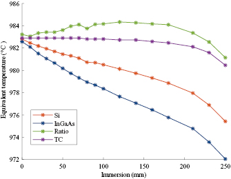
Figure 3. Immersion profiles for the sapphire tube device, with simultaneous recordings of the reference temperature.
Download figure:
Standard image High-resolution imageEach of the bands are highly sensitive to the immersion. There does not seem to be any sign of a saturation behaviour: the trend is linear to the depth of the furnace. In the 200 mm where the thermocouple indicates that the temperature is stable the optically obtained indications drops by approximately 4 °C and 8 °C for the band centered on 0.95 μm and 1.51 μm, respectively.
Also shown is the result of forming the ratio  between the signals. The calibration curve in this case is given by
The constant gain factor K is the ratio between the a1-constants for the  μm and
  μm bands:
  . To simplify notation we have introduced new parameters m2, m3, n2 and n3, which corresponds to the fitted a2 and a3 from equation (2) at 0.95 μm (n) and 1.51 μm (m). The second factor describes the shape of the curve.
The five parameters in equation (4) can be fitted to measurements using  calibration points. A second approach is to fit the Sakuma–Hattori equation for each wavelength, and then construct
  from the fitted constants. This second approach has two attractive features: the minimum number of calibration points is reduced to three, and the fitting of equation (2) is more robust and easier than fitting equation (4). A direct fit of equation (4) requires some search algorithm to identify the minimisation parameters, but the classical least squares minimisation function has several shallow minima that can confuse search algorithms, and leaves the process prone to errors triggered by noise.
Broadly speaking, we now have three different schemes for calibration of the device: (i) a single band centered at 0.95 μm with a narrow response; (ii) a single band at 1.51 μm with a similarly narrow response; and (iii) a ratio formed by dividing the signal at 0.95 μm to the signal at 1.51 μm. The immersion profile suggests that the latter scheme is necessary to avoid an excessive dependence on the use scenario.
4. Calibration uncertainty
The interpolation uncertainty for equation (2), given a set of calibration points  with associated uncertainty, can be evaluated analytically using a procedure described by Saunders [26]. The evaluation follows the principles from the guide to the expression of uncertainty in measurements [27]. Numerical simulations using Monte Carlo modelling (MCM) are a tractable alternative, which with appropriate attention can be used to express coverage intervals in similar ways as in regular analytic evaluation [28, 29]. The numerical evaluation is particularly useful for the ratio model in equation (4), where the uncertainty in the calibration temperatures is correlated in the two wavelengths, because the observations that are used to fit equation (2) are recorded simultaneously. MCM provides a very intuitive way to handle this by simply utilizing the same realisations of temperature for both wavelengths in each iteration. Similarly, the correlation between the photovoltages in each band, which arises because the dark current is evaluated from the same set of observations, is easily handled by using the same realisation of the dark current compensation for all four calibration points.
The evaluation proceeds by drawing pseudo-random numbers used to realise each calibration point  , fit the Sakuma–Hattori equations, and sample the resulting curve at desired points. By repeating the procedure a large number of times one can extract information about the statistical distribution of function values at the sample temperatures.
Table 1 summarises the uncertainty contributions taken into account here. The reference temperature uncertainty budget takes into account calibration of the thermocouple sensor, calibration and resolution of the voltmeter used to read the thermovoltage, and inhomogeneity of the thermocouple wires. It also contains a term to take into account the temperature gradients within the furnace chamber. This term will in general depend on the position in the furnace chamber. The uncertainty estimate stated in the table is based on the measured temperature profile in the stable region, where the gradient is smaller than 2 °C m−1, and scaled with the approximate axial distance between the sapphire tip and the reference sensor (less than 5 mm). We assume that the temperature uniformity in cross sections of the furnace chamber is much better. The uncertainty assigned from the resolution of the voltmeter is scaled with the sensitivity of the thermocouple, and hence depends on temperature.
Table 1. Contributions taken into account for the Monte Carlo computation of calibration uncertainty, where all values stated in the table are standard uncertainties. The same signal contributions are used for the two detectors. In general numeric values differ at each temperature, although with some exceptions. Dark current uncertainty is estimated from the stability and observed noise during its recording.
| Temperature contributions | |||
|---|---|---|---|
| Contribution | Evaluation u | Distribution | Unit |
| Observations | Standard deviation of mean | Normal | °C |
| TC calibration | 0.1 °C | Normal | °C |
| TC inhomogeneity | 0.1 °C | Normal | °C |
| Furnace gradient | 0.01 °C | Normal | °C |
| Resolution |
From voltmeter specifications, scaled with TC sensitivity (typ. 30 mK) | Uniform | °C |
| Signal contributions | |||
| Observations | Standard deviation of mean | Normal | V |
| Dark current | Observed std and stability | Normal | V |
 |
Relative 10−4 | Normal | V |
 |
Relative 10−6 | Normal | V |
 |
Relative 10−6 | Normal | V |
| Resolution | From voltmeter specifications,  |
Uniform | V |
aTemperature dependent. bTemperature coefficients of optical component: BS = beamsplitter, det = detectors, filter = interference filters.
The signal values used in the computations are the dark current compensated voltages from observations. The estimate of the dark current is therefore 0, but the uncertainty is not. The dark current is determined by closing the light path using a shutter inserted just before the beamsplitter (see figure 1). The dark signal is recorded for a couple of minutes before opening the shutter and starting the measurements. The average reading is subtracted from all subsequent measurements. The uncertainty assigned to this correction is Normally distributed with a standard deviation taken from the dark current sequence. In each iteration of the MCM the same realisation is used for all 4 signals from the same detector. The temperature coefficient is assigned a small value here. The data is recorded in a temperature controlled laboratory, and the InGaAs detector is Peltier cooled to reduce the influence of a thermal background. While there may be small changes in temperature during the time of the experiment we expect this to be a small contribution.
Each iteration in the MCM process then draws four values for temperature, four values for corresponding optical signal from the Si detector, a single value for the dark current for the Si detector, four values for the InGaAs optical signals corresponding to the calibration temperatures, and a single value for its dark current. The same realisations of the temperature values are used in both detectors. This procedure ensures that the correlation between the calibrations in the two bands is properly accounted for. The final stage is to fit equation (2) to the 0.95 μm and 1.51 μm observations separately, and the process is repeated 106 times.
The output of the computation is shown in figure 4 for each of the three cases (a single narrow band centered on 0.95 μm, a single narrow band centered on 1.51 μm, and the ratio).

Figure 4. The interpolation uncertainty after calibrating the sapphire tube at four temperatures between 830 °C and 1000 °C. The ratio model always has a higher uncertainty. Beyond the calibration range the uncertainty rises sharply.
Download figure:
Standard image High-resolution image
5. Discussion
For narrow band pyrometry the rule of thumb is that a shorter wavelength provides a smaller uncertainty. There are usually other reasons for selecting long wavelengths, such as signal strength or molecular absorption lines in the medium between the target and the detector. The interpolation uncertainty in our case is similar for the two wavelengths used, which is partly due to the different nature of the detection systems (the voltmeters used, and the detector and preamplifier hardware). It is clear that in terms of a calibration uncertainty, however, either is better than the ratio model.
The observed immersion depth dependence in figure 3 implies that the behaviour of the tungsten filament cannot be adequately described by a simple blackbody radiation model. It is clear that a small calibration uncertainty is not necessarily the optimal criterion for the ultimate performance of the device. In the present case a dual-band ratio detection scheme is more robust to immersion than using a single band detection. A likely explanation for this is the relatively low effective emissivity of the tungsten surface caused by the screening effect of the sapphire tube wall. One of the main attractions of the ratio scheme is that it reduces the influence of emissivity and object size [30]; if the emissivity at the wavelengths  and
and  are
are  and
and  , respectively, the ratio of the thermal signal at the two wavelengths is completely determined by the temperature of the object and the Planck curve:
The prefactor  is constant at all temperatures, and can be determined in a calibration. For this method to work properly in general purpose pyrometry it is necessary to assume (i) that the wavelength dependence of emissivity is the same in calibration and application, and (ii) that the background irradiation is negligible. In our case the former assumption is probably true since we use the same object in calibration and application. The background irradiance is considerable, but its intensity increases with temperature in a way that resembles the radiance from the tungsten. To a first approximation the reflected background increases the radiance from the filament somewhat and just increases the effective emissivities
  and
and  while maintaining the ratio between them. However, if the background irradiation originates from an inhomogeneous temperature background the spectral characteristics of the reflected radiation could change, which clearly has an impact on a dual-band detection scheme. This is a plausible explanation for the observation in figure 3 that, despite the improvements, the ratio scheme also produces a temperature offset compared with the reference thermocouple. The magnitude of the offset remains smaller than the either of the wavelength channels separately. On the other hand, the test case here is a very uniform environment, and ensures that the reflected light behaves in a predictable and consistent way. If powerful background sources are present, such as exposed furnace heating elements, the dual band ratio technique may prove less efficient.
The temperature dependence of the emissivity of tungsten cannot be ignored. It will modify the shape of the light emission with temperature, with the consequence that the Planck law cannot be used uncritically. Using the Sakuma–Hattori approximation can give substantial interpolation errors, larger than the propagated uncertainty in the calibration points. This limits the useful temperature calibration range in any single calibration. To extend the usable temperature range it will be necessary to calibrate the device in subranges and use different calibration curves in each subrange.
The choice of wavelengths for the dual-band detection scheme has not been optimised for a maximum sensitivity [31], but chosen mostly to match the sensitivity of the individual detectors used. The impact of such an optimisation could be pursued elsewhere. Nevertheless, the main observations of a larger calibration uncertainty with the ratio model, but better resilience to changes in the experimental conditions (e.g. immersion), is likely to remain regardless of wavelength choices.
The tungsten filament is also subjected to a non-uniform heat load. The front surface experience a net loss of heat, which is balanced by slightly larger heat gain through the other surfaces. This induces a temperature gradient inside the filament. We have not explored whether this could affect the calibration. However, since the filament is small compared to any reasonable hot zone the device can be used in, we expect the thermal profile inside the filament to be deterministic and very similar in calibration and use scenarios. It is of course conceivable that a strong radiation source could irradiate the front face and modify the temperature gradients inside the filament, but the presence of such a light source would cause other complications, for instance a much stronger reflected signal. The immersion profiles from figure 3 suggests that care is needed if the sapphire tube device is used in highly non-uniform environments.
The in-use uncertainty is dominated by three main contributions: (i) the interpolation uncertainty from calibration, (ii) the interpolation error, primarily due to the temperature evolution of the emissivity, and (iii) the effective immersion depth during usage. Using the narrow calibration range from from 830 °C to 1000 °C the uncertainty is dominated by the immersion behaviour, with expanded uncertainty of 2.1 °C, 3.9 °C and 1.2 °C for the 0.95 μm, 1.51 μm and ratio model, respectively. The figures are computed as the quadrature sum of the three contributions with values taken from the figures 2–4. One crucially important choice is the calibration range. The calculations of the interpolation errors (figure 2) shows that rather than covering a wide range, e.g. from 800 °C to 1500 °C one should strive to use narrower calibration ranges. A practical tradeoff between small interpolation error and an economical number of calibration points might be to use a sequence of adjacent ranges spanning 300 °C–400 °C.
6. Conclusion
We have explored a calibration scheme for a light pipe based temperature probe. The probe consists of a sealed sapphire tube filled with inert gas, with a tungsten filament positioned at the bottom. A number of influences must be taken into account. Because of a strong immersion dependence, probably caused by an impaired optical radiation transfer between the surroundings and the tungsten filament, the optimal scheme requires independent detection of two wavelengths to reduce the sensitivity to background irradiation and temperature induced changes in the filament surface properties.
Acknowledgments
This work was carried out under the 14IND04 EMPRESS project, which has received funding from the EMPIR programme co-financed by the Participating States and from the European Union's Horizon 2020 research and innovation programme. We also thank Aurik Andreu, Jarle Gran and Tim Dunker for helpful discussions.