


Abstract
In this paper, we introduce the use of an infinite-mode double-grating interferometer in investigating the fluid dynamics induced by a thermal lens when an intense laser beam—which we call the pump beam—passes through a liquid sample containing strongly absorbing nanoparticles. As the pump beam passes through the sample in normal conditions, since absorption occurs over the beam's trace, temperature increases and density decreases. The density and temperature changes in the sample can be translated to a phase shift in the passing of a plane probe beam through the sample. By causing two parts of the probe beam to interfere, one part passing from the thermal lens area and the other from another area of the sample spatially separate from the first, it is possible to determine the phase shift value. When the propagation directions of the interfering beams are parallel, infinite-mode double-grating interference fringes are formed. In the infinite mode, the formation and evolution of interference fringes directly reflects any change of density or temperature in the sample. The thermal convection is detected visually and quantitatively determined by chasing the first infinite-mode interference fringe produced. In this work, the measurement of the thermal convection velocity is reported in detail. The measured value is comparable with values obtained with other methods under the same conditions. The proposed method is reliable and very simple; further, the convection process can be visualized in real-time.
Export citation and abstract BibTeX RIS
1. Introduction
In the passing of a laser beam having a Gaussian intensity profile through a medium, such as a liquid, a thermal lens is produced if a part of the beam's power is absorbed. Inspection of the literature reveals that thermal lens formation in liquids and its transient and defocusing properties were reported for the first time by Gordon et al [1]. This effect has been used in measuring thermal and optical properties of materials and the study of a variety of dynamic phenomena. Thermal lensing has been used for the measurement of various characteristics of several different transparent liquid, solid, and gas samples such as the thermo-optical coefficient [2–4], linear and non-linear absorption coefficients [5, 6], non-linear refractive index [7–10], thermal diffusivity [11–13], convection velocity [14–17], pyroelelctric coefficient [18], and thermophoresis [19]. The thermal lensing effect is accompanied by certain other physical phenomena, such as self-phase modulation [20, 21] and dynamic self-diffraction [22, 23]. These effects have been also used in studying the Soret effect [24, 25], monitoring non-radiative relaxation in a medium [26], and so on. A widespread application of the thermal lensing effect is the measurement of very small absorbance, which is called thermal lens spectroscopy [27].
This paper introduces the use of a double-grating interferometer in infinite mode in conjunction with a pump–probe technique, for the investigation of thermal-lens fluid dynamics. By the aid of a dichroic mirror, an intense pump beam and an expanded plane probe beam are aligned along the same direction. These beams pass through a liquid sample consisting of nanoparticles while, directly behind the sample, the pump beam is removed using a suitable bandpass filter and the probe beam is allowed to pass through a double-grating interferometer. The probe beam's wavefront is divided into two parts: one passes through the thermal lens while the other passes through an undisturbed region of the sample. By causing those two parts of the probe beam to interfere, it is possible to determine the phase shift value induced by the thermal lens on the probe wavefront. In the experiments, one of the lateral shearing interference patterns formed by overlapping of the (0,1) and (1,0) diffracted orders of the gratings is recorded using a CCD camera and stored in a computer. The propagation directions of these diffraction orders are parallel, and there is only a lateral shift between them. This situation is brought about by setting a zero value for the angle between the directions of the rulings of the first and second gratings. In this geometry, in the absence of the pump beam, the spatial period of the resulting fringes can be considered as an infinite value; for this reason, we call this method the infinite-mode double-grating interferometer method. When the pump beam turns on, infinite-mode interference fringes appear in the field of view. The evolution of these interference fringes directly reflects any change of density or temperature in the sample. Thermal convection is detected visually and quantitatively determined by chasing the first infinite-mode interference fringe produced. This measurement method is reliable and very simple. In this work, the measurement of the thermal convection velocity for water containing FeOH2 nanoparticles is reported. A maximum convection velocity of  was measured, which is in good agreement with the reported value found with another method under the same conditions [17].
In addition to the measurement of the convection velocity, in this work, the effect of the pump beam's power on the form of the steady-state infinite-mode fringes is experimentally demonstrated. Also, the effect of sample length on the final form of the fringes is visualized. This part of the work shows that the method can be applied to the measurement of other thermal and optical characteristics of the sample. In this work, we address some possible measurements that can be made by utilizing these effects, such as the absorption coefficient, thermal conductivity, non-linear refractive index, temperature profile determination, and so on. However, further considerations are beyond the scope of the current work, and will be published as soon as possible in future works.
It is worth mentioning that a method has been proposed, using a double-grating interferometer (but not in the infinite mode) in conjunction with a pump–probe technique, for measuring the thermal non-linear refractive index of materials [9]. In that work, the refractive index non-linearity was determined by calculating the phases of two interference fringe patterns: the phase profile of the linear interference fringes resulting in the absence of the pump beam and that of the deformed fringes forming in its presence. In that work, the phase maps of the interference fringes were determined by Fourier transform analysis. For the measurement of the non-linear refractive index, this method is simple, stable, and has a high sensitivity. Also, in comparison with the customarily used z-scan method [7], the data acquisition in this method is not a time-consuming process. However, converting the raw data to the desired quantities is still a time-consuming process. As deducing the phase maps of the interference fringes from the recorded data needs a considerable calculation time, it is still not appropriate for use in a real-time study of dynamic phenomena. Therefore, for the real-time investigation of dynamic phenomena, such as the dynamics of a fluid's action in the thermal lensing effect, the use of non-infinite double-grating interferometry is not recommended. In another work, the same setup was used for the measurement of the thermal non-linear optical response of meso-tetraphenylporphyrin under aggregation conditions and determination of the temperature changes induced by the pump beam in the absorbing solution [10].
In this paper, with the aid of infinite-mode fringes and using fringe chasing analysis instead of the phase calculation that was done by the Fourier transform, a real-time method is presented for investigating the dynamics of a fluid acting as a thermal lens. Transition from the previously introduced double-grating interferometer setup to an infinite-mode double-grating interferometer is achieved by merely setting the angle of the gratings' rulings equal to zero. By the mentioned simple change, in the absence of the pump beam the spatial period of the resulting fringes can be considered infinite. But, by passing the pump beam through the sample, infinite-mode interference fringes are made to appear on the field-of-view of the recording plane. The form of the infinite-mode interference fringes visually reflects the forms of the temperature and refractive index changes. One of the nice features of the infinite-mode interferometry method is that it is a direct method that monitors the convection process in real-time. Also, in comparison with the non-infinite-mode double-grating interferometry method, here the phase map calculation for the interference fringe patterns by the Fourier transform method is removed from the process. This setup is still simple, stable, and has a high sensitivity.
In the following two sections, the infinite-mode double-grating interferometry is described, and a brief formulation for the resulting infinite-mode fringes presented, respectively.
2. Infinite-mode double-grating interferometry
A schematic diagram of the experimental setup is shown in figure 1. The probe beam, which is an expanded monochromatic plane beam, passes through two identical gratings, G1 and G2. The separation of the gratings is denoted by L, and the angle between the directions of the rulings of the first and second gratings is zero. The incident plane probe wave before G1 will be distorted in the area in which the pump beam propagates through the sample—see figure 2. The two laterally displaced interfering beams are the result of two subsequent positive first-order and zero-order diffractions by the two gratings, and vice versa: one beam through the sequence zero-order → positive first-order, u(0,1), the other through the sequence positive first-order → zero-order, u(1,0). Thus, the interfering beams are mutually parallel after passing through the two gratings. By the aid of a diaphragm, behind the interferometer, all other diffraction combinations are intercepted. A lateral shear, with a value larger than the size of the distorted area on the probe wavefront, is chosen between the two interfering diffraction orders. Also, the distance between G2 and the recording plane should be larger than  , where λ is the wavelength of the probe beam, p is the grating period and D is the diameter of the probe beam at the gratings. This condition guarantees that no other diffraction orders overlaps with the desired interference pattern. In fact, the distorted interference pattern consists of the superposition of the two laterally displaced interfering wavefronts: the unchanged plane wavefront and the affected carrier wavefront.
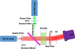
Figure 1. Schismatic diagram of the measurement setup, G1 and G2 are two identical gratings.
Download figure:
Standard image High-resolution image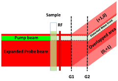
Figure 2. Illustration of two-grating interferometry in the infinite mode. Propagation directions of the interfering diffracted orders (0,1) and (1,0) are parallel.
Download figure:
Standard image High-resolution image3. The phase shift induced in the sample has the same form of the phase of the resulting interference fringes
When the pump beam is off, both of the amplitudes of the interfering orders of the probe beam can be considered as plane beams:

where A is the amplitude,  is the propagation vector of the waves (
 ), and λ is the probe beam wavelength. In this case, over the interference pattern, for an ideal case of the plane probe beam, the intensity has the constant form of
  ; consequently, the phase also has a constant value over the interfering area and can be considered equal to zero:
  .
.
As the pump turns on, its optical field induces refractive index changes in the sample. Any changes in the refractive index of the medium can be translated to a phase-shift on the probe beam. It is considered that at t = 0 the pump beam turns on or is allowed to pass through the sample. In this case, the interfering fields can be written as
where  is the phase shift induced by the pump beam in the medium at a time t, and can be calculated as
where  is the refractive index of the sample in the absence of the pump beam, z is the propagation direction, and d is the length of the sample. Because the lateral shear is larger than the diameter of the pump beam, it is assumed that u(1,0)(x,y) is not affected by the pump beam in the selected area of the interference pattern—see figure 2. Now, the interference pattern is given by
In this case, the resulting infinite-mode interference pattern has the following phase distribution:

Therefore, the distribution of the phase shift induced on the probe beam due to the interaction of the pump beam with the matter, is the same as the phase map of the resulting infinite-mode interference fringes. In other words, the formation and evolution of the interference fringes directly reflect any change of density or temperature in the sample.
For small values of t, when the convection effect can be ignored, due to the Gaussian intensity profile of the pump beam, the phase modulation,  , has a Gaussian profile, too.
When the size of the fringes remains unchanged in the horizontal direction, and at the same time the upper parts of the resulting fringes are stretched toward higher altitudes, it can be concluded that convection is the dominant effect. In this case, in fact, a local change in the temperature, density, and refractive index moves upward with the bulk movement due to the convection flow, and—as a result—the fringe pattern gradually acquires an asymmetric form. The maximum value of the bulk movement can be estimated by measuring the asymmetry of the resulting fringes, where buoyancy occurs. The formation of asymmetric fringes due to the presence of convection flow can be predicted via appropriate mathematical formulation. This theoretical work is under study.
3.1. Pump beam absorption induces refractive index changes in the sample
The complex amplitude of the pump beam at the input plane of the sample, z = 0, can be written as
where  is the on-axis amplitude of the beam, P is the total power of the beam, w is the radius of the beam (HW1/e2M, say), k is the wavenumber, and R is the beam wavefront radius.
The intensity of the pump beam after propagating the z distance through the medium with an absorption coefficient of α can be written as
The heat generated by the pump beam per unit time and unit volume of the sample at position  is given by

The refractive index changes can be given by
where  is the thermo-optical coefficient of the medium and
  is the temperature distribution induced by the absorbed pump beam energy. Since the intensity profile of the pump beam is Gaussian, for small values of t that guarantee convectionless conditions, any temperature and resulting refractive index changes within the sample will also follow a similar profile. t is measured from the turning on of the pump beam. The temperature distribution induced by the absorbed pump beam energy,
  , can be determined by using the Green's function for the heat conduction and convection equation [21]. Finally, the desired phase shift profile translated on the probe beam is determined as function of t by the following relation [21]:
where  is the characteristic heat diffusion time,
  is the thermal diffusivity of the sample, K is the thermal conductivity, ρ is the density, cP is the specific heat of the sample, and
  is the on-axis phase shift.
As is apparent from equation (10), the value of phase shift induced in the sample is related to the thermal and fluid dynamics parameters. These parameters and some other setup and sample parameters, such as the pump beam path depth from the free surface of the sample and dynamic viscosity coefficient of the sample, affect the measured value of the convection velocity. In the current work, the value of the convection velocity is measured for the given values of the sample and setup parameters. Investigating the dependency of the convection velocity on each of the thermal and fluid dynamics parameters of the sample and the setup parameters is a very interesting and relevant issue. This work is under study.
4. Experimental setup and parameters
The infinite-mode double-grating interferometer setup used to measure the convection velocity is shown in figure 1. A 5 mW He–Ne laser beam with a wavelength of 632.8 nm is expanded and collimated. We have utilized the technique for measuring the convection velocity of a water solution containing FeOOH nanoparticles. In the measuring convection velocity of the water solution, two Ronchi gratings G1 and G2, with the same pitch p = 10 μm and a separation of 4 cm were used. In this measurement, the volume percentage ( ) of FeOOH in the solution was 0.8%, their sizes were about 5 nm, and cell thickness was 2 mm. The pump beam's path was about 17 mm under the free surface of the water, and the pump beam's wavelength and its radius inside the sample were 532 nm and 0.5 mm respectively. The power of the pump beam at the sample was 40.2 mW. The second harmonic of a 50 mW continuous wave (CW) diode-pumped Nd:YAG laser beam at 532 nm was used as the pump beam. The desired power was prepared on the sample with the aid of a neutral density filter. The setup with the mentioned specifications of the system was used for the convection velocity measurement that is presented in section 7.
As, for the various experiments, some of the setup and sample parameters were modified, all the necessary parameters of the setup and sample of the experiments are presented in table 1.
Table 1. Sample and solution, and varying parameters of the setup used in the various measurements.
| Figure no. (varying parameter) | Sample, solution (conc. or %V/V) | Power of pump (±0.01) (mW) | Cell thickness (mm) | Gratings apart (±0.1) (cm) | Depth of pump beam path (±1) (mm) |
|---|---|---|---|---|---|
| Figures 3, 8 and 9 (time) | Water, FeOOH (0.8%) | 40.2 | 2 | 4 | 17 |
| Figure 4 (power) | Thinner, Fe3O4 (3 mM) | 0–30 | 2 | 3.5 | — |
| Figure 6 (time) | Thinner, Fe3O4 (3 mM) | 30 | 7 | 3.5 | — |
| Figure 7 (time) | Thinner, Fe3O4 (3 mM) | 30 | 7 | 3.5 | — |
| Figure 10(a) (time) | Thinner, Fe3O4 (0.005%) | 5 | 5 | 7 | 15 |
| Figure 10(b) (time) | Thinner, Fe3O4 (0.005%) | 12.73 | 5 | 7 | 15 |
| Figure 11 (time) | Thinner, Fe3O4 (0.005%) | 38.6 | 5 | 7 | 15 |
5. Formation and evolution of the interference pattern
In figure 3, formation and evolution of the experimentally recorded infinite-mode interference pattern at various times after propagating a CW pump beam through a water solution containing FeOOH nanoparticles are shown. The pump beam's power at the sample was 40.2 mW.

Figure 3. Formation and evolution of an interference pattern in an infinite-mode two-grating interferometer immediately after propagating a CW pump beam through a water solution containing FeOOH nanoparticles with particle size 5 nm and a volume percentage of 0.8%. Cell length was 2 mm, the pump beam's path was about 17 mm under the surface of the water, gratings' periods were 10 μm and their separation 4 cm, the pump and probe beams' wavelengths were 532 nm and 632.8 nm respectively, and the pump beam's radius inside the sample was 0.5 mm. All sizes are in millimeters. The blue circles and green triangles on the patterns show displacement of the first introduced dark fringe at various times in the vertical and horizontal directions, respectively.
Download figure:
Standard image High-resolution imageSome of the most significant observations follow:
- 1After passing the pump beam through the sample, three different time intervals based on the form of the resulting fringes are distinguished.
- 2From the time the pump beam is switched on—say, time 0—till a specific time t1, we have symmetric concentric circular fringes. These symmetric fringes are formed over the path of the pump beam. In this time interval, by increasing the time, the number of the resulting fringes increases—see figures 3(a) and (d).
- 3After time t1, the fringes become asymmetric due to convection flow, and continue to evolve till another specific time t2, in which we suppose this evolution reaches a steady state. In the presence of the convection flow, the resulting infinite-mode fringes are distorted on the top side, and this behavior continues to develop until t2—see figures 3(e)–(i). In these patterns, an upward shift for the maximum values of the phase shift also appears. The observed value for the time interval of
 is of the order of seconds.
 - 4The third time interval begins after time t2, when the fringes reach a steady-state form.
- 5We also observed that, on turning off the pump beam or interrupting the beam, it required a time comparable with that of the 'turn-on' transient, t2, for the liquid to recover.

For a given measurement, the specific times t1 and t2 are related to the thermo-optical characteristics of the sample, such as absorption coefficient, diffusivity, and thermal conductivity, the specifications of the measuring system, such as the pump beam's power, and the geometric parameters of the setup, such as the depth of the pump beam's path from the sample surface.
It is worth mentioning that, in some specific cases, such as the case of very high value absorption coefficient of the sample and high power pump beam, at large values of t, instead of the steady-state form, the resulting fringes experience periodic changes by the time. This effect has a heartbeat-like appearance and is related to the formation and flotation of successive bubble-like bulks produced in the sample. This phenomenon is know as thermal lens oscillation, and has previously been investigated by other methods [28–30]. For certain liquids, such as ferrofluids, we observed this optical heartbeat phenomenon. Study of this effect by the aid of infinite-mode interference fringes has some advantages, but is beyond the scope of the current work.
6. Steady-state infinite-mode interference fringes
Here, some experimental results are presented that show the completely developed forms of the resulting fringes at different conditions. We call these patterns steady-state infinite-mode fringes. We show, via the experimentally recorded patterns, the effects of various pump beam powers and sample lengths on the final form of the steady-state infinite-mode fringes. Further considerations in this regard are left to future works.
6.1. Effect of pump beam power on the steady-state infinite-mode fringes
In figure 4, we demonstrate a set of infinite-mode fringes experimentally recorded at the steady state when pump beams of various power are applied. These results correspond to the measurements which were performed on 3 mM concentration of Fe3O4 nanoparticles in oil thinner solution, in a 2 mm thickness cell; the gratings' periods were 5 μm and their separation 3.5 cm, the pump and probe beams' wavelengths were 532 nm and 632 nm, respectively, and the pump beam's radius inside the sample was 0.5 mm. In this figure, from (a) to (p), power values of the pump beam are changed in equal steps between zero and 30 mW. All patterns were recorded 30 s after the passing of the pump beam through the sample.
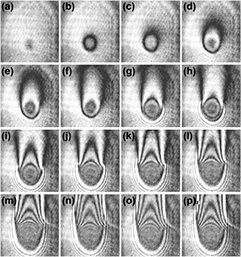
Figure 4. Steady-state infinite-mode interference patterns obtained with various values of pump beam power. For all patterns, the sample was a solution of oil thinner containing Fe3O4 nanoparticles with a concentration of 3 mM, cell thickness was 2 mm, grating periods were 5 μm and their separation 3.5 cm, pump and probe beam wavelengths were 532 nm and 632 nm respectively, and pump beam radius inside the sample was 0.5 mm. From (a) to (p), the pump power was changed with equal steps between zero and 30 mW. All patterns were recorded after 30 s from turning on the pump beam.
Download figure:
Standard image High-resolution imageAs is apparent, for the low power cases shown in figures 4(a) and (b), the resulting fringes have symmetric forms, meaning there is no convection flow in the sample. For these values of pump power, the transient behavior does not appear. On increasing the pump beam's power, as shown in figures 4(c)–(p), the number of the resulting fringes increases over the field of view.
In figure 5, a typical steady-state infinite-mode fringe pattern is shown. As is apparent, a recorded fringe pattern can be divided into three distinct areas; patterns over areas A and B are interference fringes, but the pattern observed over area C is a result of diffraction by the induced thermal lens, called diffraction fringes. Creation of a thermal lens in the sample causes an abrupt phase change on the probe beam over the lower boundary of thermal lens where there is no convection flow.

Figure 5. Dividing a recoded pattern into three distinct areas.
Download figure:
Standard image High-resolution imageThe central area shown by the letter A corresponds to the path of the pump beam through the sample. As shown in figures 4(j)–(l), on increasing the pump beam power, the visibility of the resulting fringes decreases, such that for figures 4(m)–(p), the fringe patterns on area A disappear.
The resulting recorded fringes in area A are interference fringes, and are observable for the cases in which the power of the pump beam is low. They have a radial symmetry. On increasing the pump beam's power, the number of the resulting fringes in this area increases. For larger values of pump beam power, these fringes disappear. We guess that this effect might be originated by one or both of the following physical reasons: due to the creation of a turbulent flow in that area that wipes out the interference fringes, or due to increase of the limited spatial resolution of the recording system.
Fringes over the transient area indicated by B in figure 5 are affected by the convection flow in the sample. The resulting fringes over the area determined by C in figure 5 are diffraction patterns of the probe beam from the thermal lens phase object. As the thermal lens is a phase object, the probe beam is diffracted by its bottom side boundary due to the abrupt phase shift there [31]. As over the top side of the thermal lens area the refractive index changes gradually, there is no diffraction effect on this side. The diffraction pattern in area C was also used for characterization of the thermal lens [20, 21]. The use of diffractometry in thermal lens studies is time-consuming, and is an indirect method.
6.2. Sample length effect on the infinite-mode fringes
In figure 6 effects of sample length on the form of the resulting fringes are shown. As is apparent, an increase in the sample length causes an increase in the number of resulting fringes, especially in area A, without any decrease in visibility. This figure shows the method's capability in the measurement of other thermal and optical characteristics of the sample. These results directly address to some possible measurements, such as the absorption coefficient, thermal conductivity, non-linear refractive index, temperature profile determination, and so on. However, further considerations are beyond the scope of the current work.

Figure 6. Effect of the sample length on the resulting patterns during transient process. All parameters are the same as in the case of figure 4 except here the cell thickness was 7 mm and power for the pump beam was 30 mW.
Download figure:
Standard image High-resolution image6.3. Liquid recovery time after turns off the pump beam
The discussion in this section is focused on the observation numbered 5 which is given in section 5. The liquid recovery or equally its reverse transient behavior can be easily visualized by interrupting the pump beam after formation of a steady-state infinite-mode fringes. In figure 7, the backward evolution of the resulting fringes immediately after removal of the pump beam are shown. It can be visually estimated that when the pump laser was turned off by interrupting the pump beam, it required a time comparable with that of the 'turn-on' transient for the liquid to recover.
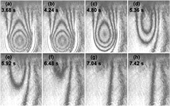
Figure 7. Evolution of the resulting pattern immediately after removing pump beam. All parameters are same as the case of figure 6 except here the pump beam was turned off at t = 3.68 s.
Download figure:
Standard image High-resolution image7. Measuring the convection velocity by chasing infinite-mode fringes of the transient state
Here, measurement of thermal convection velocity in a water sample containing FeOOH nanoparticles is presented. For this propose, the data illustrated in figure 3 is used. As is apparent, the thermal convection can be quantitatively determined by chasing the first infinite-mode dark interference fringe produced. We refer to the locations of the blue circles and green triangles plotted in figure 8. These circles and triangles show the displacement of the first dark fringe introduced at various times in the vertical and horizontal directions, respectively.

Figure 8. Measured displacements in the vertical and horizontal directions for an initially detected temperature wavefront by chasing the first produced dark fring of figure 3.
Download figure:
Standard image High-resolution imageAs is shown in figure 8, displacements of the first dark fringe in the vertical and horizontal directions are equal until almost t = 1 s. In this time interval, absorption occurs and thermal lens formation is completed. After that time, convection flow appears, and as a result the first dark fringe is displaced away in the vertical direction, but in the horizontal direction it comes back slightly. This effect can be explained by the Soret effect.
It is a simple task to calculate velocity of the first dark fringe in the vertical and horizontal directions. In figure 9, the calculated velocities of the initially detected temperature wavefront in the vertical and horizontal directions are plotted. The calculated velocity in the vertical direction is considered as the convection velocity.

Figure 9. Measured velocities along vertical and horizontal directions for an initially detected temperature wavefront.
Download figure:
Standard image High-resolution imageAs is shown in figure 9, the maximum value of the convection velocity in the vertical direction is 0.95 mm/s, and its mean value is approximated by  .
.
It is worth mentioning that the first fringe displacement was determined in the vertical direction as a function of time by chasing the location of the extremum value of intensity over the fringe width on successive frames. As in the experiments, the resulting interference fringes were imaged directly onto the sensitive area of a camera without any magnification, and the pixel size of the camera in both directions is 5.2 μm; this value of the pixel size can be considered as the accuracy of the fringe location determination. It is possible to increase the precision of the fringe chasing by using sub-pixel accuracy for the measurement of fringe displacement [32].
As is apparent from figure 9, for the horizontal direction after t = 2 s the velocity of the first dark fringe is negative, which is due to the change of the concentration of the nanoparticles in the temperature gradient where there is no gravitational effect in that direction.
The observed 'quasi-oscillatory' behavior over the time interval 1.5–5 s for the calculated velocity in the vertical direction, the convection velocity, might be related to the previously introduced thermal lens heartbeat effect.
We show that the convection process is visualized in real-time. Also, this measurement is reliable and very simple.
To show the repeatability of the experiments, here results of two sets of measurements are presented. In each set, a measurement was repeated several times without changing the setup and sample parameters. The results of three repeats of an experiment are presented in figure 10(a), and in figure 10(b), the results of four repeats of another experiment. For both sets of experiments, a sample of Fe3O4 nanoparticles in thinner solution with a volume percentage of 0.005% was used; cell thickness and depth of the pump beam path from the free surface were 5 mm and 15 mm respectively. The values of the pump beam power in figures 10(a) and (b) were 5 mW and 12.73 mW respectively. From plots (a) and (b) of figure 10, it can be concluded that the convection velocity is strongly affected by the value of the pump beam power.
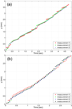
Figure 10. Illustration of repeatability of the fringe chasing method. Measured displacements of an initially detected temperature wavefront in the vertical direction as a function of time with a pump beam power of (a) 5 mW and (b) 12.73 mW. All other sample and setup parameters are the same, and are presented in table 1.
Download figure:
Standard image High-resolution imageNow, the measurement results are validated using particle image velocimetry (PIV) [33–35]. In this method, some small particles are added to the sample in which in the absence of convection velocity, the particles almost behave as suspended objects. In the presence of convection velocity, the motion of particles in the sample is traced by an imaging system. In contrast to the fringe chasing method, we call this method the particle imaging method. In the experiment, the convection motion was made visible by adding some commercial baby powder (ingredients: Hydrated Magnesium Silicate, Perfume) to the sample, and the average velocity of groups of powder particles in thermal lensing area was determined by particle image velocimetry. The average diameter of the particles was around 30 μm. When the pump beam was off, we observed that particles of larger diameter slowly settled, but a significant portion of the powder particles were suspended. When the pump beam was on, successive images of the convection area were recorded by a digital camera, and the convection velocity estimated by tracing the motion of the groups of powder particles.
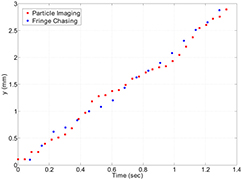
The convection velocity were measured in the same sample when the pump beam was on, for both particle image velocimetry and the fringe chasing method. The measured data for both methods are presented in figure 11. As is apparent, the measured values of the two methods are compatible. In these measurements, a large value of the pump beam power—38.6 mW—was used, to provide a large value of convection velocity and thus to increase the reliability of the particle image velocimetry.
Figure 11. Measured fringe chasing and particle imaging displacement values in the vertical direction for the same sample and setup parameters. All of the parameters are presented in table 1.
Download figure:
Standard image High-resolution image
It should be mentioned that the particle image velocimetry method itself suffers from several serious sources of error—for more details see [35]. The main error arises from the acceleration of the particle in the sample, when the suspension condition does not occur in the off time of the pump beam. Another important point that should be emphasized here is that only during the time of interference fringe development, say during the time interval  introduced in section 5, can we use this kind of comparison of results between the fringe chasing and particle imaging methods. In fact, at the time t2, the distributions of temperature and density in the sample reach stable profiles, as a result of which the interference fringes gain a stable form and the convection flow reaches a steady state. The steady state convection flow guarantees transfer of the heat from the thermal source (or thermal lens area) to the upper area in the sample. Therefore, the fringe chasing method can only make the transient convection velocity measurable; but the particle image velocimetry can be used for the estimation of the steady state convection velocity even for a time bigger than t2. Further consideration in this regard is beyond the scope of the current work.
8. Conclusion
This work introduces the use of a double-grating interferometer in infinite mode in the investigation of the fluid dynamics induced by a thermal lens in the presence of nanoparticles in a pump–probe scenario. The thermal convection was visually detected and quantitatively determined by chasing interference fringes. The repeatability of the presented method was experimentally verified. The measurement results were also validated by comparison with the results obtained by particle image velocimetry; the experiment showed that the measured values are comparable. In addition, in this work, the effect of pump beam power on the form of the steady-state infinite-mode fringes was experimentally demonstrated. Also, the effect of sample length on the transient form of the fringes was visualized. This part of the work shows that the method can be applied to the measurement of other thermal and optical characteristics of the sample.
Acknowledgments
The authors thank the anonymous referees for their constructive comments. Also, S.R. acknowledges support from the IASBS Research Council under Grants No. G2015IASBS12632.