
Abstract
Hyperuniformity is evolving to become a unifying concept that can help classify and characterize equilibrium and nonequilibrium states of matter. Therefore, understanding the extent of hyperuniformity in dissipative systems is critical. Here, we study the dynamic evolution of hyperuniformity in a driven dissipative colloidal system. We experimentally show and numerically verify that the hyperuniformity of a colloidal crystal is robust against various lattice imperfections and environmental perturbations. This robustness even manifests during crystal disassembly as the system switches between strong (class I), logarithmic (class II), weak (class III), and non-hyperuniform states. To aid analyses, we developed a comprehensive computational toolbox, enabling real-time characterization of hyperuniformity in real- and reciprocal-spaces together with the evolution of several order metric features, and measurements showing the effect of external perturbations on the spatiotemporal distribution of the particles. Our findings provide a new framework to understand the basic principles that drive a dissipative system to a hyperuniform state.
Export citation and abstract BibTeX RIS

Original content from this work may be used under the terms of the Creative Commons Attribution 4.0 licence. Any further distribution of this work must maintain attribution to the author(s) and the title of the work, journal citation and DOI.
1. Introduction
Hyperuniformity has emerged as a powerful concept that provides a metric to characterize and quantify the orderliness of a given system [1, 2]. One of its seminal findings is the anomalous suppression of density fluctuations at infinite wavelengths for certain statistically isotropic systems, similar to perfect crystals albeit without Bragg peaks [1, 2]. This finding led to rapidly growing research efforts on the investigation of hyperuniformity in different physical systems [3–14], the controlled formation of hyperuniform structures [15–17], and fabrication of lasers, optical and photonic devices using hyperuniform materials [18–23].
A large body of work studied the hyperuniformity of equilibrium systems in the past two decades. A comprehensive review can be found in reference [2]. In contrast, studies on nonequilibrium systems started merely a few years ago to address a basic question: what are the dynamics that drive a dissipative system to a hyperuniform state? This open question stirred much interest to study hyperuniformity in several experimental and theoretical model systems ranging from glass forming and jammed systems [6, 7, 24–27] to driven and diffusive ones [28–34], systems with active particles and fluid states [35–38], self-organizing systems and many more [2, 39, 40].
The majority of these studies associated the emergence, evolution, or disappearance of hyperuniformity to a similar set of dynamics common to different model systems. These dynamics include but are not limited to the presence of diverse sources of noise, fluctuations, imperfections, perturbations, external fields, and many-body interactions [2, 6, 7, 24–40]. Discovering such commonalities is significant and further strengthen the idea of hyperuniformity becoming a unifying concept. However, such unification of many physically different systems under the hyperuniformity concept calls for a general theoretical framework, which is still in its infancy [2]. Further research on new model systems with distinct internal dynamics will surely accelerate its development.
Here, we show the dynamic evolution of hyperuniformity in a unique driven dissipative model system [41–44] during the disassembly of a colloidal crystal. We experimentally show and numerically verify that the system switches between strong (class I), logarithmic (class II), weak (class III), and non-hyperuniform states. Importantly, we show that the hyperuniformity is preserved even long after the external energy input has been removed from the system. We postulate that the internal feedback mechanisms present in our driven dissipative system are responsible for the long-lived hyperuniformity despite varying degrees of lattice imperfections, noise, fluctuations, random vectorial fluid flows, and structural inhomogeneities that continuously perturb the system. We further present real-time analysis of all these effects on our system's hyperuniformity via a unique computational toolbox.
2. Experiments and the computational toolbox
2.1. Experiments
The experimental system is the same as in references [41, 42], where detailed explanations are provided on the setup and its operational dynamics. As can be seen from figure 1(a), the setup consists of a femtosecond laser (Spectra-Physics, Spirit One 1040-8-SHG, 1040 nm wavelength, 1 MHz pulse repetition frequency, and ∼6 μm spot size) coupled to an inverted microscope (Nikon, Eclipse Ti-U). The experiments are performed on a quasi-2D-confined, monodispersed pure polystyrene spheres (1 μm in diameter) suspended in water (2 wt%, microparticles GmbH). Experiments are recorded using a CMOS camera (DCC1645C-HQ, Thorlabs) with 1280 × 1024 pixels and a rate of 15 frames per second. A blue LED is used for imaging illumination.
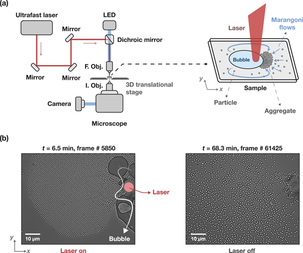
Figure 1. (a) A representative schematic of the experimental setup. The extended schematic on the right shows the formation of a cavitation bubble and the Marangoni flows when the laser is on. Dragged particles are shown to self-assemble at the bubble boundary. (b) Microscope images show self-assembled hexagonal crystal formed at the bubble boundary when the laser is on (left), disassembled when the laser is off (right). The images denote the start and the end frames of the analyses presented in this study.
Download figure:
Standard image High-resolution imageAs detailed in references [41, 42], initially, the system has a statistically isotropic distribution of Brownian particles. Upon turning on the laser, a cavitation bubble forms along with laser-induced Marangoni flows, which drag the particles towards their aggregation at the bubble boundary (figure 1(b), left). Turning off the laser stops the drag flow, and particles disassemble back into the system, eventually relaxing to an isotropic distribution (figure 1(b), right).
Thirty experiments have been performed for this study. Although we confirmed our central claims for all experimental video recordings, combining these experiments to provide ensemble averaging of specific quantities such as number variance was not possible because each experiment is necessarily different as neither the sequence nor the exact location of lattice imperfections or external perturbations can be repeated in this strongly stochastic system. Nonetheless, the evolution of hyperuniformity from class I to class II, class III, and non-hyperuniform states was observed and quantified for each experiment. Due to the sheer amount of data, we cannot provide the results of all experiments here. Therefore, we present our analyses over one experimental video, which can be viewed from video 1 (https://stacks.iop.org/JPCM/33/304002/mmedia). We further offer appendix figure 11 and appendix table 3 that show the same analysis as in figure 3 performed on a different experiment.
Video 1 is divided into four parts since camera recording stops automatically upon hitting the file size limit of 4 GB. The original recording of ∼1 h is sped up 15 times to reduce the duration to roughly 4 min. The experimentalist immediately starts recording a new video with roughly 20 s of data acquisition gaps between each part.
The first part of the video shows the formation of a nearly perfect hexagonal crystal at a cavitation bubble boundary. The red square frame in the video (orange square frame in figure 2(b)) indicates the field of view (720 × 720 pixels) where we perform our analyses. The analyses start at t = 6.5 min (frame # 5850) (figure 1(b), left), and end at t = 68.3 min (frame # 61425) (figure 1(b), right). The laser position is denoted in figure 1(b), left.
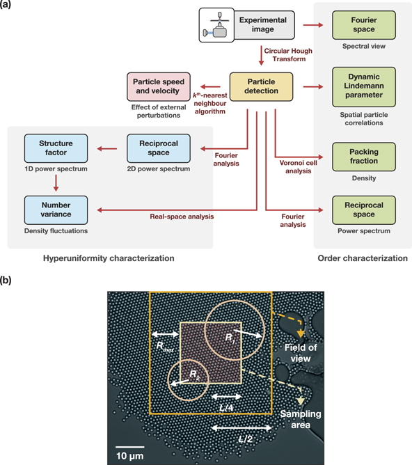
Figure 2. (a) A logic map of the computational toolbox developed for real-time analyses. (b) The size and position of the field of view and sampling area are marked on a microscope image. The red dots within the sampling area represents the centres of the circular observation windows with different radii.
Download figure:
Standard image High-resolution imageAs can be seen from the video, the system is highly dynamic. Particles never stop their motion even when they are embedded into the crystal. In part 2, the experimentalist turns off the laser, and the crystal disassembles. As will be discussed in section 3, during this disassembly, various lattice imperfections such as line and point defects, dislocations, and voids emerge, propagate, and annihilate because physical boundaries change (e.g., bubbles shrink and vanish), additional vectorial fluid flows emerge, and the particles' motions increase. All these changes are reflected in the spatiotemporal distribution of the particles and the interparticle correlations.
Upon turning off the laser, crystal disassembly starts from the lower corners of the field of view (figure 4(b)) resulting an inhomogeneous spatial and velocity distribution of particles. Particles at the lower corners move faster than those in the middle and at the upper corners. Roughly at around t = 18 min (frame # 16229), half of the field of view is solid-like and the other half is liquid-like (figure 4(c)). Our analyses continue in parts 3 and 4 of video 1 until t = 68.3 min (frame # 61425).
2.2. The computational toolbox
The system has relatively fast dynamics, and to assess their effect on hyperuniformity we developed a computational toolbox to perform real-time analysis on video 1. This toolbox provides the simultaneous characterization of hyperuniformity in real- and reciprocal-spaces together with the evolution of several different order metrics and measurements showing the effect of external perturbations on particle movements. On-the-fly analyses of the experiments can be viewed from video 2, a logic map to these analyses is given in figure 2(a), and appendix figure 12 shows a representative screen view of the toolbox.
2.2.1. Particle detection
We start all our analyses with particle detection using an algorithm based on circular Hough transform (CHT) [41, 42]. The first step is to enhance the contrast of the input images (i.e., video frames) by adjusting their grayscale level to be between two threshold values, namely, the brightness of the particles (high-level threshold) and that of the background (low-level threshold). This way, the dynamic range of the input images is increased, and background noise is filtered out. The next step is to apply a morphological dilation operator with a disk-shaped (also called the rolling ball) structuring element that enhances particles' circular shape and enlarges them to increase the detection accuracy. The final step is to apply CHT in Matlab using the native command 'imfindcircles' to generate the detected particles' centre coordinates. Appendix figure 13 shows the results of these detection steps for three arbitrarily chosen video frames.
We optimize the CHT parameters to increase the detection accuracy, namely, we adjust the search range radius of the circles, detection sensitivity, and edge threshold. To set optimal values of these parameters for full frame-span, the detection accuracy is verified initially by running it over a number of randomly selected frames. Then accurate detection is confirmed with the output analysis video that is generated for each input video. These parameters need to be optimized only once for any set of experimental video recordings that share similar imaging conditions (i.e., particle size, imaging objective, and illumination conditions).
After the particle detection step, we perform an analysis of Fourier- and reciprocal-space, dynamic Lindemann parameter, and packing fraction to characterize the system's orderliness. The effect of external perturbations on the spatiotemporal distribution of the particles are monitored through particle speed and velocity maps. The system's hyperuniformity is analysed using local and scaled number variance curves and the static structure factor calculations. Furthermore, we show two alternative number-variance calculations, namely, sampling of the real-space using circular observation windows with varying radii (figure 2(b)), and directly from the power spectrum.
Video 2 screen is divided into 3 by 3 windows (appendix figure 12). The first window at the top row shows frame-by-frame experimental images within the designated field of view shown in video 1 and figure 2(b). Time and frame numbers written at the top of this window match those in video 1.
2.2.2. Dynamic Lindemann parameter map
The second window at the top row of video 2 and appendix figure 12 is the dynamic Lindemann parameter  [41, 45, 46], which gives a local measure for interparticle distances through
where  is the average distance between particles, i, and its neighbouring particles. The averages can be calculated by
  , where
  is the total number of particles in the scan area of the particle i (i.e., the circular region with a radius of 2.8 times the particle radius surrounding the particle i), including the particle i itself. j is an integer index scanning over all neighbouring particles.
Values of the dynamic Lindemann parameter per particle lie between 0 and 1, which are also colour-coded. Particles that are distant and independent of each other, similar to the gaseous state, are coloured red,  . Particles are coloured blue if their neighbouring particles are at their close-packing arrangements,
  , as in the solid-state. Particles coloured in between are neither distant and independent of each other, nor they are close-packed,
  , similar to the liquid state or, e.g., particles at the grain boundaries [41]. The colour map of the dynamic Lindemann parameter gives a visualization of the particles' spatial correlations and clearly shows the position and propagation of various lattice imperfections frame-by-frame.
2.2.3. Packing fraction
The last window at the top row of video 2 and appendix figure 12 is the packing fraction, ϕ, which is calculated through Voronoi cell analysis using [47, 48]

where Ntotal is the total number of particles, D is the average particle diameter, and A is the aggregate area calculated using the Voronoi diagram. The calculation of A is performed using Matlab function 'voronoin', then adding up the areas of the inner Voronoi polygons. A plot showing time evolution of the packing fraction can be seen in appendix figure 14.
2.2.4. Particle speed and velocity maps
Our first step was to optimize the detection and tracking accuracy by analysing the experimental videos recorded with different frame rates. We then chose a sufficiently high frame rate such that no particle can move more than its radius between two consecutive frames.
The first two windows at the second row of video 2 and appendix figure 12 show the particle speed and velocity maps, which strikingly visualize the effect of environmental perturbations on their spatiotemporal distribution. As detailed in section 2.2.1, we first detect each particle frame-by-frame, which gives us their positional x- and y-coordinates. The coordinates are then fed to a nearest neighbour search algorithm to trace the particles and compute their speed and velocities. For each particle in a given frame, we find the closest neighbouring particle in the previous frame and calculate the displacement of their centres via Matlab's kth-nearest neighbour search algorithm for k = 1.
We exclude the particles near the edges within a margin equal to the particle diameter to avoid particle detection and tracking errors near the edges of the field of view. Particle velocities are computed by multiplying their displacements by the frame rate.
Similar to the dynamic Lindemann parameter map, the speed map is also colour-coded between blue and red to visualize the slowest (blue) and fastest (red) moving particles.
2.2.5. Fourier and reciprocal space images
The last window at the second row of video 2 and appendix figure 12 shows Fourier- and reciprocal-space images to visually assess the system's structural symmetry frame-by-frame. The Fourier image is the absolute value of 2D fast-Fourier-transform (FFT) of the real image. The reciprocal-space image is calculated using FFT on the point distribution, corresponding to detected particle positions in the real image.
2.2.6. Hyperuniformity characterization
The last row of video 2 and appendix figure 12 shows hyperuniformity characterization through local and scaled number variances and static structure factor calculations.
We used monodispersed hard-sphere particles with identical diameters (1 μm on average). Naturally, the system can be treated as a point configuration, and hyperuniformity can be assessed from the number variance [2, 6]. However, we additionally calculate the volume fraction variance since our system comprises colloidal particles suspended in water and can be regarded as a two-phase system. The volume fraction variance analyses are provided in the appendix figure 15, which do not contradict our claims on hyperuniformity based on the number variance analyses.
We calculate the number variance from both real-space and reciprocal-space (i.e., the power spectrum). The two methods are performed simultaneously over the same field of view with a fixed size (720 × 720 pixels) and position throughout the experimental video.
For real-space analysis, we choose half of the field of view (360 × 360 pixels) as the sampling region (figure 2(b)), which is sampled by a series of circular observation windows with varying radii (0.1 ⩽ R ⩽ 10) [6]. We particularly choose circular windows as the hyperuniformity measurements are shown to be affected by the geometry of observation windows and that the circular windows are preferred to simplify the calculations [2, 49].
Centres of the observation windows are randomly distributed within this sampling region (indicated by the red dots in figure 2(b)). The number of windows is fixed to be 2500 for each R value. We use the same centres for all radii for one frame. We also tried number variance calculations with a different number of windows for each R value, the lowest being 50 and the highest 10 000, which did not significantly change our results (data not shown).
Next, we count the number of particles, N, within each observation window as a function of its radius, R, in two-dimensional space. Lastly, for each R value, we calculate the variance of the particle count over all the observation windows, which generates the local number variance  as a function of R, where R is in the unit of average particle diameter (1 μm):

For reciprocal-space analysis, we compute the local number variance from the structure factor using [2]

where ρ is the number density, k is the wavenumber,  is the static structure factor, and J1 is the first-order Bessel function of the first kind. To calculate the scaled number variance, we scaled the local number variance with the window surface area using
  .
.
S(k) is calculated by taking the angular average of the reciprocal-space image. The first two values in the S(k) are set equal to the third value to suppress the forward scattering. Suppression of the forward scattering ( value tightly close to k = 0) is a well-known procedure [6, 10, 50–52]. The number variance measurement based on
  is already effectively omitting the forward scattering because it is multiplied by the wavenumber vector (4). However,
  is calculated by angularly averaging the 2D reciprocal space that is represented by an image, i.e., a discrete grid with side length L, which is not always odd. Therefore, the forward scattering can show up in the first two values of the
  (at k = 0 and
  ).
).
The forward scattering is expected to be expanding for more than 1 pixel when the field of view is limited. The spectral resolution is 1 pixel, so the forward scattering in 1D is expected to influence the first two values within the spectral resolution's error range. We choose to omit forward scattering by smoothing out that very limited central part, thus setting the first and second values of the  equal to the third value. However, one should note that setting these values equal to zero is wrong as it forces the system to approach hyperuniformity.
In appendix figure 16 we provide numerical simulations in 1D of a periodic lattice, a Fibonacci quasicrystal, the eigenvalues of a single random matrix from a Gaussian unitary ensemble (GUE), and uniform random distribution of points along a line to ensure that such omission does not affect the reciprocal-space number variance measurements. In appendix figure 17, we provide additional numerical simulations for a 2D square lattice. We add uncorrelated perturbations to each point, forming the lattice with varying degrees, along with a uniform random distribution. These numerical simulations show that the omission technique does not affect the agreement of real- and reciprocal-space local number variance measurements in different 1D and 2D cases. These simulations exhibit the correct behaviour for different hyperuniformity states.
Two points have to be clarified for the local number variance graphs shown in video 2 and appendix figure 12: first, along with the experimental number variance curves (black dots for real-space and purple squares for reciprocal-space analyses), we show guide-curves that follow the expected number variance for class I,  , class II,
  , and non-hyperuniform,
  , states.
Second, we are not normalizing our number variance curves shown in video 2 and appendix figure 12, because hyperuniformity is analysed while the crystal is disassembling. Normalization is structure-dependent and requires an order unity. This is not always applicable here since the system switches from an ordered to a disordered state during the experiment. A solution can be found by applying a fitting function to the number variance curves calculated through real- and reciprocal-spaces. Still then, it makes on-the-fly calculations prohibitively difficult and disproportionately increases the processing time for a total of 61425 frames. Therefore, we separately provide the fitting functions for each frame of interest in the graph legends of figures 3, 4, 7, 8 and 10, and in table 1 with R-squared and root-mean squared-error (rmse) values. We also prepared table 2, providing the same information for each frame discussed in the paper but not shown in the figures.
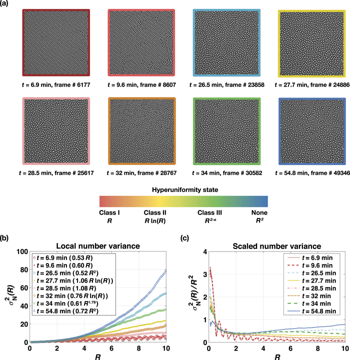
Figure 3. (a) Time-lapse microscope images show the changes in particle configuration while the crystal is disassembling. The image frames are coloured according to their hyperuniformity state as indicated in the colour-bar. (b) Local and (c) scaled number variance graphs measured through real-space sampling. The curves are coloured according to their hyperuniformity state as indicated in the colour-bar. Graph legends indicate the curve fitting functions.
Download figure:
Standard image High-resolution image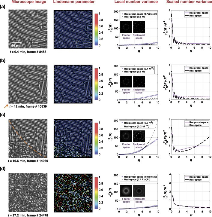
Figure 4. Microscope images (1st column), dynamic Lindemann parameter map (2nd column), local (3rd column) and scaled (4th column) number variance graphs obtained from reciprocal- (purple squares) and real-space (black dots) calculations show the effect of (a) various lattice imperfections, (b) small and (c) large inhomogeneities, (d) and statistically isotropic particle distribution on the system's hyperuniformity. The orange arrow shown in (b) points to the corner at which the crystal start disassembling. The orange dashed line shown in (c) artificially separates the two regions with solid- and liquid-like configurations. Graph legends indicate the curve fitting functions. Insets are Fourier and reciprocal space images of the corresponding number variance curves.
Download figure:
Standard image High-resolution imageTable 1. Best-fit function and fitting parameters of the real- and reciprocal-space number variance curves are provided for each frame presented in figures 3–10.
| Time | Frame # | # Particles | Real-space | Reciprocal-space | |||||
|---|---|---|---|---|---|---|---|---|---|
| Best fitting function | R-squared value | RMSE | Best fitting function | R-squared value | RMSE | ||||
| Figure 3 | 6.9 min | 6177 | 2105 | 0.526R | 0.629 | 1.02 | 0.570R ln(R) | 0.987 | 0.407 |
| 9.6 min | 8607 | 2027 | 0.602R | 0.844 | 0.610 | 0.760R ln(R) | 0.984 | 0.663 | |
| 26.5 min | 23858 | 1262 | 0.523R2 | 0.991 | 1.53 | 0.896R ln(R) | 0.991 | 0.585 | |
| 27.7 min | 24886 | 1028 | 1.06R ln(R) | 0.997 | 0.352 | 1.31R ln(R) | 0.994 | 0.707 | |
| 28.5 min | 25617 | 1016 | 1.08R | 0.975 | 0.406 | 1.02R ln(R) | 0.996 | 0.428 | |
| 32 min | 28767 | 963 | 0.755R ln(R) | 0.996 | 0.310 | 0.988R ln(R) | 0.998 | 0.278 | |
| 34 min | 30582 | 910 | 0.607R1.79 | 0.994 | 0.788 | 1.15R ln(R) | 0.998 | 0.346 | |
| 54.8 min | 49346 | 657 | 0.718R2 | 0.968 | 4.16 | 0.441R1.86 | 0.999 | 0.146 | |
| Figure 4 | 9.4 min | 8468 | 2028 | 0.614R | 0.844 | 0.704 | 0.665R ln(R) | 0.992 | 0.374 |
| 12 min | 10839 | 1988 | 0.632R | 0.818 | 0.790 | 0.392R1.93 | 0.998 | 0.386 | |
| 16.6 min | 14960 | 1710 | 0.0281R3.87 | 0.999 | 0.871 | 0.921R2 | 0.993 | 0.234 | |
| 27.2 min | 24478 | 1045 | 0.679R ln(R) | 0.967 | 0.750 | 0.909R ln(R) | 0.994 | 0.439 | |
| Figure 5 | (a) | — | 0.502R | 0.471 | 1.25 | 0.502R | 0.583 | 1.06 | |
| (b) | — | 0.487R | 0.471 | 1.22 | 0.861R2.57 | 0.999 | 3.49 | ||
| (c) | — | 0.0304R4.72 | 0.999 | 5.18 | 5.46R2.90 | 0.999 | 0.382 | ||
| (d) | — | 0.488R | 0.479 | 1.20 | 0.585R2.58 | 0.999 | 1.08 | ||
| (e) | — | No fit | — | — | 2.43R2.73 | 0.999 | 8.52 | ||
| (f) | — | 0.380R3.92 | 0.999 | 8.96 | 5.25R3.15 | 0.999 | 60.1 | ||
| Figure 6 | (a) | Leftmost | — | 0.360R3.27 | 0.999 | 4.21 | 0.620R | 0.659 | 0.814 |
| Middle | — | 0.008 70R4.22 | 0.999 | 0.772 | 1.06R2 | 0.991 | 3.23 | ||
| Rightmost | — | 0.305R | 0.555 | 0.646 | 0.297R | 0.889 | 0.259 | ||
| (b) | Leftmost | — | 0.333R3.23 | 0.999 | 3.96 | 0.633R | 0.719 | 0.747 | |
| Middle | — | 0.003 95R4.37 | 0.999 | 0.611 | 0.846R2 | 0.990 | 2.73 | ||
| Rightmost | — | 0.342R | 0.943 | 0.206 | 0.358R | 0.962 | 0.188 | ||
| (c) | Leftmost | — | 2.01R3.30 | 0.999 | 26.0 | No fit | — | — | |
| Middle | — | 0.0406R4.32 | 0.999 | 2.24 | 3.14R2.24 | 0.994 | 13.8 | ||
| Rightmost | — | 0.562R2 | 0.984 | 2.21 | 0.353R2 | 0.998 | 0.518 | ||
| Figure 7 | 10.3 min | 9258 | 2018 | 0.612R | 0.839 | 0.686 | 0.292R1.93 | 0.998 | 0.327 |
| 10.3 min | 9259 | 2014 | 0.591R | 0.864 | 0.602 | 0.827R ln(R) | 0.988 | 0.720 | |
| 10.3 min | 9265 | 2015 | 0.607R | 0.838 | 0.679 | 0.771R ln(R) | 0.986 | 0.641 | |
| Figure 8 | 8.9 min | 7967 | 2112 | 0.519R | 0.580 | 1.08 | 0.540R ln(R) | 0.984 | 0.430 |
| 9.1 min | 8006 | 1936 | 0.0157R3.5 | 0.996 | 0.921 | 0.426R2.03 | 0.998 | 0.630 | |
| 9.1 min | 8145 | 2025 | 0.340R ln(R) | 0.894 | 0.711 | 0.799R ln(R) | 0.988 | 0.593 | |
| Figure 10 | 28 min | 25184 | 1024 | 0.903R | 0.961 | 0.492 | 0.816R ln(R) | 0.999 | 0.169 |
| (b) | — | 0.258R + 0.0626R ln(R) | 0.993 | 0.0842 | 0.289R + 0.043R ln(R)+0.009R2 | 0.999 | 0.0210 | ||
| (c) | — | 0.840R−0.722 | 0.988 | 0.211 | 0.962R ln(R) | 0.989 | 0.676 | ||
| (d) | — | 0.824R + 0.118R ln(R) | 0.956 | 0.593 | 0.696R ln(R) | 0.998 | 0.196 | ||
| (e) | — | 1.06R ln(R) | 0.997 | 0.359 | 0.993R ln(R) | 0.997 | 0.380 | ||
Table 2. Best-fit function and fitting parameters of the real- and reciprocal-space number variance curves are provided for each frame described in the text, but not shown in the figures.
| Time | Frame # | # Particles | Real-space | Reciprocal-space | ||||
|---|---|---|---|---|---|---|---|---|
| Best fitting function | R-squared value | RMSE | Best fitting function | R-squared value | RMSE | |||
| 19.0 min | 17060 | 1637 | 0.0355R3.75 | 0.999 | 0.790 | 0.537R2.18 | 0.997 | 1.28 |
| 20.0 min | 18001 | 1552 | 0.0360R3.66 | 0.999 | 0.966 | 0.472R2 | 0.998 | 0.601 |
| 20.7 min | 18660 | 1499 | 0.0500R3.50 | 0.999 | 0.601 | 0.594R1.8 | 0.996 | 0.704 |
| 21.3 min | 19161 | 1467 | 0.0422R3.43 | 0.999 | 0.609 | 0.969R ln(R) | 0.989 | 0.712 |
| 25.0 min | 22506 | 1296 | 0.126R2.58 | 0.999 | 0.342 | 0.585R1.6 | 0.992 | 0.625 |
| 25.9 min | 23350 | 1275 | 0.179R2.43 | 0.999 | 0.415 | 0.797R ln(R) | 0.998 | 0.242 |
| 35.9 min | 32330 | 898 | 0.498R1.71 | 0.991 | 0.703 | 0.526R1.7 | 0.997 | 0.402 |
| 37.6 min | 33827 | 873 | 0.405R + 0.254R ln(R) | 0.997 | 0.150 | 0.414R1.8 | 0.999 | 0.170 |
| 38.0 min | 34228 | 865 | 0.699R ln(R) | 0.988 | 0.493 | 1.06R ln(R) | 0.998 | 0.263 |
| 43.4 min | 39044 | 788 | 0.617R1.7 | 0.997 | 0.441 | 0.593R1.75 | 0.997 | 0.502 |
| 43.7 min | 39368 | 787 | 0.592R2 | 0.986 | 2.12 | 0.624R1.6 | 0.996 | 0.447 |
| 43.8 min | 39440 | 786 | 0.250R2.38 | 0.999 | 0.444 | 0.396R1.94 | 0.999 | 0.291 |
| 62.6 min | 56329 | 616 | 0.0206R3.38 | 0.984 | 1.69 | 0.512R2 | 0.998 | 0.571 |
| 62.8 min | 56556 | 589 | 0.136R2.87 | 0.999 | 0.944 | 0.579R1.8 | 0.998 | 0.412 |
| 63.2 min | 56848 | 587 | 0.139R3.04 | 0.999 | 0.806 | 0.905R ln(R) | 0.991 | 0.587 |
| 64.5 min | 58056 | 575 | 0.0992R3.02 | 0.999 | 0.415 | 0.721R1.87 | 0.998 | 0.719 |
| 65.7 min | 59110 | 567 | 0.0618R3.08 | 0.999 | 0.708 | 1.30R ln(R) | 0.997 | 0.499 |
| 66.4 min | 59725 | 554 | 0.0830R2.92 | 0.994 | 1.45 | 0.567R1.88 | 0.997 | 0.685 |
| 66.9 min | 60207 | 545 | 0.0519R3.12 | 0.996 | 1.23 | 0.649R1.8 | 0.998 | 0.546 |
| 68.3 min | 61425 | 526 | 0.892R1.23(2 ⩽ R ⩽ 6) | 0.988 | 0.200 | 0.702R1.88 | 0.997 | 0.853 |
| — | — | — | 0.006 29R3.89(6 ⩽ R ⩽ 10) | 0.997 | 0.625 | — | — | — |
| video 1(frame # 39440) | ||||||||
| FOV | # Particles | Length (pixel) | Real-space | Reciprocal-space | ||||
| Best fitting function | R-squared value | RMSE | Best fitting function | R-squared value | RMSE | |||
| F0 | 200 | 360 | — | — | — | 0.995R | 0.954 | 0.598 |
| F1 | 207 | 360 | — | — | — | 1.25R ln(R) | 0.999 | 0.255 |
| F2 | 228 | 360 | — | — | — | 0.867R ln(R) | 0.999 | 0.0925 |
| 720 | 680 | 0.652R2 | 0.993 | 1.60 | 0.432R1.82 | 0.999 | 0.146 | |
| 786 | 720 | 0.250R2.38 | 0.999 | 0.444 | 0.396R1.94 | 0.999 | 0.291 | |
| 958 | 800 | 0.222R2.36 | 0.999 | 0.299 | 0.382R1.92 | 0.999 | 0.124 | |
| 1360 | 970 | 0.416R2 | 0.994 | 0.958 | 0.409R2 | 0.999 | 0.402 | |
The fitting functions are generated via the native least-square method-based curve fitting toolbox of Matlab. We assigned a hyperuniformity class to each structure by comparing the R-squared values of different fitting options. When the error values are close to each other (difference < 0.02), we choose the single parameter fit function. Small values of window radii are omitted when fitting the local number variance data, which is applied only to 2 ⩽ R ⩽ 10.
On a final note, while our real- and reciprocal-space analyses indicate disordered hyperuniformity when the crystal is disassembled, the corresponding static structure factor calculations at infinite wavelengths remain nonzero,  . In section 3.6 we discuss this issue and conclude that in a finite-sized experimental system with relatively fast dynamics,
  , by itself, cannot reliably diagnose the hyperuniformity.
3. Results and discussion
Figure 3 shows the dynamic evolution of hyperuniformity of a disassembling hexagonal colloidal crystal. Time-lapse microscope images of the system are given in figure 3(a). Corresponding local,  , and scaled,
  , number variance graphs calculated by the sampling of the real-space via circular observation windows are shown in figures 3(b) and (c), respectively. Different hyperuniformity classes are colour-coded. Dark red indicates strong hyperuniformity (class I) where number variance grows linearly as the window radius,
  . Dark blue indicates a non-hyperuniform state where number variance scales with the window surface area for two-dimensional space,
  . Shades of yellow-red denote logarithmic hyperuniformity (class II), where number variance grows logarithmically with the window radius,
  . Shades of green-blue indicate weak hyperuniformity (class III), where the number variance scales differently with the window surface area (less than the dimension of the system by α),
  .
.
3.1. Class I hyperuniformity when the laser is on
The system starts from a strong hyperuniform state (class I) for an almost perfect hexagonal crystal with only a few lattice imperfections (figure 3(a) and video 2, t = 6.9 min frame # 6177). Corresponding number variance curve shown in figure 3(b) grows linearly as the window radius,  , and scaled number variance (figure 3(c)) approaches zero while oscillating. On the other hand, fitting parameters given in table 1 indicate that the number variance curve calculated from the reciprocal-space behaves logarithmically,
  , pointing to a class II hyperuniform state. The reason is discussed in sections 3.2–3.5 with the aid of figures 4–9. We conclude that any lattice imperfections or inhomogeneities that break the system's periodicity will show up in the reciprocal-space calculations. Corresponding Fourier- and reciprocal-space images and the static structure factor confirm the periodic lattice configuration by the presence of intense Bragg peaks (video 2 and appendix figure 18).
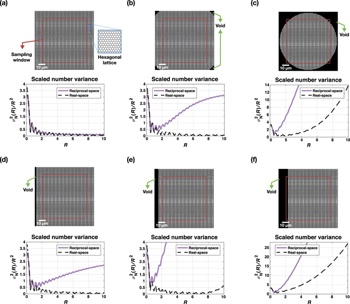
Figure 5. Numerical simulations show the effect of inhomogeneities on the system's hyperuniformity. (a) A hexagonal lattice formed by white disks tiling the entire field of view. (b) Black areas denote voids created by removing several white disks from the corners of the field of view. (c) Corner voids are extended into the sampling region. (d) The black line on the left is a void created by removing several white disks. (e) The thickness of the black line is increased towards the right of the field of view. (f) The black line is extended into the sampling region. Corresponding scaled number variance graphs are obtained from reciprocal- (purple squares) and real-space (black dots) calculations. Graph legends indicate the curve fitting functions.
Download figure:
Standard image High-resolution image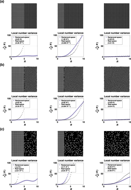
Figure 6. Numerical simulations show the influence of mixing configurations on the hyperuniformity. (a) Two hexagonal lattices formed by white disks with different interparticle distances tiling the two halves of the field of view (left). The lattice on the right is extended towards the left of the field of view (middle). The field of view is filled with a single hexagonal lattice (right). (b) A hexagonal lattice and a stealthy hyperuniform structure formed by white disks tiling the two halves of the field of view (left). The stealthy hyperuniform structure is extended towards the left (middle). The field of view is filled with the stealthy hyperuniform structure (right). (c) A hexagonal lattice and a disordered non-hyperuniform configuration formed by white disks are shown in the two halves of the field of view (left). The disordered non-hyperuniform configuration is extended towards the left (middle). The field of view is filled with disordered non-hyperuniform configuration (right). Corresponding scaled number variance graphs are obtained from reciprocal-(purple squares) and real-space (black dots) measurements. Graph legends indicate the curve fitting functions.
Download figure:
Standard image High-resolution image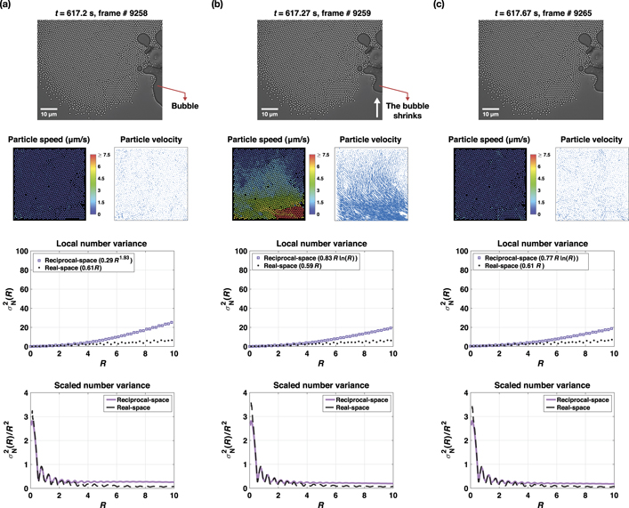
Figure 7. Time-lapse microscope images show a shrinking bubble boundary between (a) and (b), which creates a short-lived elastic vectorial fluid flow that terminates at (c). The vectorial flow is visualized on the particle speed and velocity maps shown in the 2nd row. Corresponding local (3rd row) and scaled (4th row) number variance graphs are obtained from reciprocal- (purple squares) and real-space (black dots) measurements. Graph legends indicate the curve fitting functions.
Download figure:
Standard image High-resolution image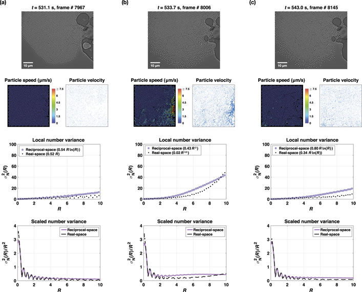
Figure 8. Time-lapse microscope images show a long-lived nonelastic vectorial fluid flow between (a) and (b) that terminates at (c). The vectorial flow is visualized on the particle speed and velocity maps shown in the 2nd row. Corresponding local (3rd row) and scaled (4th row) number variance graphs are obtained from reciprocal- (purple squares) and real-space (black dots) measurements. Graph legends indicate the curve fitting functions.
Download figure:
Standard image High-resolution image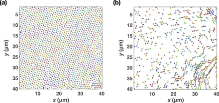
Figure 9. Particle trajectories under (a) elastic fluid flows shown in figure 7, and (b) nonelastic fluid flows shown in figure 8. The initial coordinates of the particles are denoted by circles. All the particles in the field of view are tracked within the frame range of 9258–9265 in (a), but 500 randomly chosen particles are tracked within the frame range of 7967–8145 (b) to simplify an otherwise too crowded image.
Download figure:
Standard image High-resolution image3.2. Switching between class I, class II, and non-hyperuniform states when the laser is off
Video 2 shows persistent hyperuniformity of the crystal until t = 8.9 min frame # 7967 at which the laser is turned off. Right at this moment, the lattice suddenly relaxes, interparticle distances grow, and several lattice imperfections emerge and propagate, as clearly seen from the dynamic Lindemann parameter map of figure 4(a) and video 2. This is also reflected in the packing fraction graph of video 2 and appendix figure 14 with a sudden drop from ϕ ∼ 0.84 to ∼0.78, which briefly recovers to ∼0.81, but continues to drop since the crystal is disassembling. There are three gaps in this graph, corresponding to the gaps in data acquisition, as discussed in section 2.1.
The underlying cause of the emergent lattice imperfections is strikingly visual in the particle speed and velocity maps. The formation of vectorial flows in various directions results in increased activity in particle displacement and speed profiles. As will be discussed in section 3.5 with the aid of figures 7–9, despite such strong perturbations, the lattice's overall periodicity is preserved, which is confirmed via Fourier image and power spectrum analyses shown in video 2 and appendix figure 18.
As a result of these vectorial flows, hyperuniformity is temporarily lost (video 2 and figures 7 and 8) as the density fluctuations scale with the window surface area and the tail of the scaled number variance curve flattens (converges to a nonzero value) for large window radii (R > 6). The hyperuniformity is recovered shortly (9 < t < 11 min), where real- and reciprocal-space analyses point to class I and class II hyperuniform states, respectively. Representative curves for t = 9.6 min (frame # 8607) are given in figures 3(b) and (c) with their fitting parameters in table 1. Corresponding Fourier- and reciprocal-space images and the structure factor in appendix figure 18.
At around t = 11 min of video 2, it is seen that the crystal disassembles starting first from the lower-left then the lower-right corners, which is also shown in figure 4(b). This is also evident in the particle speed and velocity maps.
3.3. Peculiar density fluctuations at real- and reciprocal-space analyses in the presence of inhomogeneities
The peculiarities in density fluctuations start around t = 12 min. Real-space calculations indicate a class I hyperuniformity,  , until t = 14 min whereas reciprocal-space calculations point to a non-hyperuniform state,
  . At around t = 17 min half of the field of view is solid-like, the other half is liquid-like (video 2 and figure 4(c)). As expected, such a significant inhomogeneity in spatial particle distribution results in a complete loss of hyperuniformity in both number variance calculations. The inhomogeneities are also reflected in the Fourier- and reciprocal-space images with the emergence of additional but weaker peaks (insets of figure 4(c)).
We performed numerical simulations to clarify the effect of inhomogeneities on hyperuniformity. Figure 5(a) shows the scaled number variance graph of a perfect hexagonal crystal formed by white disks tiling the entire field of view. We introduce voids starting from the corners by removing several disks (figure 5(b)). This action does not affect the number variance calculated through real-space sampling. However, reciprocal-space calculations are immediately affected by this action and show complete loss of hyperuniformity.
The reason for this disagreement is purely geometrical. The observation windows are circular, and the field of view is square (figure 2(b)). These windows cannot sample the corners of the field of view. Consequently, they do not 'see' the voids unless they are extended towards the sampling region (figure 5(c), red square). In contrast, the reciprocal-space calculations immediately detect these voids and loses hyperuniformity since the Fourier calculation effectively projects the real-space onto a torus where the voids overlap and create a large space devoid of white disks.
Figure 5(d) shows a line version of the artificial lattice imperfections directly detected by the reciprocal-space calculations. In contrast, the real-space number variance curve is unaffected by it despite the observation windows having large radii that can sample from the sides of the field of view and 'see' this relatively thin black line (figure 2(b)). However, the line is not sampled by the majority of the windows, and statistically, this imperfection has a negligible effect on the number variance calculations. If we increase the thickness of this line (figure 5(e)) real-space calculations also lose hyperuniformity for large window radii, R > 8. Further increase of the line thickness (figure 5(f)) results in a complete loss of hyperuniformity for real- and reciprocal-space calculations.
The system regains its hyperuniformity at around t = 27 min once the particles are distributed isotopically throughout the system (figure 4(d)). Real- and reciprocal-space calculations both point to the logarithmic, or class II hyperuniformity. Representative number variance curves for t = 27.7 min (frame # 24886) are given in figures 3(b) and (c), and the fitting parameters in table 1. Corresponding Fourier- and reciprocal-space images and the structure factor in appendix figure 18. However, before this happens, video 2 and tables 1 and 2 show an early recovery of hyperuniformity for the reciprocal-space calculations starting at around t ∼ 20 min. Although interparticle distances are clearly non-uniform during 19 < t < 27 min, the power spectrum number variance calculations detect an overall degree of order in the system.
In order to verify this, we performed three numerical simulations where the field of view is divided into two halves. First, both halves are tiled with hexagonal lattices with different interparticle distances (figure 6(a)). Second, one half is tiled with a hexagonal lattice and the other with a disordered stealthy hyperuniform configuration (figure 6(b)). Third, one half is tiled with a hexagonal lattice and the other with a disordered non-hyperuniform configuration (figure 6(c)). Then, the area occupied by the right-hand-side configuration is advanced towards the left-hand-side and eventually fills the entire field of view.
In the first simulation, real- and reciprocal-space calculations point to non-hyperuniform and strongly hyperuniform configurations, respectively (figure 6(a), left). As expected, only the reciprocal-space calculations successfully detected the orderliness of the two halves and confirmed the multi-hyperuniformity of the overall configuration. However, when the areas occupied by the two halves are not equal, in other words if the density variations are large, reciprocal-space calculations also indicate a non-hyperuniform behaviour (figure 6(a), middle). This is similar to the strong inhomogeneity case shown in figure 4(c). When a single hexagonal lattice fully occupied the field of view, both calculations point to a strong, class I hyperuniform state (figure 6(a), right).
The second simulation also confirms these observations with two periodic configurations (figure 6(b)). The third simulation further verifies that if one half of the field of view is filled with a non-periodic, non-hyperuniform configuration, then both calculations point to a non-hyperuniform state at all times (figure 6(c)). In light of these simulations and the power spectrum analyses shown in video 2, we conclude that the particle configurations at 19 < t < 27 min are indeed ordered despite the apparent non-uniform interparticle distances with small density variations.
The conclusion drawn from this sub-section is that real- and reciprocal-space number variance calculations are both necessary and complementary to each other to correctly ascertain the hyperuniformity of a driven dissipative system.
3.4. Oscillations between class II, class III, and non-hyperuniform states for a disordered configuration
Once the system reaches a statistically isotropic particle distribution, real-space calculations show a brief class I behaviour (at t = 28.5 min frame # 25617), then switch to class II (at t = 32 min frame # 28767) and class III (at t = 34 min frame # 30582) hyperuniform states. Finally, after t = 43.7 min, real-space calculations indicate an irrecoverable non-hyperuniform state as the particles are distancing from each other (tables 1 and 2). Also, we suspected that there is an insufficient number of particles within the field of view to perform reliable real-space hyperuniformity analyses. To test this, we changed the size of our field of view (FOV) for the particle configurations observed at time t = 43.8 min and frame # 39440 (appendix figure 19(a)). The original FOV size is changed from 720 × 720 pixels to a smaller FOV with 680 × 680 pixels and larger FOVs with 800 × 800 and 970 × 970 pixels. The sampling region is kept constant at Rmax = 10 μm. Real- and reciprocal-space number variance analyses are presented in table 2, which shows even if the number of particles are increased twice for the FOV size of 970 × 970 pixels, real-space measurements points to the non-hyperuniform configuration.
In addition to the real-space measurements, we also tested the accuracy of our reciprocal-space measurements. We further divided the original FOV to four nonintersecting FOVs with 360 × 360 pixels (appendix figure 19(b)). We measured the reciprocal-space number variance in the quadrants shown in appendix figure 19(b) for Rmax > 10 μm, which corresponds to approximately half of the side length. The results provided in table 2 show that the FOV sizes larger than the original FOV do not significantly change the reciprocal-space number variance measurements. However, the FOV sizes much smaller than the original FOV leads to artificial class I or class II hyperuniform states for reciprocal-space measurements. Therefore, we conclude that our original FOV size is sufficient to draw reliable conclusions from the reciprocal-space measurements.
A temporary loss of hyperuniformity for reciprocal-space calculations between 32.4 < t < 32.7 min (frames 29202 to 29451) is due to the detection error for particles at the upper corner of the field of view, which temporarily appear darker with respect to the others. This error can be seen through the dynamic Lindemann parameter map. We note that this frame span is the only such incident throughout video 2. We further note that in figures 4–6, and tables 1 and 2, the density fluctuations scale as  with x > 2, only in the presence of strong inhomogeneities in the system. This is because x = 2 equality only holds for homogenous particle configuration in two-dimensional space.
In contrast to real-space calculations, reciprocal-space calculations continue to show oscillating hyperuniformity between class II and class III states until t ∼ 65 min, and afterwards exhibit only class III hyperuniformity until the end of the video (see figures 3(a) and (b), and tables 1 and 2). This is also reflected in the power spectrum analysis shown in video 2, which indicates a relatively weak periodicity in the particle configuration. To understand this, we analysed the initial frames of the experimental video, right after the sample preparation step and before we turned on the laser for the first time. We repeat this for several experiments. The results for the experiment we report here are shown in the appendix figure 20, where the reciprocal-space image and the structure factor are pointing at a random particle configuration with no periodicity, noticeably different than those seen at the end of video 2.
In our previous study [42], we studied the aggregation mechanism of this particular system. We showed that various interaction mechanisms specific to different particles (CdTe quantum dots and polystyrene particles) and living organisms (E. coli and M. luteus bacterial cells and yeast and human cells) are negligible. In fact, the dominant mechanisms are hydrodynamic and hard-sphere in origin. Therefore, we suspect that the lingering hyperuniformity in this driven dissipative system, long after the absence of an external energy source, may be related to the mutual coupling of the particle positions and velocities with the flow fields.
3.5. Robust hyperuniformity against vectorial fluid flows
The hyperuniformity of the system is remarkably robust against random vectorial flows, which can be elastic or nonelastic as well as short or long-lived. Figures 7 and 8 displays time-lapse microscope images during elastic and nonelastic flows, respectively. In elastic flows, the particles do not change their original positions (figure 9(a)), while nonelastic flows sweep clusters of particles and change their original positions (figure 9(b)). New particles then replace these empty sites. Regardless of these differences, the system's hyperuniformity recovers once these flows diminish.
A shrinking bubble boundary forms a short-lived vectorial fluid flow, which can be observed through the particle speed and velocity maps shown in figure 7 and video 2. Despite the apparent inhomogeneities in particle speeds and velocities, the number variance curves are not significantly affected by such flow fields. Similarly, prolonged vectorial flows shown in figure 8 increase the density fluctuations, but then hyperuniformity recovers once they vanish. The flows shown in these particular examples are representative of many similar vectorial flows seen throughout video 2. We believe that the oscillations of the number variance curves observed throughout video 2 are due to perturbations from such short-lived and prolonged vectorial flows.
The robustness of the system's hyperuniformity against various external perturbations directly results from its internal dynamics. As we explained in detail in references [41, 42], the entire system is mutually coupled through intrinsic positive and negative feedback mechanisms. Fluid flows change the particle positions and velocities, and in return, rearrangement of the particles modify the flow field. This is why several lattice imperfections emerge and propagate but do not significantly change the lattice's overall periodicity. Of course, there are limits to such self-correction mechanisms since eachconfiguration has a finite basin of attraction in the phase- and real-space. Sufficiently large spatiotemporal perturbations may well reconfigure the entire system [41]. However, this is not the case in the experiments provided here since the laser was turned off and we have not actively modifying the system dynamics as we previously did in references [41, 42].
3.6. Nonzero static structure factor value at infinite wavelengths for disordered hyperuniform states
In the previous sub-sections, we provided evidence of several hyperuniformity classes through real- and reciprocal-space measurements. Although anomalous suppression of density fluctuations is observed for disordered particle configurations, their structure factor values remain nonzero at infinite wavelengths,  . This contradicts the hyperuniformity description established for infinitely large systems,
  [2].
[2].
Observation of a positive value for structure factor at long wavelengths is not new; it has been reported previously for several experimental systems [6, 26, 53]. It has been argued that the finite size of an experimental system prevents achieving  , even when the system presents clear signatures of hyperuniformity. Dreyfus et al came to the conclusion that reciprocal-space measurements fail to diagnose the hyperuniformity of an experimental disordered jammed soft polydisperse particles, where real-space measurements are deemed more reliable [6]. Berthier et al confirmed the hyperuniformity of a jammed packing of size-disperse spheres by looking at the vanishing isothermal compressibility instead of the static structure factor [26].
In addition to the finite size effects, the effects of finite-resolution of particle positions, experimental and measurement noise, imperfections in optical imaging, image size restrictions, and size polydispersity are also pointed out as difficulties to diagnose the hyperuniformity of an experimental system directly from structure factor analysis [6, 26]. Admittedly, all these effects limiting the potential of an experimental system accessing to small k values are also present, to some extent, in our experimental system, except size polydispersity. However, unlike in previously reported cases, our real- and reciprocal-space measurements mostly agree on this particular system's hyperuniformity. Earlier studies measure hyperuniformity directly from the power spectrum. In addition to this, here we also provide the number variance of the power spectrum (4). This fact, together with our results discussed in the previous sections led us to conclude that both measurements have their merits. Real- and reciprocal-space number variance measurements complement each other and should be used together to assess the hyperuniformity of a given experimental system correctly.
We believe that the physical reason for the agreement of our dual approach on the system's hyperuniformity is the mutual coupling of the entire system, as pointed out in the previous sub-section. Further, the positive structure factor value for small k values is likely due to the Brownian motion of the particles and structural defects produced by their random collisions in our experiment.
We tested both of these hypotheses with numerical simulations. The results are presented in figure 10. A dynamic Lindemann parameter map of the experimental frame at t = 28 min (frame #25184), the corresponding scaled number variance curves, and the structure factor are shown in figure 10(a). The real- and reciprocal-space calculations point to a class I and class II hyperuniform states, respectively with  . In figure 10(b), we show the same analyses for a simulated stealthy hyperuniform structure exhibiting class I hyperuniformity with
  . Next, we introduce Brownian noise to each particle in the stealthy configuration (figure 10(c)), for which the number variance curves indicate a class II hyperuniform state with
  . Noticeably, the peaks at k > 5 vanish, pointing to the presence of only short-range interparticle correlations. We then introduce several structural defects without the Brownian noise (figure 10(d)), which, again, results in a class II hyperuniform state with
  . Lastly, we include both Brownian motion and structural defects (figure 10(e)). The system exhibits a class II hyperuniformity with
  . The corresponding structure factor graph similarly indicates short-range interparticle correlations as in figure 10(c).
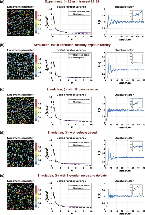
Figure 10. The behaviour of nonzero structure factor at long wavelengths in a dissipative system. Dynamic Lindemann parameter maps (1st column), scaled number variance graphs obtained from reciprocal- (purple squares) and real-space (black dots) measurements (2nd column), and the static structure factor graphs (3 column) are provided for the experiment (a), numerically simulated stealthy hyperuniform structure (b), with addition of only Brownian motion (c), with addition of only structural defects (d), with addition of Brownian motion and structural defects (e). Scaled number variance graphs are obtained from reciprocal- (purple squares) and real-space (black dots) measurements. Graph legends indicate the curve fitting functions.
Download figure:
Standard image High-resolution image
Figure 11. (a) Time-lapse microscope images show the changes in particle configuration while the crystal is disassembling. The image frames are coloured according to their hyperuniformity state as indicated in the colour-bar. (b) Local and (c) scaled number variance graphs calculated through real-space sampling. The curves are colour-coded according to the colour-bar to describe their hyperuniformity state. Graph legends indicate the curve fitting functions.
Download figure:
Standard image High-resolution image
Figure 12. A screenshot of the toolbox showing its components: the 1st row shows from left to right the microscope image, dynamic Lindemann parameter map, and the plot showing time evolution of the packing fraction. The 2nd row shows from left to right the particle speed map, particle velocity map, the Fourier and reciprocal-space images. The 3rd row shows from left to right the plots of local and scaled number variances, and the static structure factor.
Download figure:
Standard image High-resolution imageWe believe the Brownian motion of the particles and the structural defects produced by their collisions is sufficient to explain the positive structure factor for small k that we observe experimentally. We also showed that the structure factor of the experiment showing oscillating peaks indicating long-range particle correlations, which are likely preserved thanks to the nonlocal interactions ensured by the flow fields.
4. Conclusions
The experimental study presented here is uniquely different from previous experimental and numerical studies in several key aspects.
Firstly, almost all reported studies started from a disordered non-hyperuniform configuration that converged to a hyperuniform structure by transitioning from an active to an absorbing state, and in some cases to an active steady state [6, 7, 24–40]. On the contrary, our experiments started from an ordered state, which transitioned to a series of disordered hyperuniform states. The particles were always active and continuously colliding with each other. Our system was never jammed, nor did it converge to absorbing or active steady states.
Secondly, our system experienced numerous random external perturbations and was subjected to strong inhomogeneities. The particle configurations changed continuously, and each configuration was analysed with a single measurement (no ensemble averaging was performed).
Next, the particle positions and velocities are mutually coupled to the fluid flow through an internal feedback mechanism. We postulate that this feedback mechanism renders the system's hyperuniformity robust against otherwise detrimental effects such as, imperfections, noise, fluctuations, random perturbations, and inhomogeneities.
Lastly, we analysed all these conditions on-the-fly together with their impact on the system's hyperuniformity by utilizing a comprehensive computational toolbox. This allowed us to show, for the first time, the real-time dynamic evolution of hyperuniformity in a driven dissipative system. Further, it provided the evidence of a prolonged hyperuniformity in a driven dissipative system even long after the external energy input has been removed.
We speculate that the potential role of these internal feedback mechanisms on the hyperuniformity may not be limited to our specific system, but it may be commonly encountered in other driven dissipative systems.
Acknowledgments
This work received funding from the European Research Council (ERC) under the European Union's Horizon 2020 research and innovation programme (Grant agreement No. 853387), TÜBİTAK-EC Marie Skłodowska-Curie Actions Co-fund program (Grant agreement No. 120C074), TÜBİTAK (Grant agreement No. 115F110 and No. 20AG001). The authors thank Satya N Majumdar of LPTMS, CNRS and Université Paris-Sud (Orsay) for inspiring this work. ÜSN, GM, MB, SSK, and DV developed the computational toolbox and analysed the data. ED, EES, and SG performed the experiments. SH, MHG, EY, ÜSN, MB, and SSK performed the numerical simulations. SI initiated the project, supervised the research, and wrote the article.
Data availability statement
The data that support the findings of this study are available upon reasonable request from the authors.
Appendix
See figures 11–20 and table 3.
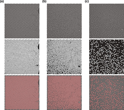
Figure 13. The detection output at different stages of three randomly selected frames (a)–(c). The 1st row shows the original video frames. The 2nd row shows the processed frames after gray-level adjustment and the dilation operators. The 3rd row shows the detection results as red circles overlaying the original video frames. The red circles are numerically stored as the centers of the detected particles.
Download figure:
Standard image High-resolution image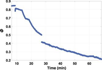
Figure 14. Plot showing the time evolution of the packing fraction.
Download figure:
Standard image High-resolution image
Figure 15. Graphs show log–log plots of local number (top) and scaled volume (bottom) fraction variance curves for (a) the experimental frames shown in figures 3(a) and (b) for the numerically simulated hexagonal lattice to which several lattice defects are introduced with increasing percentages. The dashed straight lines shown in the graphs correspond to a theoretical class I (red) and class III (pink) hyperuniform states. Experimental number and volume fraction variance curves shown in (a) gives similar estimation of hyperuniformity for a given configuration. However, local volume fraction calculations seem to be more sensitive to the structural defects present in the system. The confirmation is provided through numerical simulations (b), where local number and volume fraction variance are calculated in the presence of structural defects with varying degrees.
Download figure:
Standard image High-resolution image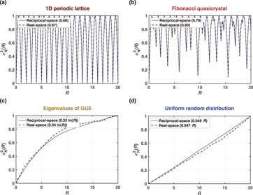
Figure 16. The plots show real- and reciprocal-space local number variance measurements for different 1D simulation cases agree. The reciprocal-space measurements are done after setting the 1st and 2nd values of the static structure factor equal to the third value. To appreciate the difference between the real- and reciprocal-space number variance curves, we normalized all curves to have their maximum value equal to 1. For all systems, the size and the maximum observation window radius are set to be L = 10 000 and Rmax = 20. The simulated point distributions represent (a) a periodic lattice of N = 5000 points, (b) a Fibonacci quasicrystal with N = 4182 points, (c) the distribution of N = 254 eigenvalues (10% interval of the central eigenvalues) of a single 2000 × 2000 random matrix from a Gaussian unitary ensemble (GUE), and (d) uniform random distribution of N = 5000 points along a line. Fitting functions are given in the legends, where the number variance is known to be constant for (a) and (b) for which a running average was used. The fits for (c) and (d) are optimized to be proportional to ln(R), R1–α , or R for class II, III, or non-hyperuniform states, respectively.
Download figure:
Standard image High-resolution image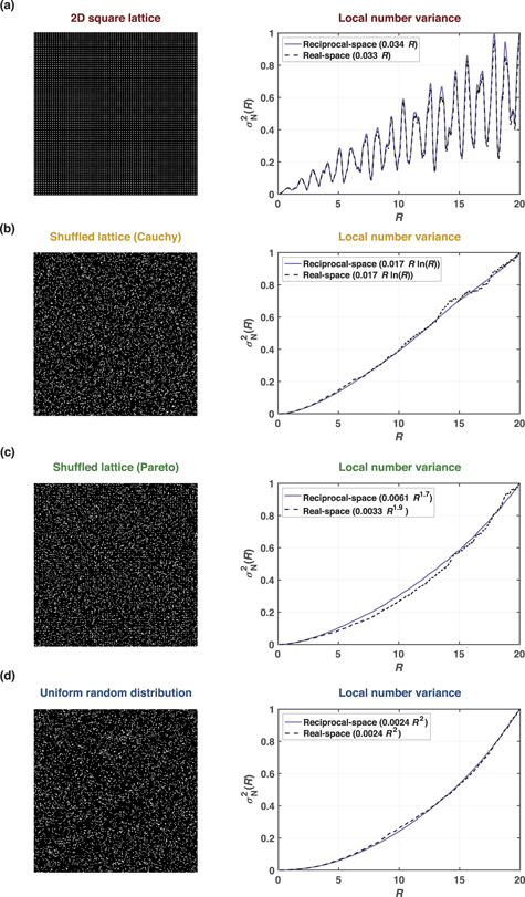
Figure 17. The plots show real- and reciprocal-space local number variance measurements for different 2D simulation cases agree. The reciprocal-space measurements are done after setting the 1st and 2nd values of the structure factor equal to the 3rd value. To appreciate the difference between the real- and reciprocal-space number variance curves, we normalized all curves to have their maximum value equal to 1. For all systems, the side length, maximum observation window radius, and the number of points are set as L = 150, Rmax = 20, and N = 5625 (except for (d) in which the number of points is set as N = 5000). The simulated point distributions represent (a) a square lattice with a lattice parameter size Lc = 2, (b) and (c) the same square lattice as in (a) with additional perturbations in the form of a random displacement applied to every point. The displacement is sampled from a Cauchy distribution (expected to result in class II) with γ = 0.5 Lc for (b), and from a Pareto distribution (expected to result in class III) with scaling parameter xm = 1/6 Lc and shape parameter a = 2/3 for (c) and (d) the random uniform distribution of points. Fitted functions are given in the legends, where the optimal fit is found to be proportional with either R, R ln(R), R2–α , or R2, corresponding to class I, II, III, or non-hyperuniform states, respectively.
Download figure:
Standard image High-resolution image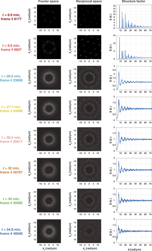
Figure 18. Fourier and reciprocal space images, and the static structure factor measurements of the selected frames presented in figure 3. The frame numbers and the corresponding times are given in the leftmost column. According to the colour-bar, the labels are colour-coded, which is given in figure 3.
Download figure:
Standard image High-resolution image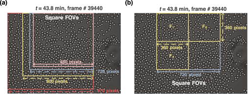
Figure 19. (a) The pictorial representation of field of views (FOVs) with different sizes for the particle configuration seen at time t = 43.8 min and frame # 39440. The side length of the square fields of view are specified on each figure. The blue square is the FOV used in the original manuscript. (b) The pictorial representation shows division of the original FOV of 720 × 720 pixels to four nonintersecting FOVs with 360 × 360 pixels for the particle configuration seen at time t = 43.8 min and frame # 39440.
Download figure:
Standard image High-resolution image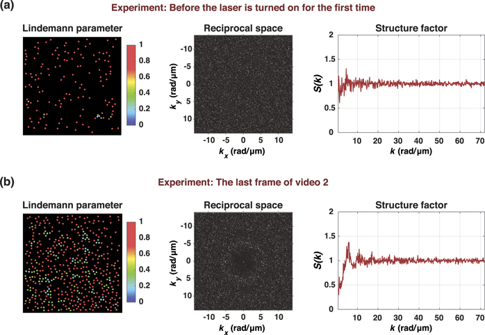
Figure 20. Dynamic Lindemann map (left), reciprocal-space image (middle), and the static structure factor calculations (right) for (a) the initial configuration of the experimental system before the laser is turned on for the first time, and (b) the final configuration of the experimental system (frame # 61425). The static structure factor and the reciprocal space images for initial configuration indicates a random non-hyperuniform configuration. On the contrary, a dark disk-like region at the centre of the reciprocal space, which is translated into a drop in the value of the structure factor for the final video frame along with the data shown in table 2 points to a weak, remnant hyperuniformity.
Download figure:
Standard image High-resolution image
Table 3. Best-fit function and fitting parameters of the real- and reciprocal-space number variance curves are provided for the additional experiment shown in appendix figure 11.
| Time | Frame # | # Particles | Real-Space | Reciprocal-Space | ||||
|---|---|---|---|---|---|---|---|---|
| Best fitting function | R-squared value | RMSE | Best fitting function | R-squared value | RMSE | |||
| 17.6 min | 15795 | 2055 | 0.814R | 0.810 | 1.08 | 0.631R ln(R) | 0.985 | 0.516 |
| 26.4 min | 23779 | 2059 | 0.699R | 0.779 | 0.974 | 0.522R ln(R) | 0.982 | 0.456 |
| 27.9 min | 25117 | 2014 | 0.488R ln(R) | 0.925 | 0.877 | 0.559R ln(R) | 0.990 | 0.361 |
| 29.0 min | 26067 | 1930 | 0.0676R2.77 | 0.997 | 0.635 | 0.299R2 | 0.998 | 0.372 |
| 32.3 min | 29105 | 1717 | 0.0219R3.48 | 0.997 | 1.04 | 0.534R2 | 0.993 | 1.30 |
| 35.6 min | 32067 | 1587 | 0.0302R3.24 | 0.997 | 0.774 | 0.299R2 | 0.998 | 0.315 |
| 40.1 min | 36067 | 1494 | 0.0102R3.61 | 0.992 | 1.02 | 0.320R2 | 0.999 | 0.308 |
| 44.9 min | 40391 | 1431 | 0.0216R3.31 | 0.996 | 0.765 | 0.319R1.85 | 0.999 | 0.0681 |
| 48.2 min | 43391 | 1374 | 0.0446R2.77 | 0.994 | 0.580 | 0.588R ln(R) | 0.999 | 0.122 |
| 49.4 min | 44391 | 1342 | 0.817R | 0.962 | 0.378 | 1.09R ln(R) | 0.993 | 0.597 |
| 50.0 min | 44991 | 1312 | 0.392R ln(R) | 0.956 | 0.474 | 0.680R ln(R) | 0.998 | 0.204 |
| 50.1 min | 45081 | 1317 | 0.798R | 0.970 | 0.374 | 0.605R ln(R) | 0.997 | 0.204 |
| 52.3 min | 47056 | 1184 | 0.144R2.34 | 0.992 | 0.751 | 0.376R1.94 | 0.999 | 0.132 |