

Abstract
By means of the Monte Carlo method, a numerical study of the vortex system in a high-temperature superconductor under the impact of pulses of magnetic field has been conducted. Various shapes and amplitudes of pulses have been considered. Samples with random and regular distributions of three different numbers of defects have been compared from the viewpoint of efficiency of flux trapping. The low-temperature behavior of vortices and their penetration into samples have been shown to be independent of the pulse shape but strongly dependent of the type of pinning distribution. Saturating dependences of density of trapped magnetic flux on the pulse amplitude have been obtained. The samples with random pinning demonstrated higher efficiency of flux trapping at lower pulse amplitudes, and the samples with a triangular lattice of defects—at higher amplitudes. If the amplitude exceeded the saturation field of both samples, the trapped field was almost equal. The increasing number of defects has lead to an increase in trapped field within the considered range of concentrations.
Export citation and abstract BibTeX RIS
1. Introduction
The interest in studying the magnetic properties of high-temperature superconductors (HTSs) is growing every year. Numerous studies have shown that bulk superconductors and stacks of HTS tapes are capable of trapping magnetic fields of several teslas or higher and can therefore be used as pseudo-permanent trapped field magnets (TFMs) [1–18]. The range of potential practical applications of such magnets extends from magnetic bearings and levitation devices to motors and high-field magnets [1, 2, 16, 19–23]. For example, TFMs made from magnetized stacks of HTS tapes have been shown to provide higher levitation forces compared to bulks [24], whereas bulk HTSs look very promising for the development of compact high-torque rotating machines [18].
Two main techniques are used to magnetize superconductors today: field cooling (FC) and pulsed-field magnetization (PFM). The former is a static method that facilitates the material's field trapping potential to its fullest. However, it requires large magnets and is very energy-consuming [16]. The PFM method, on the other hand, is relatively compact and costs less, but more importantly, it allows to magnetize a superconductor within tens of milliseconds [1, 2]. Nevertheless, despite a lot of theoretical and experimental research being done to develop and improve this method, the trapped magnetic fields provided by PFM are still much lower than those obtained through FC, especially at low temperatures [1–3, 8, 9].
The majority of practically applicable superconductors are type-II superconductors in which a transition to a mixed (vortex) state occurs in a wide range of magnetic fields and currents. The phase states and dynamics of vortices determine the transport and magnetic properties of HTSs in this state. In fact, vortices emerge in various systems such as bulk superconductors, stacks of HTS tapes, Josephson junctions, and superconducting bridges (larger than the coherence length ξ but smaller than the magnetic field penetration depth λ), and they are of great interest for research. For example, many studies are devoted to the so-called proximity vortices appearing in various systems with weak coupling. Those are, for example, the superconductor–ferromagnet–superconductor (S/F/S) junctions [25] (and the more complex S–Ho/N/Ho–S contacts [26] where N is the normal (non-superconducting) phase), the S/TI/S (where TI stands for topological insulator) [27] and S/Ws/S (where Ws is the Weyl semimetal) [28] contacts, as well as elliptical annular junctions [29, 30]. Recent studies have shown that anharmonic relations between the supercurrent and phase occur in junctions with strong Josephson coupling, causing the vortices to increase in size [31–33]. In all the mentioned cases, circular currents with normal centers appeared in the non-superconducting phase. The junction thickness and properties of the normal layer determined the number and positions of the emerging vortices. In superconducting bridges [34], with the simultaneous presence of transport current and magnetic field, various vortex regimes have been observed, including the so-called kinematic vortices (vortex–antivortex pairs) appearing at currents exceeding the decoupling current. In the case considered in our paper (and in [1–18]), when a type-II superconductor much larger than λ is placed in an external magnetic field (much less than the upper critical field), the Abrikosov vortices are observed. These are long thin cylinders of normal phase of radius ∼ξ encircled by a supercurrent flowing at a distance ∼λ and carrying a single quantum of magnetic flux Φ0.
As has been demonstrated in numerous papers devoted to the pulsed magnetization of HTSs, a rapid change in the external magnetic field leads to a strongly nonequilibrium motion of magnetic flux [3, 12, 16, 17]. When the magnetic field exceeds a certain threshold, vortices suddenly begin to move in large quantities and occupy the sample center. This process is called the flux jumps or flux avalanches (‛giant field leaps' in [16]). Such rapid motion of the magnetic flux causes significant local heating and energy losses. Consequently, the local critical current density of the material decreases, and the HTS traps less field. It has been recently shown in [35] that flux jumps in bulk HTSs can even cause damage to the material due to cracking induced by thermal and electromagnetic strain. The negative influence of flux jumps becomes more significant with the increasing field ramp rate or the decreasing ambient temperature. On the other hand, some recent studies have shown that nonequilibrium vortex dynamics can facilitate pulsed magnetization and even improve field-trapping efficiency if multi-pulse methods are used [11, 12].
The number of various parameters that can influence the pulsed magnetization is vast [1, 2, 5, 9, 17]. It is necessary to consider the shape, magnitude, duration, and number of applied magnetic pulses. One should also mind the temperature regime and pinning properties of the material under study when dealing with flux jumps. The problem of selecting the optimal parameters is thus quite relevant but very complicated at the same time. Numerical modeling can be a convenient tool for this purpose. Its primary advantage is the possibility of calculating the dependence of, e.g., the trapped field on one particular parameter while keeping the others fixed (which is practically impossible in experimental studies due to the imperfection of samples and experimental conditions). There are various modeling techniques for studying the transport and magnetic properties of HTSs [1, 2, 5–7, 12, 36–38]. For example, the Monte Carlo method makes it possible to explicitly model the behavior of Abrikosov vortices in a wide range of magnetic fields, transport currents, and temperatures, as well as consider the various possible distributions and types of defects [36–44]. Since the vortex dynamics makes the main contribution to the magnetization of HTSs, this method can become a powerful tool for finding ways to quantitatively and qualitatively improve the trapped field during PFM.
In our previous work [44], we studied the effects arising during magnetization of a HTS using a linearly increasing external magnetic field with various ramp rates. We demonstrated some vortex behavior features which manifested as rapid jumps of the averaged magnetic field inside the material, very similar to flux jumps described in papers [11, 12, 16, 35]. These features occurred due to the emergence of a potential barrier near the sample boundaries and its subsequent breakdown with the rising external magnetic field. We showed that the threshold field (also called the activation field in [17]) at which the flux jumps occurred depended on the number of defects and the type of their distribution over the sample (as did the amplitude of jumps).
In the present work, we were pursuing answers to the following questions. Would the flux jumps manifest similarly for the cases of linear and non-linear magnetization? Would they reappear during consecutive magnetization and demagnetization of samples (in other words, would the near-edge potential barrier emerge in samples already containing trapped flux)? Another important task was to study how the various pulse shapes and amplitudes influenced the flux trapping efficiency (and how the trapped field depended on flux jumps). Finally, we wanted to observe the effect of variously shaped pulses on the trapped field homogeneity.
This paper is organized as follows. Section 2 describes the computational method, the model used for calculations, and the sample parameters. The main results of simulations are given in section 3. Section 4 discusses the obtained results and provides some speculations on how they can be explained. The major conclusions are drawn in section 5.
2. Simulation model and parameters
Simulations of the vortex behavior were done for the model of a layered HTS using the continuous-space Monte Carlo method. This method has already been successfully applied before [36–48] in our studies of the magnetic and transport phenomena in HTSs. Using these simulations, we have been able to investigate the effect of anisotropy [39–41], point defects and ferromagnetic nanoparticles [37–39, 44, 47], antidots [43], and strain [42] on the magnetization and critical current of layered HTSs as well as the phase and dynamic states of the vortex system.
The mentioned model considers an HTS with a layered structure placed in a magnetic field perpendicular to the superconducting planes. Such materials can be represented as sets of interacting parallel superconducting layers separated by insulating gaps. In this case, the Lawrence–Doniach model [49–51] is applicable in which a vortex line is represented as a stack of two-dimensional ‛pancakes'—each in a separate superconducting CuO2 layer of thickness δ (figure 1). In such geometry, a pair of layers separated by a non-superconducting gap of thickness s is a Josephson S–N–S junction. The ‛pancake' vortices interact with one another within one layer (Uin−plane) and with ‛pancakes' in the neighboring layers (Uinter−plane). However, under the influence of temperature and magnetic fields (and when the number of defects in the sample is high), the ‛pancakes' from neighboring layers shift relative to one another, and the so-called 3D–2D transition occurs, leading to the loss of correlations between them. In this case, the whole bulk can be represented as a collection of almost independent superconducting planes [39, 45, 47], so that one may consider a single layer and extrapolate the result to the whole sample. The simulations performed for this layer will thus provide the mean response of the entire bulk. This approximation is also valid in another limiting case: if the anisotropy is low, the relative displacements of ‛pancakes' are negligible, and the vortex line moves as a whole.

Figure 1. Geometry of calculations.
Download figure:
Standard image High-resolution imageWe chose a bismuthic superconductor Bi2Sr2CaCu2O8+x with its typical parameters Tc = 84 K (the critical temperature), λ = 180 nm, ξ = 2 nm, and δ = 0.27 nm known from experiments [52–54]. The sample had a finite size along the x-axis and infinite size along the y and z axes. The external magnetic field H was directed strictly along the z-axis, the transport current jt was zero. Such geometry allows us not to consider the demagnetizing factor and does not have any qualitative influence on the simulation results since they are determined only by the vortex dynamics and interactions with defects deep inside the sample. Based on the abovesaid, we may state that there is a certain set of parameters, for which the rejection of Uinter−plane does not significantly distort the results. Many of our previous simulations [36–48] confirm this. Nonetheless, performing calculations even for a stack of ∼10 HTS-layers is extremely time-consuming. For that reason, we have considered only one layer. The sample had a shape of a square plate of side L = 5 μm (located in the xy-plane) and thickness δ. We imposed periodic boundary conditions on the upper and lower sides (along the y-axis of the plate) to ensure its infiniteness in the y-direction. The coordinate origin was placed in the center of the lower side. Thus, the right and left boundaries coincided with planes x = ±L/2, and these boundaries were rigid.

The thermodynamic Gibbs potential of such an HTS-plate with N vortices can be represented by (1). The first term describes the energy of repulsive interaction between vortices i and j and can be written as (2). The coefficient  (where Φ0 = 2.07 ⋅ 10−7 G cm2) is introduced for compactness and is measured in energy units. K0 is the Macdonald function (modified Bessel function of the second kind). Strictly speaking, this expression is only applicable to long vortex lines (according to [49], the in-plane interaction of ‛pancakes' is described by logarithmic potentials). However, if the characteristic scale of relative displacements of ‛pancakes' within the same line is negligible compared to the layer thickness, it will mathematically coincide with K0. This approximation is justified in our case since, at low temperatures for which the calculations have been made, the real scale of relative displacements of ‛pancakes' is much less than the interplanar spacing due to the vortex line elasticity. We have also cut off the K0 values at distances rij
⩾ 7λ to reduce the calculation time, which did not qualitatively affect the results.
(where Φ0 = 2.07 ⋅ 10−7 G cm2) is introduced for compactness and is measured in energy units. K0 is the Macdonald function (modified Bessel function of the second kind). Strictly speaking, this expression is only applicable to long vortex lines (according to [49], the in-plane interaction of ‛pancakes' is described by logarithmic potentials). However, if the characteristic scale of relative displacements of ‛pancakes' within the same line is negligible compared to the layer thickness, it will mathematically coincide with K0. This approximation is justified in our case since, at low temperatures for which the calculations have been made, the real scale of relative displacements of ‛pancakes' is much less than the interplanar spacing due to the vortex line elasticity. We have also cut off the K0 values at distances rij
⩾ 7λ to reduce the calculation time, which did not qualitatively affect the results.
The second and third terms in (1) describe the interaction of vortices with the external magnetic field and the sample boundaries, and the fourth term is their own-energies. These expressions can be obtained by analogy with the results provided in [55] (chapter III). For the case of a single vortex line located at point rvort, the distribution of magnetic field  at an arbitrary point r of the HTS plate (but at a distance
  from the vortex center) is given by the Ginzburg–Landau equation in the limit of ϰ ≫ 1 (3) (where ϰ = λ/ξ is the Ginzburg–Landau parameter). The corresponding boundary conditions are: hx=±L/2 = H and
  .
.

The solution to this equation can be found as a sum of two components: h = h1 + h2. The first corresponds to the case of a vortex-free plate in an external magnetic field and mathematically coincides with the solution to the London equation: h1 = H cosh(x/λ)/cosh(L/2λ). The energy of a vortex due to this component can be calculated as the work of the Lorentz force  (where c is the speed of light) exerted on a vortex by the shielding (Meissner) current jM = (c/4π)roth1 induced by the external magnetic field. When switching from a single vortex to a system of N vortices, we obtain the expression (4).

The second component is directly connected with the presence of a vortex in the plate and, accordingly, with the presence of the gradient of phase of the order parameter θ (since rot∇θ = 2πδ(r)ez for a vortex). It is in turn comprised of the field generated by the vortex hvort (5) and its mirror images with respect to the plate boundaries himg. The first term results in the own-energy of a solitary vortex (6).

The second term appears due to the boundary condition  (which means the normal component of the supercurrent must be zero at the boundary) and it is convenient to find it using the method of images. In general, for a solitary vortex, it would be necessary to consider the images for both boundaries. However, due to the sample size being L/2 = 2.5 μm ≈ 14λ and to the cutoff of K0 at distances >7λ, we can consider the mirror image for only one boundary—the one closest to the vortex. When switching to an ensemble of N vortices, one needs to consider the images
  of each vortex in the sample. The contribution of the himg component will thus have the form of (7).

Finally, the last term in (1) describes the interaction of vortex i with the pinning cites (defects) located at points  . Each defect can be represented as a local potential well (8) of width ∼ξ (so that one defect can be occupied by only one vortex) and depth α = 0.05 eV (which corresponds to a medium pinning force and agrees with experimental data (see [37] and references therein)).
The Monte Carlo algorithm minimizes the Gibbs potential over the course of ∼106 MC steps. On each step, the algorithm randomly chooses one of the three possible procedures: creating (c), annihilating (a), and moving (m) a single random vortex. The first two procedures occur in thin areas of width ≈λ near the rigid boundaries on either side of the sample. This simulates the penetration of vortices into the superconductor. The point at which the vortex is created is also chosen randomly. The third procedure consists in shifting a vortex by a random displacement rm where rm ⩽ 0.1λ. As the algorithm attempts to perform a procedure, the energy gain ΔG is calculated, and the probability P(ΔG) is evaluated. If P(ΔG) satisfies certain criteria (in this paper, the probabilities were chosen according to the standard Metropolis scheme [51, 56]), the new configuration of the vortex system is accepted, and the algorithm moves on to the next step. Otherwise, it leaves the system unchanged and still moves on to the next step. All calculations start at a zero magnetic field and an empty (vortex-free) sample. As the external field increases, the number N of vortices changes automatically.
In the present work, the magnetic field H changed over time according to three different shapes: triangular, trapezoidal, and exponential. Each simulation was done for a series of three consecutive identical pulses. An illustration of these shapes is presented in figure 2(a). Here, the thick gray line depicts a trapezoidal pulse, the dotted blue line shows a triangular pulse, and the thin red line depicts an exponential pulse. To simulate how the magnetic field changes over time, we used the following approximation: every 104 MC steps, the value of H would increase by a certain amount ΔH ≪ H0. Here H0 is the pulse amplitude. The interval of 104 MC steps was chosen as the minimum time over which the system reached dynamic equilibrium. By our estimations, 106 MC steps are equivalent to t ∼ 10−4 s which corresponds to typical relaxation times inherent in HTSs. Thus, we have considered pulses with a rise time of ∼10 ms. To the best of our knowledge, there have not yet been any published results of numerical simulations in which the behavior of a large canonical ensemble of vortices would be considered in pulsed external magnetic fields.
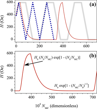
Figure 2. (a) An example of magnetic pulses of amplitude H0 = 600 Oe. The thick solid gray line depicts the trapezoidal pulses, the dotted dark-blue line—the triangular ones, and the thin solid red line is for the exponential pulses. (b) The shape of a single exponential pulse and the analytical expressions for its rising and trailing edges.
Download figure:
Standard image High-resolution imageThe triangular pulses consisted of alternating linear branches of increasing and decreasing magnetic field—from 0 to H0 and back [figure 2(a)]. The trapezoidal pulses had the same linear branches, only separated by horizontal lines of constant field (H = H0 and H = 0). The shape of each exponential pulse was determined by a piecewise-smooth function:

Here t = NMC/N0, NMC is the calculation time in Monte Carlo steps, and N0 is the time over which the magnetic field reaches maximum. The upper expression in (9) corresponds to the rising edge of the pulse and the lower one—to the trailing edge [as shown in figure 2(b)]. The exponent of 1.5 in the lower expression ensures the rise time is five times greater than the fall time. This shape of exponential pulses [only in the form of the upper expression in (9)] is often used in modern simulations [2]. However, in our case, the necessity to use a piecewise-smooth function is dictated by a significant increase in computational time. Had we used only the upper expression of (9), NMC would have been much greater than the characteristic relaxation time of the vortex system. Ultimately, the calculations would have taken much longer, but the result would have been almost the same (at least for the considered temperature).
The pulse rise time was fixed and identical for all three shapes (of equal amplitudes) and amounted to N0 ∼ 106 − 107 MC steps. The pulse amplitudes H0 took four different values from 600 to 1500 Oe (every 300 Oe). For the sake of convenience, the first pulse of each series started from H = Hc1 ≈ 391 Oe instead of rising from zero. Here Hc1 is the lower critical field at which the first vortex appears in the superconductor. Since all our samples were initially vortex-free, this did not influence the resulting data. Nonetheless, it allowed us to minimize the calculation errors and guarantee identical initial conditions (i.e., a fixed starting random number) for all three pulse shapes.
The samples under study contained various numbers of defects Ndef corresponding to low, medium, and high concentration ndef. The respective values of Ndef and ndef are shown in the first and second columns of table 1. Additionally, each number of defects could be distributed over the sample in two possible ways: a random scatter and a regular triangular lattice. The values of lattice spacing a for the latter type are presented in the third column of table 1. From here on, a sample containing the random scatter of defects shall be called sample ‛r' and the one with a triangular lattice—sample ‛t'. The average two-dimensional concentration ndef was roughly estimated as the total number of defects divided by sample area S = L2 = 25 μm2. When the defect distributions were generated, offsets of width ≈2λ were made on each side of the sample. This ensured the impossibility of creating vortices on defects in fields less than Hc1 (which would be physically incorrect).
Table 1. Characteristics of defect distributions.
| No. of defects | Averaged 2D concentration | Spacing of triangular |
|---|---|---|
| Ndef | ndef, 109 (cm−2) | latticea, (nm) |
| 165 | 0.7 (low) | 400 |
| 494 | 2.0 (medium) | 230 |
| 999 | 4.0 (high) | 160 |
3. Results
Figure 3 shows the calculated dependences of the averaged magnetic field induction Baverage on the calculation time NMC for various samples. Further on, these kinds of dependences shall also be called the ‛magnetic responses' of samples or simply ‛time dependences'. The curves in figure 3 are the results of the impact of three consecutive triangular (a), trapezoidal (b), and exponential (c) pulses of amplitude 1500 Oe. Here and on any such figure further on, the thick gray line demonstrates the magnetic pulse, the colored solid lines depict the responses of samples ‛r', and the dashed or dotted lines are for samples ‛t'. Baverage was determined as the total magnetic flux NΦ0 divided by the sample area S (thus, it had the meaning of magnetic flux density inside the sample).

Figure 3. Time dependences of the magnetic field inside samples with various numbers of defects (165, 494, and 999). Each sub-figure corresponds to pulses of different shapes: triangular (a), trapezoidal (b), and exponential (c). The pulse amplitude H0 = 1500 Oe. Two defect distributions were considered: a random scatter (r) and a triangular lattice (t).
Download figure:
Standard image High-resolution imageThe figures show that identical samples trap approximately the same field under pulses of different shapes. Moreover, the trapped field stays almost constant with the consecutive action of pulses within a series. The peak values of Baverage are very close for different samples and amount to ≈1250 Oe. However, unlike for other samples, the time dependences marked ‛999 t' (the pink dash-dot line in figure 3) strongly deviate from their respective pulse shapes.
Let us consider the magnetic responses of various samples to an exponential pulse in more detail. Figure 4 shows a scaled part of the time dependences from figure 3(c) demonstrating the first pulse and a half of the second one. To save space, we added an axis break in the interval NMC = (400 − 800) ⋅ 104, in which Baverage was almost constant. Some samples demonstrate a peculiar response to the first rising edge of the pulse. For the low defect concentrations, the time dependences have virtually the same shape as that of the pulse (curves ‛165 r' and ‛165 t'), whereas the samples with medium and particularly with high defect density behave differently. One may say that the ‛494 t', ‛999 r', and ‛999 t' curves have two nominal parts connected by a jump-like transition. The first part deviates from the pulse shape (it is bent toward the horizontal axis), and the second part does not. The transition between these parts is rather acute for the samples with triangular lattices of defects, while for the ‛r'-samples, it is much smoother. By the time the external field reaches its peak, the values of Baverage are approximately equal for samples with medium and low defect concentrations, whereas the ones with 999 defects show slightly smaller fields (figure 4).

Figure 4. Magnetic responses of samples with various defect concentrations to the first front edge, first trailing edge, and the second front edge of an exponential pulse of magnitude 1500 Oe (as in Figure 3). The black arrow points at small peculiarities of samples ‛494 r' and ‛494 t'. The paired red arrows denote similar features for curves ‛999 r' and ‛999 t'.
Download figure:
Standard image High-resolution imageNext, as the external field decays, Btrapped decreases rather quickly (within the first (1 − 2) ⋅ 106 MC steps). After that, Baverage relaxes slowly and negligibly for the rest of the trailing edge of the pulse. In the cases of 165 and 494 defects, the initial part of the negative slope of Baverage (before it reaches a constant value) follows the pulse shape. Moreover, the decrease in the magnetic induction of samples with high defect density occurs much slower. The residual trapped fields also vary. For instance, the type of defect distribution does not seem to influence the trapped field for the low and medium concentrations, while in the case of 999 defects, sample ‛t' demonstrates a higher result than that of sample ‛r'.
As can be seen from the second rising edge of the pulse in figure 4, Baverage keeps constant while the external field increases from zero to ≈500 Oe, after which all six samples begin to magnetize simultaneously. Then, as the pulse rises, the field inside the samples with moderate and high defect concentrations increases according to the pulse shape (except for a small part in the very beginning of the rising edge of curves ‛494 r' and ‛494 t', marked by a black arrow in figure 4). Once again, the samples with high defect concentrations deviate from the pulse shape. This time, however, the transition between the two parts is not jump-like and has a lower magnitude (as denoted by two red arrows in figure 4). The responses to further sections of the pulse behaved similarly.
Let us analyze the instant vortex distributions of the two samples with high defect density, obtained at various time points of their response to exponential pulses. Figure 5 shows the same scaled part of the exponential series as in figure 4, but only for the two mentioned samples (a solid line for ‛r' and a dash-dot line for ‛t'). Here, the arrows indicate the chosen time points, the integers in brackets denote their numbers (1–6), and the letters indicate the type of defect distribution. The vortex configurations corresponding to each time point are shown in figure 6: the column on the left is for sample ‛r', and the column on the right is for sample ‛t'. The central column shows the averaged distribution profiles of the magnetic field inside both samples. The colors and line styles are kept from the previous figure. Such profiles are often measured in experiments using Hall magnetometry [1–4, 10, 23, 57, 58]. In this paper, the magnetic profiles were calculated using the expression for the magnetic field of a solitary vortex (5). For simplicity, the sample was divided into square cells of size 2 nm ≪ λ, and in each cell, the contribution from all N vortices was summed. Then the resulting mesh was averaged along the y-axis.

Figure 5. Magnetic responses of samples containing 999 defects (as in figure 4) with labeled time points, in which instant vortex distributions were obtained.
Download figure:
Standard image High-resolution image
Figure 6. Instant vortex distributions of samples with high defect density (‛r' on the left and ‛t' on the right) at various time points (1–6) of an exponential pulse. Blue circles indicate the vortices, brown squares indicate the defects. The averaged distribution profiles of the trapped magnetic field Btrapped(x) over the sample width (in the center).
Download figure:
Standard image High-resolution imageIt can be seen right from the first pictures in figure 6 that the vortices begin to penetrate sample ‛r' sooner and much more quickly than sample ‛t' (containing exactly as many defects). The same number of vortices (corresponding to an internal field of ≈500 Oe) needs almost twice as much computational time to penetrate the sample with a triangular defect lattice than the one with a random scatter (subfigures (1.t) and (1.r) correspondingly). In the first case thereof, almost all vortices accumulate near the sample edges. For the random scatter, the vortices are distributed more uniformly, and about a quarter of them occupy the central part of the slab. This can be clearly illustrated on the magnetic profiles Btrapped(x) of both samples by comparing the heights of peaks on the edges or the depths of ‛valleys' in the central parts.
By the next time point, the magnetic profile of sample ‛r' has practically leveled out from the edges to the center, except for a slight inhomogeneity in the right central part of the profile. The latter was caused by a local blank space in the defect distribution, which can be seen in the bottom right part of subfigure (2.r). In sample ‛t', the vortices have begun to quickly fill the central part of the slab (2.t), and the valley of Btrapped(x) has begun to shrink (whereby the height of peaks on the sample edges barely changed). By the third time point (when the external magnetic field has reached its peak), both samples contain approximately the same number of vortices, and the magnetic profile has become almost flat.
Further on, as the external field goes down to zero, the free (unpinned) vortices gradually leave the sample. Those near the edges exit through the boundaries while those in the central part move toward the edges first and then exit the slab. The pinned vortices stay where they are and become the trapped magnetic flux. By time point 4, sample ‛r' contains both pinned and free vortices. This occurs because of the repulsive inter-vortex interaction: the unpinned vortices (those surrounded by occupied defects) become trapped and cannot leave the sample even when the external field is zero. Sample ‛t' also contains some free vortices remaining, and those are located in the geometric centers of triangles formed by three nearest occupied defects (4.t). The total trapped flux for this sample is slightly greater than for sample ‛r'. It should also be mentioned that at H = 0, the magnetic profile of ‛t' has an almost uniform dome shape, while the ‛r'-sample demonstrates a slight tilt to the left, also caused by the presence of local blank spaces in the right part of the slab [figure 6(4.r)].
Next, as the second pulse rises, the vortices begin to enter the samples again. By time point 5, the number of vortices in both slabs is equal, and their magnetic profiles have flattened out from edges to center. In sample ‛t', all the vortices have accumulated near the boundaries (5.t), whereas in sample ‛r', the flux has entered the blank spaces and compensated the tilt of the magnetic profile shown in (5.r). The sixth time point is a threshold for sample ‛t': the vortex density becomes critical on the edges [as can be seen from the sharp peaks near the sample borders in figure 6(6.t)] so that the slightest increase in the external field leads to the rapid diffusion of vortices into the sample center. After that, both samples behaved the same way as at time points 2–4.
4. Discussion
As mentioned above, the repetitive application of identical pulses of high amplitude does not increase the trapped field in our calculations. Judging by the vortex dynamics presented in figure 6, one may note that for H0 = 1500 Oe, all defects (and the spaces between them in samples ‛r') become occupied by vortices right after the first pulse. Therefore, it is impossible to pump the sample with any more vortices because the pinning potential has been exhausted. In many papers, the value of H at which the trapped field ceases to increase is called the saturation field [13, 14]. In our case, apparently, the pulse amplitude exceeds the saturation fields of all samples, including the ones with high defect concentration.
It is also worth mentioning that the results of PFM have shown no dependence on the pulse shape. In other words, the vortex system reacted to the external field in the same manner, whether H had changed linearly (triangular and trapezoidal pulses) or exponentially over time. This correlates with the results of our previous work [44], where we studied linear magnetization with various rise times (for the same temperature). This time, not only did the jump-like peculiarities (flux jumps) manifest similarly for all three pulse shapes, but they also occurred at the same critical (activation) magnetic fields. This could mean that the considered pulse rise times exceeded the characteristic relaxation times of the vortex system (for the given temperature). Therefore, the vortices adjusted to the alternating magnetic field almost instantaneously. All the aforesaid allows us to assume that our calculation results could differ for various pulse shapes only at much higher rise times. These, however, would presumably lie outside the range of applicability of the Monte Carlo method because the dynamic equilibrium would not be reached in such short times. Thus, it would be interesting to further study the magnetization processes in HTSs at higher temperatures used in real experiments.
Another feature of the vortex behavior is worth mentioning. Despite having different pinning distributions (which is due to the presence of clusters of defects and blank spaces), samples ‛999 t' and ‛999 r' showed approximately equal residual magnetization after pulses of 1500 Oe. Although there is an apparent difference in the trapped field of samples ‛r' and ‛t' in figure 5, one may conclude from figure 6(4.t) that this difference is determined only by the extra free vortices left in the center of sample ‛t'. Nevertheless, these vortices are energetically unstable because each can still move in the horizontal direction (along the rows of defects). As a result, if we leave this sample alone for some time, the free vortices will eventually reach the boundaries and exit the slab. Thus, the relaxation of trapped flux will occur.
For the random scatter of defects, the following picture is observed. As already mentioned, sample ‛r' contains local blank spaces (empty areas among defects). Eventually, some vortices become pinned on the defects surrounding these areas ane vortices inside (due to the repulsive nature of Uvort). However, if the force exerted on a free vortex by the magnetic field exceeds the repulsive interaction of this vortex with its pinned neighbors, the vortex will be able to enter the blank space. Then, as the magnetic field goes down to zero, the vortex stays trapped inside that area and does not leave the sample.
In the light of the above said, we may assume that once the unpinned flux relaxes in sample ‛t', the number N of vortices in both ‛t' and ‛r' samples will become almost identical. This speculation suggests that at least when analyzing samples with a triangular lattice and a random scatter of defects (and provided that both are fully magnetized—namely, the external field exceeds the saturation fields of both samples), the former is preferable. However, the advantage lies only in the trapped field quality, specifically, its distribution uniformity. From a quantitative point of view, both samples are equivalent. On the other hand, if the pulse amplitude does not reach the saturation field (or rather the activation field for sample ‛t'), the random scatter of defects may provide better quantitative flux trapping. The aforesaid motivates us to continue numerical simulations and consider other ways of distributing defects over the sample, namely those that may hinder the relaxation of free vortices.
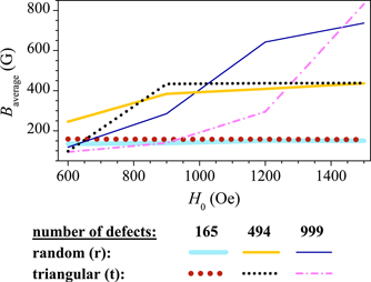
Based on the calculation results, the trapped field dependences on the pulse amplitude have been plotted. Figure 7 presents such dependences for samples with various defect concentrations. We shall once again point out that at the temperature considered in this paper, the pulse shape did not influence the amount of trapped flux for a given H0. Because of this, the plot presented in figure 7 was almost the same as for the other two pulse shapes. As shown in the figure, the field trapped by sample ‛165 t' almost does not change with H0. The reason is that even the amplitude of 600 Oe exceeds the saturation field for this sample. A random scatter of the same number of defects provides a slightly (within ∼10 − 15 vortices) smaller flux trapping efficiency at low amplitudes (600 − 900 Oe). However, the dependence saturates with the increasing amplitude and finally coincides with the horizontal dotted red line of sample ‛t' at H0 = 1500 Oe.
Figure 7. Dependences of the trapped field on the amplitude of exponential pulses for samples with various numbers and distributions of defects.
Download figure:
Standard image High-resolution image
In the case of sample ‛165 t', the defects are spaced at a rather large distance from one another (a = 400 nm ≈ 2λ). Therefore, the unpinned vortices can easily leave the sample when the external field goes down to zero. Thus, at the end of each pulse, the sample always contains the same number of vortices (equal to the number of defects). On the other hand, the number of vortices inside sample ‛165 r' continues to rise with the increasing amplitude even after the ‛165 t' line has saturated. This means that the saturation field of this sample is higher than that of the other. However, most of its flux trapping potential has already been exhausted at low amplitudes, so the increase in Baverage is not significant.
The samples with high and medium defect concentrations demonstrate growing Baverage(H0) dependences, and they also saturate at higher pulse amplitudes. For the case of 494 defects, sample ‛t' saturates at ≈900 Oe and sample ‛r'—only at ≈1500 Oe. The difference in the saturation fields for these two samples is more prominent than in the previous case. Similar dependences are observed for the samples with high defect concentration. However, we have not reached their saturation fields within the considered range of pulse amplitudes. Nevertheless, by mentally extrapolating these dependences onto higher pulse amplitudes, one may assume that their behavior will be analogous to the previous two samples.
5. Conclusion
In the present work, numerical modeling of the vortex system in a two-dimensional layered HTS with various defect concentrations and distributions has been conducted. The impact of magnetic pulses has been studied for three different pulse shapes. The main results of the study are the following:
- (a)At the considered temperature and pulse rise time, the height and shape of the trapped field distribution profile did not depend on the pulse shape. The vortex system adjusted to the alternating external field rather quickly (within ∼105 steps, which is significantly less than the pulse rise time), resulting in almost identical magnetization behavior for all three pulse shapes. The activation fields at which the flux jumps occurred were also the same for different pulses and depended only on the pinning distribution. Moreover, the consecutive application of three pulses of amplitude 1500 Oe did not lead to an increase in the trapped field, compared to the result for just one pulse. The pulse amplitude exceeded the saturation fields for all considered samples.
- (b)The saturation field rises with the increasing defect concentration because of the accumulation of vortex density near the sample edges and the emergence of a potential barrier. Samples with randomly scattered defects (‛r') demonstrated higher saturation fields than those with triangular defect lattices (‛t'). However, pulses of lower amplitude (600 − 900 Oe) magnetized the samples with random pinning more effectively. The near-edge potential barrier for these samples was less uniform, which allowed more vortices to penetrate the HTS.
- (c)Samples with random and periodic pinning (containing equal defect concentrations) trap almost the same amounts of flux if the pulse amplitude exceeds the saturation field of sample ‛t'. The difference between them displays only in the uniformity of the trapped field distribution inside the sample.
- (d)Great interest for further calculations lies in considering other temperature regimes and types of defect distribution. Doing this will allow us to study the vortex dynamics under pulsed magnetization in more detail and find the optimal pulse parameters.
Data availability statement
The data that support the findings of this study are available upon reasonable request from the authors.
Acknowledgments
The reported study was funded by RFBR, Projects No. 19-32-90279 (A N Moroz) and 17-29-10024 (A N Maksimova and I A Rudnev), and by RFBR and ROSATOM according to the research Project No. 20-21-00085 (V A Kashurnikov). The authors are grateful to the Ministry of Science and Higher Education of the Russian Federation (state assignment Project No. 0723-2020-0036) for the possibility of performing high-speed calculations.