

Abstract
The probability of the inter-Coulombic electron capture (ICEC) is studied for nanowire-embedded quantum-dot pairs where electron capture in one dot leads to electron emission from the other. Previous studies pointed to an interdependence of several ICEC pathways which can enhance the ICEC reaction probability. To identify favorable criteria for such synergies in a qualitative and quantitative manner, we conducted a considerable amount of simulations scanning multiple geometrical parameters. The focus of the paper is not only to find the geometries which are most favorable to ICEC but most importantly to explain the basic principles of the ICEC probability. We have thus derived a number of energy relations among solely single-electron level energies that explain the mechanisms of the multiple reaction pathways. Among them are direct ICEC, both slowing or accelerating the outgoing electron, as well as resonance-enhanced ICEC which captures into a two-electron resonance state that decays thereafter. These pathways may apply simultaneously for just one single geometric configuration and contribute constructively leading to an enhancement of the reaction probability. Likewise some conditions are found that clearly turn down the ICEC probability to zero. The results based on single-electron relations are so general that they can as well be used to predict the ICEC probability from the electronic structure in arbitrary physical systems such as atoms or molecules.
Export citation and abstract BibTeX RIS
1. Introduction
In the last few decades, semiconductor quantum dots (QDs) have gained much attention among nanostructured solid-state materials. They became inherent to numerous technological applications as e.g. photodetectors [1, 2], lasers [3, 4], or LEDs [4, 5]. Quantum dots find further use in single-photon emitters [6–9], catalysts [10], solar cells [10–13], and other energy conversion applications [12, 14]. Last but not least, they might potentially come into application in electronic components for quantum information technology [15–17]. Their success emerges from the rather straightforward fabrication and control over shape and size. In turn, realized geometries sensitively determine the electronic structure and related properties of the QD [18–21].
Recently, also the fabrication of arrays of QDs has become vastly controllable. Information technology is predominantly driving these developments as two tunneling-decoupled QDs with two tunable and long-range coupled spins are envisioned as qubits [15]. In more closely placed QDs, so-called quantum dot molecules, tunneling of charge carriers is within reach and instrumentalized, for instance, to stabilize excitons via separation of electrons and holes [22, 23].
Several routes to procure such QD pairs are being followed. Colloidal QDs can be assembled with the aid of linker molecules [24]. Mere solid state synthesis is possible through self-assembly, where QDs can be arranged either vertically by stacking of layers [23, 25, 26] or laterally by a pre-etching procedure [27]. Moreover, QDs and embedding materials can be alternately grown into wires [28, 29] or can be defined electrostatically within a wire or a two-dimensional electron-gas structure [30].
Interactions of charge carriers on different QDs and their resulting processes depend sensitively on the inter-quantum dot distance. They vary from being tunneling-coupled via spin-coupled to Coulomb-coupled. The latter type of interaction, which is applicable to long-distance paired QDs, has not yet attracted much attention from an experimental viewpoint despite progress in theoretical studies [31–34].
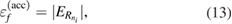
One recently discovered process is the inter-Coulombic decay (ICD), in which excitation energy is transferred from one electronically relaxing QD onto the neighboring QD, which is in turn ionized [31, 32]. This process appears also relevant in stacked quantum wells [34, 35]. Another process of interest here is the inter-Coulombic electron capture (ICEC) where an impinging electron is captured by one QD in accompaniment with the emission of another electron from the neighbor [33, 36]. A scheme of the ICEC processes is shown in figure 1(a).
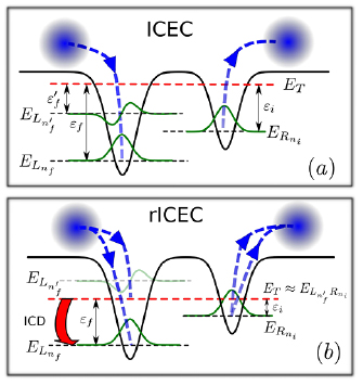
Figure 1. Scheme of (a) direct ICEC and (b) its combination with resonance-enhanced ICEC (rICEC). In ICEC the capture of the electron approaching from the left is accompanied by emission of the electron from the right quantum dot. The process is driven by electron correlation and the transferred energy ET is conserved. In the particular case of rICEC, a capture into a resonantly excited dielectronic state with energy  with one electron in the excited state of the left QD
  and one in the right dot
  happens. That resonance state can decay by emission of the right electron and simultaneous relaxation of the left electron to the ground state, a manifestation of ICD. The population of the resonance is not independent of the direct ICEC into the bound states located in the left QD which is indicated in figure (b). Both processes occur simultaneously.
Download figure:
Standard image High-resolution imageWithout loss of generality one may name the quantum dots left (L) and right (R) quantum dot and assume an incident electron (e) of energy  from the left. It is possible then to describe the ICEC process by the equation

where we used L and R to indicate the left and right localization of the paired-quantum-dot orbitals and ni and nf for the energy levels in each QD with i(f ) being the initially (finally) populated one. Moreover, in the case a dielectronic resonance state  is present with one electron in an excited level
  in the left QD in the system, it can be temporarily populated as

and electron emission will occur from this state through a following ICD. This resonance-enhanced ICEC (rICEC) is depicted in figure 1(b). We stress in the scheme that, even though rICEC seems to be an independent process, it is not, because of the correlation to the direct ICEC to  . In other words, we expect the dynamics of both channels to affect each other due to the emission at the same energy. Therefore, although very related to ICD, rICEC is expected to have a richer physical behavior.
Studies on ICD revealed that the inter-dot distance is not the only influential variable to inter-quantum dot energy transfer processes. Geometry variations of the individual QDs foster changes of the electronic structure (known as the quantum-size effect [18–20]) which, in turn, alter ICD. This was systematically analyzed taking into account the non-trivial interdependence of several geometric parameters [37–39]. First hints on how geometry changes also ICEC have already been collected in computations on nanowire-embedded paired n-doped QDs [33, 36, 40].
Those recent computations on QDs have proven in accord with the first predictions for atomic systems [41, 42] that ICEC is far more intricate than ICD. Firstly, free-electron states occur as both initial and final states. Secondly, ICEC was shown to be energy selective [33, 36], a feature that had been overlooked in the first scattering calculations on pairs of atoms or molecules [41, 42]. And thirdly, its efficiency can be extraordinarily increased if the ICEC peak energy matches the two-electron resonance corresponding to an ICD process (rICEC, see figure 1(b)) for which we can recently offer a more detailed understanding of the necessary conditions [40]. A comprehensive analysis on this multitude of requirements on the electronic structure and a systematic understanding of the process's dependence on them are still missing.
To this end, we employ again highly-accurate electron dynamics calculations in general binding potentials in which we scan over a multitude of 8613 QD pair geometries. This extensive scan itself is possible for two reasons. On the one hand, we have found for both, the ICD and the ICEC process that although the system is three-dimensional, calculations in a one-dimensional model are largely valid because the continuum spans in one dimension only and an accurate approximation to the Coulomb operator was found [36, 40, 43]. On the other hand, we have made numerous technical improvements to fit the Coulomb potential as well as other parameters in the calculations which has led to a significant speedup of calculations [37].
For each of the scanned configurations, we calculate the maximum of the ICEC reaction probability (a measure of the amount of electron emission, discussed further in section 3) and recognize regions of ICEC enhancement or quenching. One strict energy requirement determining whether ICEC can occur had already been found with a resonance pathway enhancing ICEC (figure 1(b)) [33]. As we will see here, the conjunction of two or more conditions that enhance the reaction probability (RP) is synergistic and amplifies the probability. Moreover, a higher efficiency of ICEC compared to that of competing energy release pathways, namely photo recombination [31] and phonon emission [44] was found to be valid in the systems under investigation.
We start our presentation in section 2 by describing the paired-quantum dot model, the numerical approach used in the calculations, and the definition of the computed quantities. In section 3, we lay out the theory of the direct (section 3.1) and resonance-enhanced (section 3.2) ICEC process, from which we deduce different relations between single-electron energies which will help to decipher the scanned electron dynamics reaction probability results. For clarity, these relations are summarized in section 3.3, which is followed by the computational details (section 4).The results for multiple inter-depending geometrical parameter variations are presented in section 5 where we test how the different ICEC pathways contribute to the RP before we conclude (section 6).
2. The model
In this work, we focus on nanowires with embedded QD pairs. One experimental implementation of the device places a nanowire on top of a grid of metallic gates which can then be used to localize the conduction band electrons through the electrostatic potential [30, 45]. Implementations with layered semiconductors where also intensively tested experimentally [23, 25, 26, 28, 29] for which it is possible to perform the same calculations as presented here. For the theoretical description we use a binding potential model presented in detail in [36] to describe the electrons in the conduction band of the semiconductor.
The Hamiltonian term imposed by the nanowire and quantum-dot pair acting on each electron is
This represents a one-electron Hamiltonian in which

are the transverse confinement by the wire and the longitudinal open potentials from the embedded QDs, where m* is the effective mass, R is the distance between centers of the QDs and bL,R parameterize the sizes of the left and right QD while  express their potential depths [33, 36].
The two-electron effective-mass Hamiltonian for the system is
where  is the relative dielectric permittivity,
 ![$ \newcommand{\ve}[1]{\mathbf{#1}} \ve{r}_1$](https://content.cld.iop.org/journals/0953-8984/32/6/065302/revision2/cmab41a9ieqn010.gif) and
and ![$ \newcommand{\ve}[1]{\mathbf{#1}} \ve{r}_2$](https://content.cld.iop.org/journals/0953-8984/32/6/065302/revision2/cmab41a9ieqn011.gif) are the respective electron position vectors in atomic units of electron rest mass
are the respective electron position vectors in atomic units of electron rest mass  , elementary charge
  , reduced Planck constant
  , and Coulomb constant
 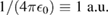 In these units, the effective Bohr radius is
  below which strong quantization is expected. We adapt the atomic unit system to incorporate the effective mass m* and the relative permittivity
  which simplifies the formulae. Realistic quantum dot parameters for a specific semiconductor of choice are connected to the Hamiltonian parameters by the scaling
 ![$ \newcommand{\ve}[1]{\mathbf{#1}} \newcommand{\e}{{\rm e}} \ve{r}_i \to \frac{\epsilon_r}{m^*}\ve{r}_i$](https://content.cld.iop.org/journals/0953-8984/32/6/065302/revision2/cmab41a9ieqn018.gif) of the electronic coordinates [36]. These effective atomic units are used throughout and noted
of the electronic coordinates [36]. These effective atomic units are used throughout and noted  as well.
In the strong transversal confinement regime (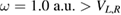 ), three-dimensional simulations are very well represented using an effective one-dimensional model [46] obtained using the wave-function separation ansatz

where  is the two-dimensional single-electron ground state function transverse to the nanowire and
  is the longitudinal effective wave function. This approach has been successful in the description of bound and resonance states in nanowires [36] and semiconductors in an external magnetic field [47]. We choose the triplet state such that
  , and hence
 ![$ \newcommand{\ve}[1]{\mathbf{#1}} \Psi(\ve{r}_1, \ve{r}_2)$](https://content.cld.iop.org/journals/0953-8984/32/6/065302/revision2/cmab41a9ieqn024.gif) , are antisymmetric under exchange of electrons. The effective one-dimensional Hamiltonian has been deduced from the analysis of the expectation value of the full Hamiltonian according to [36] as
, are antisymmetric under exchange of electrons. The effective one-dimensional Hamiltonian has been deduced from the analysis of the expectation value of the full Hamiltonian according to [36] as
and  such that the distance z12 between the electrons is scaled by the characteristic transverse confinement length
 ![$ \newcommand{\bra}[1]{\left\langle #1 \right|} \newcommand{\braket}[3]{\left\langle #1 \left| #2 \right| #3 \right\rangle} l=\sqrt{\braket{\phi_0}{x^2}{\phi_0}}=1/\sqrt{\omega}$](https://content.cld.iop.org/journals/0953-8984/32/6/065302/revision2/cmab41a9ieqn026.gif) , and '
, and ' ' denotes the error function. The asymptotic behavior of the effective potential exhibits the correct 1/z12 dependence at large electron separation, but it does not, however, diverge at infinitely small distances between the electrons where
  .
.
Since we consider the center-to-center distance R between the QDs just big enough to have the eigenstates well localized in the left or right dot and further assume different potential depths  , the electronic level structure obtained from the longitudinal potential
  can be labeled by Ln and Rn, in the left or right quantum dot respectively with
  and eigenenergy
  . The symmetry is fairly close to that of levels in a box potential: L0 corresponds to a nodeless symmetric state around the left dot center, L1 to an antisymmetric state with one node in the left dot center, and so on. Once there are no further energy levels accommodated in the QDs, the orbitals of the succeeding levels spread over the entire space as continuum states of free electrons denoted with
  .
.
3. Energy relations for ICEC processes
In this section we describe the ICEC and rICEC processes for our QD pair model of section 2. We introduce the basic quantities used to assess the processes' effectiveness and, through physical considerations, we derive the constraints and conditions for single-electron energies that define regions of particularly high or low ICEC probability.
3.1. Direct ICEC
The basic set of equations for energy conservation for ICEC in quantum dots are,


As reflected by figure 1,  and
and  are incoming and outgoing electron energies, ET is the total energy and
  and
and  are the initial and final energies of the QD pair system, i.e. the single-electron bound state energy for the initial and final state. The one-electron threshold energy in our model is set to zero, so the bound state energies are all negative. From equations (10) and (11) we see that the outgoing electron energy
  can be greater or smaller than
  of the incoming electron. Moreover, the ICEC channel can be closed due to energy constraints which require the incoming electron to fulfill the energy conditions


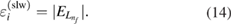
Let us analyze the energy transfer between the QD pair and the free electron for either case of equation (12):
- (a)In the case that
 the QD pair releases excess energy to the outgoing electron which is then faster than the incoming one (accelerating configuration, see figure 2(a)),
 - (b)In the opposite case,, the QD pair absorbs energy from the incoming electron and the outgoing electron turns out to be slower (slowing configuration, see figure 2(b)).


Figure 2. ICEC schemes showing the configurations of the accelerating (a) and slowing (b) process for which the maximum of the reaction probability is obtained through matching of energy differences  with level energies according to equation (17). Note that in the case of accelerating ICEC the final state is the ground state
  , in case of slowing ICEC an excited state
  and we assume that other existing levels do not play a role for the energy location of the reaction probability maximum.
Download figure:
Standard image High-resolution imageIn previous works it was shown for the accelerating configuration that the direct ICEC process gives a peak in the energy-dependent RP at a given incoming electron energy [33, 36]; the underlying flux profile has a Gaussian shape [40]. Hence, in case of accelerating ICEC, the reaction probability peak position is where the outgoing electron takes exactly all the energy initially contained in the QD pair, i.e.  . The respective condition
was also found in [36]. Owing to this interpretation, it is straightforward to perform the same analysis for the case of the slowing ICEC process, which was not previously addressed. Accordingly, the peak of the reaction probability as function of the incident electron energy is to be found where the incoming electron energy  can be completely absorbed by the QD pair in its final state
  , thus
Using equations (13) and (14) in equations (10) and (11), respectively, one can obtain the initial energy for the accelerating case and the final energy for the slowing case,


These two results can be used to compute the value of the total energy for the configuration at which the peak in the RP is found. For the two cases of ICEC processes, accelerating and slowing, the total energy turns out to have the same expression

In any case, the incoming and final electron energies need to be positive for ICEC to be open. We consequently arrive at the following equations for the binding energies


3.2. Resonance-enhanced ICEC
The reaction probability obtained for direct ICEC has been found to be very small and barely reaching  at peak values [33, 36]. This can render ICEC being impossible to observe, even when it is an ultrafast process happening in times estimated around 10 ps in GaAs. However, the presence of two-electron resonance states has shown to give an extraordinary reaction probability enhancement when energy suffices to populate them [33, 36]. We call this process a resonance-enhanced ICEC, or rICEC.
In our current system shown in figure 1(a), the left dot binds besides  an additional
  level. Potentially, the two-electron resonance
 ![$ \newcommand{\bi}{\boldsymbol} \newcommand{\ket}[1]{\bigl| #1 \bigr\rangle} \ket{L_{n^\prime_{f}}R_{n_{i}}}$](https://content.cld.iop.org/journals/0953-8984/32/6/065302/revision2/cmab41a9ieqn051.gif) can be populated, as shown in figure 1(b). Its decay time and energy were computed in many cases when describing ICD in quantum dots [31, 37] along the path
can be populated, as shown in figure 1(b). Its decay time and energy were computed in many cases when describing ICD in quantum dots [31, 37] along the path

We are going to approximate the resonance energy at large distances R by
throughout this study. This implies that we calculate it solely from single-electron energies which are easy to access in a potential device. The validity of this approximation is discussed in detail in [40]. To ensure the decay ![$ \newcommand{\bi}{\boldsymbol} \newcommand{\ket}[1]{\bigl| #1 \bigr\rangle} \ket{L_{n^\prime_f}}\longrightarrow\ket{L_{n_f}}$](https://content.cld.iop.org/journals/0953-8984/32/6/065302/revision2/cmab41a9ieqn052.gif) in the left quantum dot allows for ionization
in the left quantum dot allows for ionization ![$ \newcommand{\bi}{\boldsymbol} \newcommand{\ket}[1]{\bigl| #1 \bigr\rangle} \ket{R_{n_i}} \longrightarrow e^-(\varepsilon_f)$](https://content.cld.iop.org/journals/0953-8984/32/6/065302/revision2/cmab41a9ieqn053.gif) of the right electron, the energetic constraint
of the right electron, the energetic constraint

has to be met. Upon electron capture as in ICEC, the energy of the resonance state  can in principle be above or below the initial QD pair energy
  , but since
  (see equation (10)) the resonance state can only be populated if it is above. Hence the condition that the resonance must fulfill, derives as
Once this condition is met, it may be possible to match the direct ICEC peak condition of  and the resonance energy
  , to render a huge enhancement of the reaction probability at resonance energy. Direct ICEC can occur to any
 ![$ \newcommand{\bi}{\boldsymbol} \newcommand{\ket}[1]{\bigl| #1 \bigr\rangle} \ket{L_{n_{f}}}$](https://content.cld.iop.org/journals/0953-8984/32/6/065302/revision2/cmab41a9ieqn059.gif) state for which the condition of equation (12) is fulfilled. Different final states change the total energy, and hence to observe rICEC, the resonance energy must match one of the total energies defined by equation (17) at which the reaction probability has a peak. We write this condition as,
state for which the condition of equation (12) is fulfilled. Different final states change the total energy, and hence to observe rICEC, the resonance energy must match one of the total energies defined by equation (17) at which the reaction probability has a peak. We write this condition as,

where we assume the direct ICEC can be related to a bound state ![$ \newcommand{\bi}{\boldsymbol} \newcommand{\ket}[1]{\bigl| #1 \bigr\rangle} \ket{L_{n_{f}}}$](https://content.cld.iop.org/journals/0953-8984/32/6/065302/revision2/cmab41a9ieqn060.gif) that is different from the one forming the resonance state, in this case
that is different from the one forming the resonance state, in this case ![$ \newcommand{\bi}{\boldsymbol} \newcommand{\ket}[1]{\bigl| #1 \bigr\rangle} \ket{L_{n^\prime_{f}}}$](https://content.cld.iop.org/journals/0953-8984/32/6/065302/revision2/cmab41a9ieqn061.gif) .
.
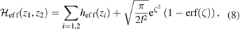
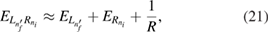
The schemes in figure 3 display two examples for electronic level and state configurations which may occur upon changing the geometry. In both panels the energy of the resonance,  , is shown as a green dashed line. The slowing ICEC related quantities are depicted in red and those corresponding to accelerating ICEC in blue. The PR peak conditions,
  and
and  (see equation (17)), are fulfilled in both panels. In panel (a) the resonance state energy is not matching any of the total ICEC energies
  and
and  and hence equation (25) is not fulfilled. Conversely, in panel (b), both slowing and accelerating ICEC energies match that of the resonance (i.e. for the resonance with
  and ni = 0, equation (25) is fulfilled for both final states nf = 0 and nf = 1), showing the coalescence of three processes at one single energy.
Figure 3. Schematic representation of the quantum dot pair with different level arrangements (note that for simplicity we did not change the shape of the QDs accordingly). In both panels, condition a maximum of the slowing ICEC peak,  , is fulfilled and is represented by red lines and arrows (see equation (17)). Condition
  for the accelerating ICEC peak is also fulfilled and is shown in blue. In (a) conditions 3 and 4 are not fulfilled because
  (green dash-dotted), and condition 5 (
 ) also fails. In (b) all three conditions are fulfilled; for clarity reasons we only slightly shifted the three energies.
Download figure:
Standard image High-resolution image3.3. Summary of relevant energy relations
The maximum of the reaction probability is strongly dependent on the geometry of the QD pair. In sections 3.1 and 3.2 we derived relations between the one-electron energies and the approximated resonance energy that define areas in the parameter space  with zero or very high maximum RP. These relations are implicit equations that define curves in the two-dimensional parameter space. We will show that some of them follow the maximum peak. Others define boundaries that divide the plane in regions where the respective condition is fulfilled or not. In the relations we assume
  .
.
- 1.The autoionizing resonance state is labelled after the one-electron states and . The condition ensures that the energy level is below the single-electron threshold energy E = 0.
- 2.The resonance can only be populated if it is above the initial energy .
- 3.Here we match the total energy as obtained for the ICEC peak to (equation (17)) to the resonance energy. This means that both the slowing ICEC to and rICEC coincide.
- 4.
- 5.Coincidence of direct ICEC into (slowing) and (accelerating). This condition can be used to detect an increase or decrease (interference) of the reaction probability due to a contribution from two different ICEC processes.
- 6.The crossing of and . This is relevant since it changes the direct ICEC to the state from slowing to accelerating. It also helps to understand the behavior of the lines defined by other conditions that also involve these two energies. Note that the energies do not cross in the actual spectrum (they show an avoided crossing), what changes is the ordering of the states.
- 7.The crossing of and . This is relevant since it changes the direct ICEC to the state from accelerating to slowing.
- 8.Condition 6 points to the crossing of and . This affects the behavior of the curves defined by condition 4, and the present condition helps to understand such behavior.

![$ \newcommand{\bi}{\boldsymbol} \newcommand{\ket}[1]{\bigl| #1 \bigr\rangle} \ket{L_{n^\prime_{f}}R_{n_i}}$](https://content.cld.iop.org/journals/0953-8984/32/6/065302/revision2/cmab41a9ieqn075.gif)


4. Computational details
We have performed numerical calculations of the dynamics of ICEC for various QD distances R, potential depth  and size parameters bL for the left quantum dot using the two-electron effective Hamiltonian represented by equation (8) and determined how the geometric parameters influence the ICEC probability. The radius of the wire was fixed in all the calculations by the transverse confinement length set to
  The quantum-dot center-to-center-distance was varied between
  and
and  , the potential depth of the left QD between
  and
and  , and its size parameter between
  and
and  as summarized in table 1 together with all computational parameters. This parameter region includes configurations with one or two bound states within the left dot and configurations where the left dot is deeper or shallower than the right one.
The numerical calculations where performed using the MCTDH algorithm [48, 49] as implemented in the MCTDH Heidelberg package [50, 51]. The underlying basis in discrete variable representation (DVR) is a Sine-DVR grid expanding over 431 points and ranging from  to
to  in the z direction which allows for an accurate representation of the continuum electron.
The one-electron states of the QDs and their energies  were obtained from the exact diagonalization of the effective Hamiltonian
  according to equation (9). When turning to two-electron states, the full Hamiltonian
  applies. It includes the Coulomb interaction potential which is brought into a sum-of-product (Tucker) form as required by MCTDH using the Potfit algorithm including all possible terms such that a full representation of the potential in the primitive basis is achieved [50, 52, 53]. Furthermore, a total of 14 SPFs for the two modes, i.e. the coordinates of the electrons, sufficed to retain orbital occupations below about 10−6 for the highest-energy orbital.
In all two-electron dynamics calculations, we have used the same initial wave function, i.e. incoming wave packet and initial state. One electron is always initially bound in ![$ \newcommand{\bi}{\boldsymbol} \newcommand{\ket}[1]{\bigl| #1 \bigr\rangle} \ket{R_{n_{i}}} = \ket{R_0}$](https://content.cld.iop.org/journals/0953-8984/32/6/065302/revision2/cmab41a9ieqn115.gif) with the right QD kept constant having parameters
with the right QD kept constant having parameters  for the size and
  for the potential strength. The wave packet is described by a Gaussian wave initially centered at
  with group momentum
  and a width
  The initial energy is
  and its energy width
  We based this choice on the fact that we know the reaction probability can be computed in an energy range as wide as the energy distribution of the incoming wave packet. The RP needed to asses the emission of electrons coming from an ICEC process is defined as the percentage of electron emission from the state with energy
  that is correlated with the other electron having a specific energy distribution undergoing capture into the state with energy
  as exactly defined in [36, 40, 50]. For its computation absorbing boundary conditions are mandatory and were implemented through complex absorbing potentials (CAPs) [54] of quadratic order located outside the reaction region at
  The strength of the CAPs was tuned to
  in order to obtain a minimal value of the reflection and transmission coefficients for the given CAP parameters together with the energy range of the system, as can be seen in table 1.
Table 1. Choice and range of computational parameters.
| Electron parameters | ||
|---|---|---|
 |
 |
 |
| Quantum-dot-pair parameters | ||
![$ \newcommand{\au}{{\;\mathrm{a.u.}}} b_L \in [0.09\au,\; \ldots,\; 0.60\au]$](https://content.cld.iop.org/journals/0953-8984/32/6/065302/revision2/cmab41a9ieqn130.gif) |
 |
|
![$ \newcommand{\au}{{\;\mathrm{a.u.}}} V_L \in [0.40\au,\;\ldots,\;1.10\au]$](https://content.cld.iop.org/journals/0953-8984/32/6/065302/revision2/cmab41a9ieqn132.gif) |
 |
|
![$ \newcommand{\au}{{\;\mathrm{a.u.}}} R \in [6.00\au,\; \ldots,\; 12.0 \au]$](https://content.cld.iop.org/journals/0953-8984/32/6/065302/revision2/cmab41a9ieqn134.gif) |
 |
|
| DVR type | z range | Grid points |
| sin |  |
431 |
| SPF configurations |  , id , id |
|
CAP  |
 |
 |
 |
 |
 |
 |
 |
 |
5. Results
For simplicity and easier understanding, we summarize the energy conditions derived in section 3.3 using the states that we considered in our calculations. Namely,  is always the ground state of the left quantum dot L0,
  the first excited state of the left QD L1, and
  the ground state of the right QD R0. The energy relations of section 3.3 specified for this system are thus summarized in table 2 together with their line types.
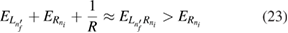
Table 2. List of the conditions parametrizing the curves in figures 4–6 used to explain the areas of differently high reaction probability. The energies of the levels are functions of the geometrical parameters  .
.
| Condition | Line type | Expression |
|---|---|---|
| 1. Second level in left quantum dot | White, dash-dotted |  |
| 2. Two-electron resonance above initial threshold | Red, dash-dotted |  |
| 3. Coincidence of slowing ICEC and rICEC | Yellow, solid |  |
| 4. Coincidence of accelerating ICEC and rICEC | Cyan, solid |  |
| 5. Coincidence of direct ICEC to L1 (slw) and L0 (acc) | Dark blue, solid |  |
6. Crossing of  and and  |
Light blue, dashed |  |
7. Crossing of  and and  |
Green, dashed |  |
| 8. Coincidence of resonance with L1-L0 energy gap | Magenta, solid |  |
Electron dynamics was used to calculate the ICEC process for 8613 different configurations of QD pair geometries to deduce the geometry dependence, or the quantum-size effect, of the ICEC RP. The size parameter bL and potential depth  of the left dot were varied for different inter-dot separations R. For each configuration the maximum of the RP was computed resulting in the color maps of figures 4 and 6. All plots show a more or less pronounced Y shape of highest reaction probability in orange-red colors that lies diagonally in the color maps as well as surrounding zero-probability areas in black. From such common features we can assume certain conditions for ICEC to function in a favorable way or not. In sections 3.1 and 3.2 we have already introduced the different flavors of ICEC, a slowing and an acceleration direct process as well as a resonance-enhanced one that will eventually coincide under certain energetic conditions and make ICEC extremely probable. The summary of the most directive conditions (section 3.3) will be used here to explain the maximum reaction probability shape as function of geometry, which will be done first for the
  case in the right panel of figure 4, before the trends for other R are discussed.

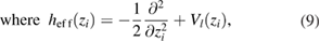
Figure 4. Reaction probability (RP) in % according to the color bar and contours ( and
and  ) as a function of the left dot size bL and depth
  . The panels are labelled with the distances
  between the two quantum dots. Note that the RP maxima follow closely the triple coincidence of conditions 3 (yellow), 4 (cyan) and 5 (blue) according to the interpretation provided in the text. The condition number and line types of the curves are given in table 2.
Download figure:
Standard image High-resolution imageAs was already found in previous works [33, 36, 40], the strongest RP enhancement occurs when, besides direct ICEC pathways, there is also an rICEC channel in which the resonance ![$ \newcommand{\bi}{\boldsymbol} \newcommand{\ket}[1]{\bigl| #1 \bigr\rangle} \ket{L_1R_0}$](https://content.cld.iop.org/journals/0953-8984/32/6/065302/revision2/cmab41a9ieqn173.gif) is available for population by the incoming electron and successive ICD. This is possible under two conditions. On the one side, the bound state
is available for population by the incoming electron and successive ICD. This is possible under two conditions. On the one side, the bound state ![$ \newcommand{\bi}{\boldsymbol} \newcommand{\ket}[1]{\bigl| #1 \bigr\rangle} \ket{L_1}$](https://content.cld.iop.org/journals/0953-8984/32/6/065302/revision2/cmab41a9ieqn174.gif) has to exist at all, i.e.
has to exist at all, i.e.  . This is bound by condition 1 which is shown in the color maps and in the diagram of figure 5 as a white dashed-dotted line. Geometrically, QDs that are either too shallow (small
  ) or too narrow (large bL) allow only for one bound level. On the other side, condition 2,
  , says that the resonance energy is not high enough to lead to ionization of the right QD. The region to the left of the red dashed-dotted line in figure 4 for
  (and in figure 5) shows that the geometries causing this behavior have a wide and deep left dot with a low-lying
 ![$ \newcommand{\bi}{\boldsymbol} \newcommand{\ket}[1]{\bigl| #1 \bigr\rangle} \ket{L_1}$](https://content.cld.iop.org/journals/0953-8984/32/6/065302/revision2/cmab41a9ieqn179.gif) state and thus also a low resonance energy
state and thus also a low resonance energy  .
.
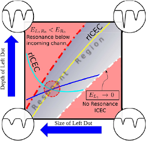
Figure 5. Diagram of the color-coded curves obtained from the energy conditions listed in table 2. The grey-shaded area is where the maximum reaction probability is expected because there is a resonance above the incoming threshold energy and rICEC is possible. The red dashed circle encloses the matching of conditions 3, 4 and 5. It is thereby the point where maximum RP is expected.
Download figure:
Standard image High-resolution imageAs a first conclusion one can classify three regions. Two for large and small left dots, respectively, where rICEC is energetically forbidden and one area for intermediate quantum dot sizes where it is allowed and the RP is largest. Those regions are summarized graphically in figure 5. Grey shows where rICEC occurs. In the lower red region rICEC is not possible because the resonance state ![$ \newcommand{\bi}{\boldsymbol} \newcommand{\ket}[1]{\bigl| #1 \bigr\rangle} \ket{L_1R_0}$](https://content.cld.iop.org/journals/0953-8984/32/6/065302/revision2/cmab41a9ieqn181.gif) does not exist. In the upper region it is below threshold.
does not exist. In the upper region it is below threshold.
Now we turn to discuss the structure of the reaction probability maxima observable within the rICEC region for the  case. Immediately it becomes evident that the main contribution to the RP follows the yellow solid line from the lower left to the upper right corner, that is from shallow wide to narrow deep left quantum dots all accommodating two energy levels L0 and L1. The line is drawn to visualize condition 3, which is
  in figures 4–6. Physically it means the coincidence of direct ICEC with capture into the
 ![$ \newcommand{\bi}{\boldsymbol} \newcommand{\ket}[1]{\bigl| #1 \bigr\rangle} \ket{L_1}$](https://content.cld.iop.org/journals/0953-8984/32/6/065302/revision2/cmab41a9ieqn184.gif) level slowing the outgoing electron (see figure 2(b)) and of the resonance-enhanced ICEC through electron capture into the resonance state
level slowing the outgoing electron (see figure 2(b)) and of the resonance-enhanced ICEC through electron capture into the resonance state ![$ \newcommand{\bi}{\boldsymbol} \newcommand{\ket}[1]{\bigl| #1 \bigr\rangle} \ket{L_1R_0}$](https://content.cld.iop.org/journals/0953-8984/32/6/065302/revision2/cmab41a9ieqn185.gif) . Mathematically it comes from the matching of the energy of the slowing ICEC peak (equation (17)) to the resonance energy
. Mathematically it comes from the matching of the energy of the slowing ICEC peak (equation (17)) to the resonance energy  .
.

Figure 6. Reaction probability (RP) in % according to the color bar and contours ( and
and  ) as a function of the left dot size bL and depth
  . The panels are labelled with the distances
  between the two quantum dots. Note that the RP maxima follow closely the triple coincidence of conditions 3 (yellow), 4 (cyan) and 5 (blue) according to the interpretation provided in the text. The condition number and line types of the curves are given in table 2.
Download figure:
Standard image High-resolution image
In the color maps (figures 4–6) condition 4 is drawn as a cyan solid line. It curves from large  with small bL, a configuration where even three levels may occur, to intermediate values for each parameter, finishing at
  and
and  for the case of
  , where the L1 level disappears (white dashed-dotted line).
In figure 4, it further becomes evident that there is a crossing of the implicit curves for both conditions 3 and 4 matching direct and resonance-enhanced ICEC. It occurs near the point where the reaction probability maximum gets its maximal value in the whole scanned 2D area. Conditions 3 and 4 will both be fulfilled whenever  , which is made a self-standing condition number 5 drawn as dark blue solid line diagonally ranging from low
  and bL values to large ones (however less steeply than the yellow line of condition 3). The triple-coalescence point of all conditions 3, 4 and 5 at the RP maximum, is highlighted in scheme of figure 5 with a red circle. The energetic matching is to be seen from figure 3(b).
Condition 5 is basically the energy difference between single-electron levels. Hence, any connection to the resonance energy is lifted and actually condition 5 can be fulfilled by direct ICEC only without resonance enhancement. It only signifies the coincidence of direct ICEC into the L0 state (accelerating case) and into the L1 state (slowing case). This becomes most apparent in the  panel of figure 4 in the region where there is no resonance, that means below the white dashed curve on the right side of the Y-shaped area of maximal reaction probability. The contribution to the RP here is small when compared to the rICEC cases on the left branch of the Y shape, which was to be expected from our previous findings [33, 36, 40].
There are two further conditions associated only with the direct ICEC pathways and these are condition 6 (light blue dashed lines) and 7 (green dashed lines). Both are equalities of single-electron levels energies,  and
and  , respectively. They apply when two levels, one located in the left and the other in the right QD, change their order. For the case of condition 6 this means that in deep and broad left QDs the energy of the L1 state drops under that of the R0 state and actually leads to a change of quality of the direct ICEC process from slowing to accelerating. Condition 7 applying to narrow and shallow left quantum dots leads to a strong lift in energy for the L0 state above the R0 state and therefore a change from accelerating to slowing ICEC. Both conditions are limiting the reaction probability maximum, but they do effectively not have much impact, as the reaction probability in the transition region is anyway extremely small.
Condition 6, however, limits together with condition 4 and our last condition 8, a region of non-zero reaction probability to the very left of all panels in figures 4 and 6. Condition 8 (magenta solid line) is a resonance condition that mixes with condition 4, due to the crossing of  and
and  (light blue dashed line). It is drawn in the plots to understand the discontinuities that may appear in the cyan curve near the light blue dashed line.
As we have now discussed the basic trends of a representative reaction probability map for  (figure 4 bottom left), of which the most important ones are also summarized in the scheme of figure 5, we would like to discuss the trends across the full range of distances
  that can be traced in figures 4 and 6. Although the absolute reaction probability maximum of this study is encountered at the triple coincidence point of
  lying on the most pronounced RP maximum area along the yellow line representing condition 3 where rICEC and slowing ICEC into L1 coincide, the overall intensity of the line of RP maxima according to condition 3 is highest for
  and diminishes with increasing R. From
  the RP maximum line separates into two distinct areas for deep confinements
  and for shallow ones in establishing a zero-reaction probability point near
  and
and  The overall decrease originates in the fact that for shorter distances, the resonance energy is above
  (cond. 1) and also the slowing ICEC peak energy is found above that energy (equation (19)). For larger distances (
 ), the rICEC contribution is notably diminished, because the slowing ICEC peak energy is found for energies below the minimum for the channel to be open. This is rather surprising, since there is a strong effect on the RP maximum along the rICEC line. We can say that there is a below-threshold contribution to rICEC from that ICEC channel.
The RP maximum of condition 3 is in the low- region, where also condition 5 holds (blue solid line). It reflects the correlation between the slowing and accelerating direct ICEC processes where condition 5 is valid even when there is no matching with a resonance-enhanced ICEC, that is e.g. also for larger bL. For the short distances
  (figure 4) the blue line lies exactly on top of the second branch of RP maxima. However, for long distances (figure 6) it lies towards higher
  , while at the same time condition 4 (cyan line), the coincidence of rICEC and accelerating direct ICEC into L0, determines the position of the reaction probability maximum until it also is shifted to higher
  . The matching of the RP to an extension of the cyan line could be attributed to the coincidence of a one-electron shape resonance of the binding potential representing the quantum dots (related to the binding of an L1 level as a virtual bound level) with a direct ICEC peak. Such matching was found to be responsible for a significant reduction of the decay time of the ICD resonances in quantum wells [34].
The description of the correlations between energy levels imposed by the system geometry that we give here has, off course, its limitations. In QD pairs where the distance between the dots is small, the single-electron orbital description as well as the approximation of the resonance energy using 1/R for the Coulomb terms fails. Small coupling among electrons on both dots enable then other channels that also contribute to the transmission of electrons and are not governed by the simple analysis we described above. The lifetime of the resonance is affected as well when changing the distances as found in ICD studies [31, 34] which may render the population of the resonance by the incoming electron to change as well. Nevertheless, it is clearly demonstrated that, within the studied distances, most of the features depicted by the RP maximum can be explained to great accuracy with our interpretations.
Qualitative results can be deduced also for different transverse confinement lengths l from the interdependence with the sizes of the system and the binding energies (depth of the dots). If one considers to increase l along with the distance between dots R and with the sizes of the dots bL and bR, the RP will remain similar as long as the strong confinement regime is maintained ( ). This is because the wave function product ansatz presented in equation (7) is valid in this regime and is used to derive equation (8) for the effective potential. However, outside the strong confinement regime, we should include in our treatment the possibility of transverse excitations beyond the ground state, which would allow delocalization of the electrons and reduce the Coulomb interaction and ICEC reaction probality.
6. Conclusion
We employed a highly-accurate electron-dynamics method to calculate the ICEC process in quantum dot pairs for a multitude of QD geometries with the target to find which of them renders the highest reaction probability. The exhaustive scan brought forth that the RP maximum is enhanced or quenched along characteristic curves in configuration space. Those are in total eight conditions with high predictive power that are solely based on the electronic structure of the QD pairs or, to be more specific, only on single-electron energies as well as an approximation to the two-electron resonance energy, where the latter is calculated from the one-electron energies itself. Two conditions are already known [33]: one is a strict energy condition which determines whether direct ICEC can happen at all. The other defines a resonance pathway enhancing the ICEC probability was also described in [33]. All further conditions are new. It was discovered that the conjunction of two conditions enhances the probability maximum, and conjunction of three is synergistic and enables an even stronger increase of the ICEC probability. The main result is that the highest ICEC probability maximum is obtained under coincidence of three conditions in the studied system and most pronounced for distances between the dots of 
Regarding the physical understanding of the maximum based on the energetic conditions, it was explained in previous works [33, 36] that the contribution to the resonance-enhanced ICEC process's extraordinary probability enhancement occurs when there is a coincidence of the energy of the accelerating ICEC peak to L0 (equation (13)) with the resonance energy  . Here we find that the ICEC probability is even more enhanced, when the coincidence is at the same time true for the slowing ICEC peak to L1 (equation (14)), or even when only slowing and accelerting ICEC occur together. The collaborative enhancement of two ICEC processes with one resonance was not expected, since they could interfere destructively, in principle. However it seems that the bigger the amount of processes that contribute to the reaction probability at a given energy, the higher is the ICEC RP.
A deeper analysis of the enhancements related to the slowing ICEC (section 5) also points to an interesting characteristic: a below threshold contribution. More specifically, ICEC always requires that the total energy is above the final QD one-electron state energy  (above
  for slowing ICEC). However, there are cases where the energy of the ICEC peak is found for total energies below
  in the case of the slowing ICEC (see equation (17)). If so we have a matching between the energy of the resonance and that of the slowing ICEC peak (equation (12)). This is the case for
  (figure 4) where there is still a strong reaction probability contribution to rICEC from the slowing ICEC (cond. 7) along the yellow line. This contribution is enhanced when the distance between the dots is smaller (
 ), because the total energy of the slowing ICEC peak is closer to be above
  . This kind of below- threshold energy matching can be difficult to detect in other systems, but must not be discarded as a possible pathway to enhancement.
We finally want to stress that the total ICEC process is complex as it is composed from several different ICEC pathways depending on each other. As coincidences of the pathways determine the ICEC probability we offer here a single-electron energy scheme for the prediction of its maximum, applicable also for more complex systems as the one studied here. This may be the key to design an efficient electronic device in which ICEC plays the main role for the needed response. This could be a nano-transistor that might find application in data storage or qbits [40].
Acknowledgments
FMP acknowledges SECYT-UNC and CONICET (PIP-11220150100327CO) for partial financial support. ERB is thankful for the opportunity to visit the Helmholtz-Zentrum Berlin within its summer student program. AB thanks the Volkswagen Foundation for the Freigeist Fellowship no. 98525, which financed the positions of herself and AM as well as research stays of ERB and FMP in Berlin.