

Abstract
Despite the amorphous nature of glassy water, x-ray or neutron scattering experiments reveal sharp peaks in the structure factor, indicating the existence of medium-range order (MRO) in the system. However the real space origin of the peaks has yet to be disclosed. Herein, we use a combined approach of molecular dynamics simulations and persistent homology (PH) to investigate two types of glassy water, low-density amorphous (LDA) and high-density amorphous (HDA) ices. We present prominent MRO ring structures in each type of the ices, distinguished by their size and shape as well as the number of their components: MRO rings in HDA are observed smaller, less planar and more membered, compared to those in LDA. The PH-extracted MRO rings successfully reproduce the quantitative features, including the position and width, of the first sharp diffraction peaks in the structure factor, hence suitably serving as the origin of experimental MRO signatures in the amorphous ices. Our study supports that PH is an effective tool to identify hidden MRO in amorphous configurations.
Export citation and abstract BibTeX RIS

Original content from this work may be used under the terms of the Creative Commons Attribution 3.0 licence. Any further distribution of this work must maintain attribution to the author(s) and the title of the work, journal citation and DOI.
1. Introduction
Water is likely to crystallize below  C to create ordered structures, which can be of at least 17 different types [1]. In contrast to the polymorphism, solid water can also exist in several distinct metastable disordered states, depending on temperature and pressure. Found in most abundance in the interstellar media [2, 3], amorphous ices (or glassy water) were first discovered in an experiment in 1935 [4]. Since then, several experimental routes have been introduced to obtain amorphous ices below the glass transition temperature (120–160 K), such as depositing water vapor on a cold substrate, quenching liquid water or compressing the hexagonal ice all at a sufficiently rapid rate [1, 4–7]. Among different types of glassy water, two of the most interesting are low-density amorphous (LDA) and high-density amorphous (HDA) ices [8–10].
In the long history of our tremendous interest in water, many attempts have been made to study the structure of water and relate it to various properties of water [6, 7, 11–20]. However, it is well-known that in every phase of water the local tetrahedral network (inset figure in figure 1(a)) framed by oxygen atoms and hydrogen bonds (H-bonds) plays an important role in constituting the basic building block of water structure and is regarded to be responsible for water's anomalous behaviors. For instance, the density maximum anomaly of liquid water can be explained by quantifying the degree of tetrahedrality [15], and the wide supercooling region of water can be ascribed to pentagonal rings made of oxygen atoms [16]. The structure of amorphous ices has also been understood in the context of tetrahedrality. The LDA phase is regarded to maintain locally favored tetrahedral structures, similar to liquid water [17]. The HDA phase, on the other hand, has been understood to be a collapsed and poorly crystalline phase due to the penetration of another water molecule in the second coordination shell toward the inner first shell under pressure [21].
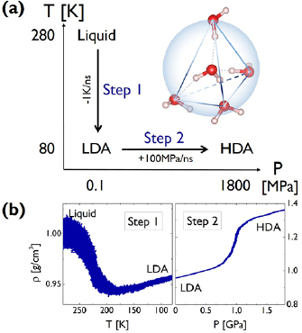
Figure 1. Amorphous ices generated by MD simulations. (a) Preparation routes for glassy water data on a T-P map. The inset figure depicts the local tetrahedral unit of water molecules based on H-bonds (gray dotted lines between O⋯H). (b) Change in density  along the transitions in the MD simulations, divided into two steps.
Download figure:
Standard image High-resolution imageAs such, most previous structural analyses of water have been limited to the short-range order (SRO) only. In amorphous water systems, SRO mostly refers to the size comparable to that of the local tetrahedral network frame, which is less than 3.0  while medium-range order (MRO) corresponds to the size range beyond that. In contrast to the SRO, our understanding of MRO in amorphous water systems still remains poor today. It has long been observed in x-ray or neutron diffraction experiments of water that the peak intensity in the structure factor increases as the temperature gets lowered, which directly implies an increase of MRO along the glass transition [14, 22]. In particular, for a glassy state of water below 120 K, the first sharp diffraction peak (FSDP) in the structure factor supports the existence of strong MRO features embedded in the amorphous system. To the best of our knowledge, however, the structural real space origin of those sharp peaks in the structure factor has not been clarified yet.
In this article, we combine two computational methods, molecular dynamics (MD) simulations and persistent homology (PH) in topological data analysis, to identify hidden MRO features in glassy water systems. The detected MRO structures are rings determined by the PH computing mechanism and are distinguished by their geometry, such as their size, shape and the number of components: MRO rings in LDA ice have larger size and flatter shapes, while involving less number of member atoms, than those in HDA ice. The ensemble of these MRO rings extracted from PH computations successfully reproduces the FSDP (both peak position and width) in the x-ray structure factor, demonstrating the ring structures as the real space origin of experimentally observed FSDPs. This result highlights that PH is a convincing tool to reveal a submerged order beyond the short local range in amorphous systems.
2. Methods
2.1. Molecular dynamics simulations
For MD simulations we used the TIP4P/2005 model [23] in the LAMMPS software [24]. We first prepared a liquid water structure as an isothermal-isobaric NPT ensemble of 2880 water molecules in a cubic box with periodic boundary conditions at  and
and  . The isobaric cooling cycle on the liquid water to obtain hyperquenched glassy water, i.e. LDA ice, ran for 200 ns at a cooling rate of
  ns−1. Then it is followed by the isothermal compression of LDA ice to get HDA ice at 1.3 GPa, running for 18 ns with a compression rate of 0.1 GPa ns−1. The time step for the integration algorithm was set to be 1 fs and the damping parameters for the thermostat and barostat are 0.5 and 5 ps, respectively. We cut off the Coulombic and Lennard-Jones interactions at distance 10
  and 10.3092
  , respectively [18].
2.2. Structure factor
The structure factor  measures the scattered intensity of an incident radiation for the scattering vector
  and is related to the radial distribution function (or pair correlation function) via the Fourier transform. For a perfect crystal, it exhibits infinitely many sharp peaks reflecting the periodicity of the system; for a liquid-like arrangement, a certain degree of fluctuations appears in the distribution function, yet the sharpness is weak. The numerical estimation of the structure factor of a multiatomic system of N atoms
  at positions
  is as follows [25]:
where  is the wave number for the wavelength
  of the plane wave and
is the (approximated) atomic form (or scattering) factor of each atom  with constants
  and cj reflecting the electron density of atom
  under the assumption that the electron density is spherically symmetric [26].
2.3. Topological analysis via persistent homology
For structural analysis, we used persistent homology (PH) computations from an emerging research field, topological data analysis [27, 28]. PH has been actively utilized in a wide range of domains, including materials science and neuroscience [29–34], as an effective detector of topological features, i.e. holes embedded in a system. For each dimension n, we define the nth persistent homology group PHn, which extracts qualitative features of n-dimensional holes, e.g. connected components for n = 0, rings for n = 1 and cavities for n = 2, that persist over multiple scales. Since we aim to detect MRO ring structures in water that are responsible for the FSDP in the structure factor, our focus is on the case n = 1.
As one of the most efficient representations of PH computations, a persistence diagram (PD) is used to visualize the distributions of size and shape of hole structures. PD can precisely reveal hierarchical structural units in various length scales from short- to long-range order in the system. In this sense, PD has great merit compared to other conventional methods for structural analyses, such as radial distribution functions (RDF), distributions of bond or dihedral angles and ring statistics [35]. The detailed PH computing mechanism for our study using HomCloud software [36, 37] follows in section 3.2 along with a schematic illustration.
3. Results
3.1. Data preparation and structure factor
We performed out-of-equilibrium MD simulations on the system of 2880 water molecules to obtain LDA and HDA ices, separated by two steps (figure 1(a)) as described in section 2.1. Figure 1(b) shows the change in density at each step, which is in good agreement with the experimental densities  0.95
0.95  and
and  1.31
1.31  at
at  and
and  GPa [5]. Note that we took LDA and HDA ice structures at P = 0.1 and
  , respectively, of which densities agree the best with the experimental results.
Next, the structure factor  of each glassy water system is computed and compared with experimental results [22] to confirm the reliability of our MD-generated amorphous ice systems. (See section 2.2 for the computational details.) For an amorphous configuration, the FSDP at small
  in
in  , if it exists, is closely related to MRO within the system [14, 38]. Figure 2 compares the experimental structure factor (top) with the computed
  (bottom) of our water structures generated by MD simulations. The FSDP position Q* in each case is well-matched to the experimental result at
  and
and  within the error bound of
 −1. Note that the position of the peak varies slightly from the experimental result due to the difference in external conditions of temperature and pressure in our simulation setup.

Figure 2. Structure factor. X-ray diffraction experiment results [22] (top) and computed  for the MD-generated data (bottom). The FSDPs of LDA and HDA ices are at
  and
and  , respectively.
Download figure:
Standard image High-resolution image3.2. Persistent homology computations
The PH computing mechanism is as follows. Suppose we have an atomic configuration of N atoms  centered at
  and a set
  of input radii. To compute PH1, we place a spherical ball of radius rj centered at
  , and enlarge the ball radius to
  with increasing
  , the scale parameter in the computation. When two balls meet, we add a line segment to connect the corresponding two atoms. As
  increases, more line segments appear and eventually create a ring by connecting multiple atoms end to end. When a ring
  is born,
  is recorded as the birth scale
  of the ring. In contrast, we define the death of ring
  when
when  is completely triangulated and every three balls has nonempty intersection. The
  at the death point is recorded as the death scale
  of the ring. The very last triangulated ring is called the death simplex, and its maximum side length represents the size of the ring. [31, 39]
Figure 3(a) shows a schematic illustration for the PH computing process with the resulting PD of a 2D version of a water configuration. In our study, we use the following input radii of atoms: taking the first peak positions 
 and
and 
 of the RDF of OH and HH pairs into consideration (figure S1 in supplementary data (stacks.iop.org/JPhysCM/31/455403/mmedia)), we solve the equations
  and
and  to take
 and
and 
 as the input radii of H and O atoms, respectively. As
  increases, growing balls intersect, thereby line segments connect atoms, so that multiple rings
  are created. Note that red triangles
  are small enough to disappear shortly after their birth, while the blue ring
  persists longest. In the PD, the longer a ring persists, the farther away it is placed from the diagonal. The largest ring
  has
has  for
for  as its subrings and the unfilled blue triangle at
  is the death simplex of
  .
.

Figure 3. Persistence diagrams PD1. (a) A schematic illustration of the construction of rings (left) over a 2D configuration with two different types of input radii and its resulting PD1 (right). (b) PD1 of LDA (left) and HDA (right). The colorbar represents the multiplicity of rings on a logarithmic scale. Both PDs have separated characteristic regions, denoted by Lj and Hj  .
.
Download figure:
Standard image High-resolution imageNext, the PD1 for our MD-generated amorphous ices are aligned in figure 3(b). Note that the birth–death pairs of rings in PDs are plotted in a squared scale of  2. PDs of both LDA and HDA ices show a division of points into distinct areas, characterized by lines or band-like regions, where a large number of points (each representing a ring) are concentrated. We denote the separated characteristic regions by Lj and
  for LDA and HDA, respectively, as depicted in the figure. Note that rings in vertical island regions L1 and H1 are composed of more than four member atoms (
 ) and their triangular or quadrilateral subrings are recorded in other regions close to the diagonal. Since rings in L4 and H4 are small triangles whose length scales contribute little to the FSDP in the structure factor, our focus is rather on rings in other characteristic regions (
 ) that would suitably correspond to the MRO in glassy water and are likely to be associated to the sharp peaks in
  in figure 2.
3.3. Characterizing MRO in LDA and HDA ices
The geometry of MRO ring structures of LDA and HDA ices substantially differs from each other in several aspects. First, stacked bar charts in figure 4(a) compare the distributions of the number of ring members ( ) in the vertical island regions L1 and H1 in PDs. We denote a ring with m members by m-ring. While L1 has a sharp distribution of the number of members, mostly concentrated on 7–10 members, H1 has a broader distribution, as many rings of H1 involve a larger number of atoms as their components. The median number of ring members is 9 and 12 in L1 and H1, respectively. As mentioned earlier, rings in other characteristic regions for
  (close to the diagonal) are simple triangles or 4-rings. We observe in figure 4(a) that HH atom pairs, as opposed to OH or OO (none) pairs, dominantly determine death scales of MRO rings both in LDA and HDA ices. The inset figures show six types of representative m-rings in L1 (
 –
– ) and in H1 (
 –
– ) extracted from the marked spots in the PDs in figure 3(b) with red lines connecting the atom pairs responsible for the death of each ring.
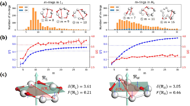
Figure 4. Ring analysis in L1 and H1. (a) Stacked bar charts show the distribution of the number of m-rings in L1 (left) and H1 (right) regions. The orange and blue bars count HH and OH atom pairs, respectively, that determine the death scale (hence the size) of rings. The inset figures are representative ring structures, corresponding to the blue spots  –
– in L1 and
  –
– in H1 in figure 3(b), with white H and red O atoms. (b) Red and blue line graphs display the change of the mean ring size
  and the mean degree of flatness
  , respectively, for L1 (left) and H1 (right). Error bar is defined as the standard error of the mean. Dotted lines represent the average values of
  and
and  of all rings. (c) Two 9-rings, each extracted from L1 (left) and H1 (right). The red triangle depicts the death simplex of each ring, and red dotted line connects the atom pair that terminates the triangulation of the ring.
Download figure:
Standard image High-resolution imageIn addition to the number of ring members, MRO rings in LDA and HDA ices are differentiated by their size and shape. For this purpose, we consider the following length of ring  :
:

which is the distance between the centers of atoms  and
and  , the pair of which determines the death scale
  of ring
  (i.e. depicted as red lines in figure 3(a)) [39]. Note that
  represents the size of
  , as
, as  is the maximum edge length within the triangulated ring, and is invariant under the choice of input radii, since it is determined by the given configuration itself. We plot red line graphs in figure 4(b) to show the mean value of
  of m-rings in L1 and H1 regions with respect to the number of ring members m, tending to increase as m becomes larger. The average sizes
  of the rings in L1 and H1 contributory to the FSDPs are estimated to be notably different as
 and
and 
 , respectively.
It might be counterintuitive that rings with more members in H1 are smaller than rings in L1 with fewer members. This is also confirmed in PDs where the death scale (i.e. the size of the ring) exhibits a range of smaller length scales in HDA than in LDA ice. However, as water molecules become closer to each other in HDA, mainly by the pressure effect, the movement naturally leads to smaller voids in twisted ring bodies with more members, which is consistent with higher density of HDA. We define the following formula to study the degree of flatness (or planarity) of a detected MRO ring  of m members:
where  is the position of atom
  and P is the best fit plane to the ring geometry that minimizes the sum of the distances of member atoms from the plane. Note that
  with F = 0 indicating that all the ring members are coplanar, hence a flat ring. MRO rings in L1 display flatter shapes with
 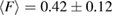 and
and  , while those in H1 have
 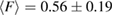 and
and  . The mean flatness
  of rings in L1 (left) and H1 (right) are shown with blue dotted lines in figure 4(b). Two 9-rings, each found in L1 and H1 regions, are shown in figure 4(c). This geometry is compatible to the picture where water molecules in the second coordination shell in the basic tetrahedral network penetrate into the first shell by the increased pressure, resulting in the deformed tetrahedral network in HDA ice.
3.4. Reproducing FSDPs by PD1 results
To reproduce the FSDP in  from PD1 results, we use the following equation [31]:
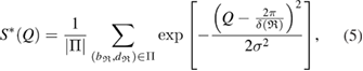
where  is a characteristic region Lj or
  on PDs with
  the number of rings in the region,
  is the birth–death pair of ring
  in a squared scale of
  2 and
2 and  applies a smoothing effect on the curve. Figure 5 shows the reproduced FSDPs of LDA (top) and HDA (bottom) by S*(Q). We first consider each individual characteristic region
  on PD to plot the corresponding S*(Q) and then their combination
  for each LDA and HDA ice. Note that rings in L1 and L2 regions contribute much to reproducing the peak at
  apart from the rings in L3 region, which are of smaller scale than those in other regions. This signifies that MRO rings in L1 and L2 are the main contributors to the FSDP in
  . Also in the case of HDA, the reproduced peak from the combined characteristic region
  matches fairly well with the designated spot.

Figure 5. Reproduced FSDP from PD1. Solid navy lines describe the reproduced peaks S*(Q) for the combined characteristic regions in the PD of LDA (top) and HDA (bottom). Dotted lines represent S*(Q) for the individual characteristic regions.
Download figure:
Standard image High-resolution image
In addition to the peak position, the width of the FSDP is also examined. We calculate the ratio 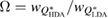 , where
  and
and  are the full widths at half maximum of the FSDPs of the amorphous ices. The ratio
  of the reproduced peaks is estimated to be 1.63, which excellently agrees with
  1.59 of the experimental data (top panel in figure 2) and
  1.60 of our MD-generated ice configurations (bottom panel in figure 2). All these values consistently reflect that the FSDP width of HDA ice is larger than that of LDA ice. Overall, PH-extracted MRO rings successfully reproduce the quantities associated with the FSDPs, including the peak positions and widths, in the structure factor, which convincingly supports that these rings construct the hidden MRO in glassy water, leading to the appearance of the sharp peaks.
In a multiatomic system as water, the larger the electron density of an atom has, the more effect it adds to the diffraction pattern. This fact has been one of the reasons for higher attention to the oxygen arrangement only in the previous studies of water structures [17, 40]. As a comparison, we further carried out the FSDP reconstruction process based on the oxygen arrangement only (O-system hereafter) and compared the results to the case of the entire H2O system (figure S2 in supplementary data). While the trend of the FSDP of HDA appearing at larger Q than that of LDA is preserved, O-system does not accurately reproduce the quantities associated with the FSDP (e.g. peak position and width). For the O-systems in the bottom panel in figure S2, the peak positions deviate by approximately 0.4–0.6  −1, and also the notably larger peak width of HDA than that of LDA is not reproduced. Thus, it is critical to keep both oxygen and hydrogen atoms into consideration for an accurate PH analysis of water in ensemble. This is a hitherto unknown result, which would have been difficult to obtain in earlier approaches, as previously known structural information was mostly based on oxygen atoms in water, overlooking hydrogen atoms as a mere decoration.
4. Conclusion
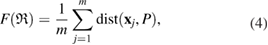
In conclusion, our combined approach using MD and PH has successfully embodied the real space origin of the FSDP in the structure factor of both types of amorphous ices by detecting MRO ring structures in each. We identified the MRO structures via separated regions in PDs and compared those in each type of the amorphous ice systems in terms of their shape and size as well as the number of ring constituents. The average ring size  and the average degree of flatness
  of the rings can be summarized as
  and
and  . The PH-extracted MRO rings well explain the quantitative features (peak position and width) of the FSDPs in the structure factor, hence suitably serve as a hidden order in real space. Further applications of PH will shed light on our fundamental understanding of various types of amorphous systems with interesting MRO features that are yet hidden in a complicated geometry.
Acknowledgments
This work was supported by KIST institutional grant (2E29280) and Creative Materials Discovery Program (NRF-2016M3D1A1021140) and Nano Material Technology Development Program (NRF-2016M3A7B4024131) through the National Research Foundation of Korea. SH is grateful to Yasuaki Hiraoka at Kyoto University and to Tomohide Wada at Tohoku University for their instruction on TDA applications in materials science.
Author contributions
S H and D K designed research and wrote the paper; S H performed M D simulations and obtained computational results.