

Abstract
Many-body perturbation theory is often formulated in terms of an expansion in the dressed instead of the bare Green's function, and in the screened instead of the bare Coulomb interaction. However, screening can be calculated on different levels of approximation, and it is important to define what is the most appropriate choice. We explore this question by studying a zero-dimensional model (so called 'one-point model') that retains the structure of the full equations. We study both linear and non-linear response approximations to the screening. We find that an expansion in terms of the screening in the random phase approximation is the most promising way for an application in real systems. Moreover, by making use of the nonperturbative features of the Kadanoff–Baym equation for the one-body Green's function, we obtain an approximate solution in our model that is very promising, although its applicability to real systems has still to be explored.
Export citation and abstract BibTeX RIS
1. Introduction
In an interacting electron system, complete knowledge of the many-body wavefunction allows one to calculate all expectation values and therefore to determine all observables. However, in most cases it is neither possible nor desirable to calculate the full wavefunction, as in the calculation of the observables much details of the wavefunction are integrated out. In particular, expectation values of one-body operators and the total energy can be obtained in a straightforward way from the one-body Green's function  , which is itself an expectation value of an electron creation and an annihilation field operator. This Green's function can be expressed as a series whose terms only include its non-interacting counterpart
  and the Coulomb potential
  .
.
Such a series, however, can be badly behaved, as, for instance, in the case of extended systems in the thermodynamic limit. In these situations, one can still extract sensible estimates of the Green's function by summing up an infinite subset of terms of the series. The cornerstone of this approach is the Dyson equation, which in a simplified notation reads  ; here the focus is shifted on the self-energy Σ, whose perturbative expansion is still expressed in terms of G0 and vc only. Any finite truncation of the series for Σ leads to a resummation of an infinite number of terms in the series of G, and only a few terms of the series of Σ are usually sufficient to greatly improve on truncations of the series of G itself. Still, in order to obtain satisfactory spectra, at least in an extended system it is not sufficient to keep for the self-energy only some diagrams of low order in G0 and vc. In particular, it has rapidly been realized that one should resum diagrams that dress the bare Coulomb interaction, since the effective interaction between charges is usually strongly screened.
In extended systems at zero temperature, the state of the art approach for the calculation of G, and hence of electron addition and removal spectra, is the so-called GW approximation (GWA). In a seminal paper, Hedin formalized this idea by introducing an appropriate screened interaction W and expressing the exchange-correlation contribution  to the self-energy as a functional of G and W, rather than G0 and vc. He derived the expression using Schwinger's functional derivative idea, where all the information about exchange and correlation effects on the one-body and higher order Green's functions are contained in a functional differential equation that involves the response of the system to a fictitious external potential [1, 2]. From the differential equation, a set of five equations are derived that are known as 'Hedin's equations' [3]. They contain the one-body Green's function G, the self-energy Σ, the irreducible polarizability P which gives rise to the screened Coulomb interaction W, and a vertex function Γ which stems from variations of the self-energy. The GWA arises as the first step of an iterative procedure that formally solves Hedin's equations. This first approximation corresponds to setting the vertex
  . The GWA has encountered large success, in particular concerning the calculation of band gaps. However, in cases of failure, such as the description of Mott insulators which come out metallic in GW [4], or the absence of satellites related to excitations that are not due to the formation of electron-hole pairs [5], a straightforward further iteration of Hedin's equations has not yet proved to be successful, and, for many applications, it is not even feasible.
The power of the GWA is generally attributed to the belief that the screened Coulomb interaction W is weaker than the bare vc, and that therefore a perturbation expansion in W should be more powerful than an expansion in vc. This, however, is not necessarily true. To see the point, it is sufficient to consider the screening due to a single electron in some potential. In this case the density–density response function χ is simply the non-interacting response function  . The inverse dielectric function
  , which screens the Coulomb interaction via the relation
  , becomes
  . Since
  is negative, W is indeed often smaller than vc. However, for large enough (negative)
  compared to
  the inverse dielectric function and W become negative, and their absolute value can be arbitrarily large. In this case the argument in favor of a perturbation expansion in terms of W breaks down. Instead, this scenario never happens when W is calculated in the random phase approximation (RPA), where only variations of the Hartree potential screen the interaction. In the RPA the dielectric function is
  , which is always positive and larger than 1, such that the resulting screened interaction
  . This suggests that an expansion in terms of the RPA W0 might be more powerful than an expansion in W. This indicates a first route to obtain improved expressions, which we follow in the present work.
Instead of searching for a perturbation expansion for the self-energy, one may also go back to the starting point, a functional differential equation. Here we use the Kadanoff–Baym equation (KBE) [6], which can be reformulated such that screening appears explicitly. The GWA is obtained from this equation as a linear-response approximation in conjunction with an approximation on variations of the Green's function with respect to the total classical potential. Also the widely used second-order cumulant approximation can be derived from this equation, again using the linear response approximation, but introducing a decoupling approximation between different states instead of the approximation on the variations of G. In order to go beyond both approximations, it is therefore in particular interesting to investigate contributions beyond linear response.
In the present work, both ideas are explored using a simple model, the 'One-Point model' (OPM). Such a mathematical toy model, which has already been used in a similar context [7–9], represents the zero-dimensional version of a generalized Kadanoff–Baym equation. The model captures many features of the original, multi-dimensional case; it incorporates, for instance, the failure of the skeleton series that was only recently found for some multi-dimensional cases [10–12]. The model is exactly solvable, and it reflects many features of findings for real systems, such as the quality of various approximations [13]. Therefore, it constitutes an established first step to test new approximations.
The paper is organized as follows. Section 2 will be devoted to recall the reader the theoretical framework; our two approaches will be motivated and presented in sections 3 and 4, respectively; results of tests on the OPM are presented in section 5; feasibility and computational cost of the approaches for real systems will be discussed in section 6 where conclusions will also be drawn.
2. The equation of motion and the functional approach
In a non-interacting system, one can determine the one-body Green's function G0 from its equation of motion (EOM), which is a differential equation containing the first-order time derivative of the Green's function and the single-particle Hamiltonian. Together with a boundary condition in time, this fully determines G0. In an interacting system, the EOM for the one-body Green's function G contains additional contributions due to the interaction: besides the Hartree potential, a two-body Green's function appears, which contains the information about exchange and correlation between the interacting particles. In turn, the EOM of the two-body Green's function contains the three-body Green's function, and one finds an infinite chain of equations [4].
The equations can be cast into a more compact form by using the fact that higher-order Green's function s can be expressed as variations of the one-body G with respect to an external potential φ. This allows one to write the EOM for the one-body Green's function G as
where vc is the Coulomb potential, 
 is the Green's function of the noninteracting system, and the Hartree potential
 ![$ V_{{\rm H}}(1;[\varphi])$](https://content.cld.iop.org/journals/0953-8984/30/13/135602/revision2/cmaaaeabieqn018.gif) is
is
Here, we use  as a short-hand notation to combine the space, spin, and time variables. Moreover,
  , where
  with
with  .
.
In equation (1) the generalized one-body Green's function ![$G(1, 2; [\varphi])$](https://content.cld.iop.org/journals/0953-8984/30/13/135602/revision2/cmaaaeabieqn023.gif) is a functional of a time-dependent external potential
is a functional of a time-dependent external potential  . The equilibrium one-body Green's function of interest is retrieved in the limit of vanishing
  . Without the last term on the right-hand side of equation (1), this equation would be the Dyson equation in the Hartree approximation. All the many-body effects (exchange and correlation (xc)) beyond the Hartree potential are contained in the derivative term.
As pointed out by Baym and Kadanoff in [6], there is no known way to solve this equation. In particular, such a non-linear multi-dimensional functional integro-differential equation can have many solutions, and it may be difficult to chose which one is physical. Usually, the problem is circumvented by using some kind of iterative approach, starting from the non-interacting or the Hartree solution. A straightforward iteration of equation (1) leads to series of terms of increasing order in the interaction and corresponds to a perturbation expansion of G. However, such a series has often bad convergence properties (see also section 5 for an illustration). Therefore a common way to go is to transform equation (1) into a Dyson equation:
with the exchange-correlation self-energy
Here and in the following, we denote integrals by  .
.
Once the expression for the self-energy is established, it is enough to solve equation (3) for  in order to obtain the equilibrium Green's function. Of course, since G is unknown so is
  : with the transformation of the EOM into a Dyson equation, the goal becomes to find accurate approximations to the self-energy. The advantage of the Dyson equation is the fact that even a low-order approximation to the self-energy creates in the Green's function terms to infinite order in the interaction, so one may hope that approximating
  is easier than approximating G itself.
One strategy to find approximations for  has been formalized by Hedin [3], based on the insight that, at least for extended systems, screening of the interaction plays a key role. The screening is due to the self-consistent reaction of the electron system to the variation of the external potential. This self-consistency is automatically taken into account when the variation of the total, i.e. external plus system-internal, potential is considered. Hedin's formulation uses the classical part of the total potential,
  , to express the exact exchange-correlation self-energy (4) as
with

and the irreducible polarizability

From the Dyson equation (3), the fifth equation in Hedin's set is derived for the irreducible vertex function  as
as
The screened Coulomb interaction W is linked to the density–density response function
via  , and it can also be expressed in terms of the inverse dielectric function
  as
as

By setting  , the equations reduce to a closed set of algebraic equations for G, Σ, W and P, leading to the so called GWA for the self-energy and the RPA for P. The equations can now be solved self-consistently. Often, however, some mean-field Green's function is used instead of the self-consistent G to build the self-energy. The mean-field Green's function is usually referred to as G0, although it contains some interaction through, e.g. the KS potential or the Fock exchange. This approach is usually called
  . For later reference we highlight the fact that W is calculated in the RPA by using the notation

where the RPA functional is ![$ \newcommand{\Wrpa}[1]{\mathcal{W}_{\rm RPA}[#1]} \newcommand{\e}{{\rm e}} \Wrpa{F}\equiv (1+{\rm i}FFv_{\rm c}){\hspace{0pt}}^{-1}v_{\rm c}$](https://content.cld.iop.org/journals/0953-8984/30/13/135602/revision2/cmaaaeabieqn037.gif) . Such a functional generalizes the functional form of W obtained from the RPA for P, where
. Such a functional generalizes the functional form of W obtained from the RPA for P, where  implies
  and hence
  .
.
The  scheme has led to good results in many cases, but it suffers from the fact that these results strongly depend on the choice of the mean field in G0. For this reason, partially self-consistent schemes have been developed and led to important progress. Technically, even fully self-consistent GW calculations are nowadays feasible [14]. However, it is not clear whether full self-consistency on the GW level is desirable; in particular, it has been pointed out that the resulting χ does not fulfil the f-sum rule [15]. Clearly, vertex corrections, i.e. corrections to the self-energy of higher order in W, are needed to improve this situation.
3. Perturbation theory in W0
The success of the GWA may be explained by the intuitive picture according to which the screened potential W represents a better parameter than the bare Coulomb interaction vc for a perturbative expansion of  . This presumes that
  . Although often true, this is simplistic, and as explained in the introduction
  can in principle become arbitrarily large. On the other hand,
 ![$P^{\rm RPA}(\omega=0;[G_0])$](https://content.cld.iop.org/journals/0953-8984/30/13/135602/revision2/cmaaaeabieqn045.gif) built with any mean-field G0 is always negative, which means that
built with any mean-field G0 is always negative, which means that ![$ \newcommand{\Wrpa}[1]{\mathcal{W}_{\rm RPA}[#1]} \Wrpa{G_0}$](https://content.cld.iop.org/journals/0953-8984/30/13/135602/revision2/cmaaaeabieqn046.gif) is always positive and smaller than vc. Moreover, the corresponding density-density response function
is always positive and smaller than vc. Moreover, the corresponding density-density response function ![$\chi^{\rm RPA}[G_0]$](https://content.cld.iop.org/journals/0953-8984/30/13/135602/revision2/cmaaaeabieqn047.gif) is well behaved; in particular, it fulfils the f-sum rule.
is well behaved; in particular, it fulfils the f-sum rule.
Based on these considerations, we propose to consider the perturbative expansion of  in G0 and
 ![$ \newcommand{\Wrpa}[1]{\mathcal{W}_{\rm RPA}[#1]} \Wrpa{G_0}$](https://content.cld.iop.org/journals/0953-8984/30/13/135602/revision2/cmaaaeabieqn049.gif) . This is formally constructed in the following way. First, we use the definition of
. This is formally constructed in the following way. First, we use the definition of ![$ \newcommand{\Wrpa}[1]{\mathcal{W}_{\rm RPA}[#1]} \Wrpa{G_0}$](https://content.cld.iop.org/journals/0953-8984/30/13/135602/revision2/cmaaaeabieqn050.gif) to invert the map
to invert the map ![$ \newcommand{\Wrpa}[1]{\mathcal{W}_{\rm RPA}[#1]} v_{\rm c} \to \Wrpa{G_0}$](https://content.cld.iop.org/journals/0953-8984/30/13/135602/revision2/cmaaaeabieqn051.gif) , which leads to
, which leads to ![$ \newcommand{\Wrpa}[1]{\mathcal{W}_{\rm RPA}[#1]} v_{\rm c}=(\Wrpa{G_0}^{-1} + P_0){\hspace{0pt}}^{-1}= $](https://content.cld.iop.org/journals/0953-8984/30/13/135602/revision2/cmaaaeabieqn052.gif)
![$ \newcommand{\Wrpa}[1]{\mathcal{W}_{\rm RPA}[#1]} \Wrpa{G_0}(1-{\rm i}\Wrpa{G_0}G_0G_0){\hspace{0pt}}^{-1}$](https://content.cld.iop.org/journals/0953-8984/30/13/135602/revision2/cmaaaeabieqn053.gif) with
with  . We then use the well established perturbation expansion of
  in terms of vc and insert the above expression for vc to rewrite the series in terms of
 ![$ \newcommand{\Wrpa}[1]{\mathcal{W}_{\rm RPA}[#1]} \Wrpa{G_0}$](https://content.cld.iop.org/journals/0953-8984/30/13/135602/revision2/cmaaaeabieqn056.gif) and, finally, we group terms of the same order in
and, finally, we group terms of the same order in ![$ \newcommand{\Wrpa}[1]{\mathcal{W}_{\rm RPA}[#1]} \Wrpa{G_0}$](https://content.cld.iop.org/journals/0953-8984/30/13/135602/revision2/cmaaaeabieqn057.gif) . By defining
. By defining ![$ \newcommand{\Wrpa}[1]{\mathcal{W}_{\rm RPA}[#1]} \newcommand{\e}{{\rm e}} W_0\equiv \Wrpa{G_0}$](https://content.cld.iop.org/journals/0953-8984/30/13/135602/revision2/cmaaaeabieqn058.gif) we can schematically represent the procedure as
we can schematically represent the procedure as
Being more specific, if the starting G0 is, for instance, the Hartree Green's function GH we have that
where ![$ \newcommand{\Wrpa}[1]{\mathcal{W}_{\rm RPA}[#1]} \newcommand{\e}{{\rm e}} W_{\rm H}\equiv \Wrpa{G_{\rm H}}$](https://content.cld.iop.org/journals/0953-8984/30/13/135602/revision2/cmaaaeabieqn059.gif) . The first term represent the GWA, while the others, between brackets, the second order contribution in WH. Diagrammatically, this is represented by
. The first term represent the GWA, while the others, between brackets, the second order contribution in WH. Diagrammatically, this is represented by
4. Nonperturbative linear response
The previous section designs a way to use a linear response ingredient, namely W0, in order to build more powerful perturbation series. In the present section we will discuss a way to make non-linear response appear. Since the expressions become quickly very clumsy, we suppress in the presentation all arguments except for the functional dependence on the fictitious external potential, which is crucial for the derivations.
Starting from (1), we focus on the self-energy
We assume that ![$V_{\rm H}[\varphi]$](https://content.cld.iop.org/journals/0953-8984/30/13/135602/revision2/cmaaaeabieqn060.gif) (defined in (2)) is Taylor expandable:
(defined in (2)) is Taylor expandable:
where ![$ \newcommand{\e}{{\rm e}} n(1)\equiv G(1, 1^+;[0])$](https://content.cld.iop.org/journals/0953-8984/30/13/135602/revision2/cmaaaeabieqn061.gif) is the charge density. As first approximation, we truncate the above series to first order
is the charge density. As first approximation, we truncate the above series to first order
which leads to
This rewriting suggests to renormalize (or screen) the external potential as
Since (18) implies
with ![$ \newcommand{\e}{{\rm e}} \bar{G}[\bar{\varphi}]\equiv G[\varphi[\bar{\varphi}]]$](https://content.cld.iop.org/journals/0953-8984/30/13/135602/revision2/cmaaaeabieqn062.gif) , we can write (17) as
, we can write (17) as
The functional derivative can be approximated with the leading order of its perturbative expansion in ![$\bar{G}[\bar{\varphi}]$](https://content.cld.iop.org/journals/0953-8984/30/13/135602/revision2/cmaaaeabieqn063.gif) , as5
, as5
Combining (23) and (24) one finds
Since the derivative part has been approximated, this equation is no longer a functional–differential equation but a Dyson equation, which can be solved directly at  . The equilibrium self-energy is then obtained as
since ![$\bar{G}[0]=G[0]$](https://content.cld.iop.org/journals/0953-8984/30/13/135602/revision2/cmaaaeabieqn070.gif) . Here the RPA screened interaction appears, since
. Here the RPA screened interaction appears, since
where f denotes a generic function on which the operator  acts. Since
 ![$\bar{G}[0]=G[0]$](https://content.cld.iop.org/journals/0953-8984/30/13/135602/revision2/cmaaaeabieqn072.gif) the self-energy (26) becomes
the self-energy (26) becomes

These are, respectively, the self-consistent GWA with ![$ \newcommand{\Wrpa}[1]{\mathcal{W}_{\rm RPA}[#1]} W\approx\Wrpa{G}$](https://content.cld.iop.org/journals/0953-8984/30/13/135602/revision2/cmaaaeabieqn073.gif) , and the so-called
, and the so-called  approximation, where the expressions are evaluated with non-interacting Green's functions; in practice, most often some mean-field solution such as a Kohn–Sham Green's function is used for G0.
The above derivation of the  approximation relies on two ordered approximations: (16) and (24), that are tied to each other via the definition of the screened perturbing potential
  . The first one makes the problem linear, while the second one removes the differential character and leads to an algebraic equation. If one would apply (24) directly on (14), without going through (16) and the definition of
  , one would get to

which is simply the Hartree–Fock approximation.
The derivation seems to suggest that a better approximation may come from improving on (16), namely taking more orders of the Taylor expansion of ![$V_{\rm H}[\varphi]$](https://content.cld.iop.org/journals/0953-8984/30/13/135602/revision2/cmaaaeabieqn078.gif) . However, solving the Dyson equation at equilibrium kills all possible improvements. Such a mechanism is clear already when keeping the second order in (15). Let us first write
. However, solving the Dyson equation at equilibrium kills all possible improvements. Such a mechanism is clear already when keeping the second order in (15). Let us first write
Now we introduce the screened perturbing potential (in the even shorter notation for which functional derivatives ![$\delta F[\varphi]/\delta \varphi$](https://content.cld.iop.org/journals/0953-8984/30/13/135602/revision2/cmaaaeabieqn079.gif) are denoted by
are denoted by ![$F'[\varphi]$](https://content.cld.iop.org/journals/0953-8984/30/13/135602/revision2/cmaaaeabieqn080.gif) )
)
for which
where ![$ \newcommand{\e}{{\rm e}} \tilde{G}[\tilde{\varphi}]\equiv G[\varphi[\tilde{\varphi}]]$](https://content.cld.iop.org/journals/0953-8984/30/13/135602/revision2/cmaaaeabieqn081.gif) . This implies that
. This implies that

which, in combination with
gives
which at equilibrium is just

It follows that the only way to include non-linear screening effects is to go beyond the second approximation (24) and (34). This suggests that in order to go beyond the GWA one should keep the functional derivative, and attempt to solve the linearized functional–differential equation itself, as it has been suggested in [9] and pursued in [16, 17] in the context of cumulant approximations.
According to the order of the truncation of (15), we get different approximate KBEs, which we shall collectively refer to as 'hierarchy of linearized KBEs', since these differential equations are linear in the variable ![$G[\varphi]$](https://content.cld.iop.org/journals/0953-8984/30/13/135602/revision2/cmaaaeabieqn082.gif) . The coefficients of the Taylor expansion can in principle be estimated within time-dependent density functional theory (TDDFT), or evaluated self-consistently once the differential equation is solved6. The hope is that one recovers the original KBE by climbing the hierarchy of linearized KBEs, namely by considering more and more terms of (15), and that the resulting hierarchy of physical solutions to these equations smoothly converges to the exact Green's function.
. The coefficients of the Taylor expansion can in principle be estimated within time-dependent density functional theory (TDDFT), or evaluated self-consistently once the differential equation is solved6. The hope is that one recovers the original KBE by climbing the hierarchy of linearized KBEs, namely by considering more and more terms of (15), and that the resulting hierarchy of physical solutions to these equations smoothly converges to the exact Green's function.
5. Tests on the OPM
Iterating the KBE (1) starting from the (solvable) case  gives rise to the perturbative expansion of the Green's function. Apart from that, there are no standard techniques to solve the equation, preventing us to extract information on the Green's function in its nonperturbative regime. Even worse, the equation admits an infinity of solutions and it is unclear what sort of condition should be added to identify the desired one. In recent years, it has been suggested to reduce the complexity of the problem by looking at the zero-dimensional version of the equation [9]. The equation would retain its differential character, but rather than functionals one would have to deal with simple functions of one variable. In particular, with the substitution
 ![$G(1, 2;[\varphi])\to {\rm i}y(x)$](https://content.cld.iop.org/journals/0953-8984/30/13/135602/revision2/cmaaaeabieqn084.gif) ,
, ![$G_0(1, 2[\varphi])\to y_0(x)$](https://content.cld.iop.org/journals/0953-8984/30/13/135602/revision2/cmaaaeabieqn085.gif) ,
,  ,
,  the equation reads
  . The interacting zero-temperature equilibrium Green's function would then be represented by the value of the function(al) y at vanishing external field x, namely
  . Such an equation is, however, too simple: its iteration leads to the solution y(0) = y0(0), i.e. the interacting Green's function equals the noninteracting one. A way to add some complexity of the original multidimensional problem is to avoid the perfect cancellation occurring between the Hartree and the exchange-correlation self-energy in zero dimensions. This is achieved by introducing a parameter λ:
  . We refer to the resulting equation as the one-point model (OPM). Inspired by Hartree–Fock, in which only like spins are affected by exchange interaction, the specific value
  was considered [13]. With such a choice the model can be solved explicitly: Iteration of the equation with
  leads to a perturbative expansion that is non-trivial but still simple enough to be summed up in a closed form, as we shall later see. The resulting function
  , which represents the OPM version of
 ![$G(1, 2;[\varphi])$](https://content.cld.iop.org/journals/0953-8984/30/13/135602/revision2/cmaaaeabieqn094.gif) , is now complex enough to discuss several aspects of the original multidimensional problem. In fact, despite its simplicity, the OPM with
, is now complex enough to discuss several aspects of the original multidimensional problem. In fact, despite its simplicity, the OPM with  has proved to be a surprisingly reliable benchmark for qualitative analysis of approximation schemes, as proved by the analyses performed by Berger et al [13] and, later, Stan et al [12], who also showed that the model can be used to study pathologies of perturbation theory such as the misconvergence of the skeleton series [10]. This makes the model particularly appropriate for the study of the nonperturbative features of the equation of motion and its approximations, discussed in the previous section. Moreover, one can also use it to test perturbative schemes like the one based on an expansion in the RPA screened interaction, with the possibility of exploring at glance a large number of terms of a series and getting qualitative insights concerning its convergence.
In the next subsections, we shall recall the relevant ingredients of the OPM (section 5.1); show the performance of the OPM equivalent of GWA (section 5.2), which will serve as benchmark for our suggested approximations; derive and study the series in the equivalent of ![$ \newcommand{\Wrpa}[1]{\mathcal{W}_{\rm RPA}[#1]} \Wrpa{G_0}$](https://content.cld.iop.org/journals/0953-8984/30/13/135602/revision2/cmaaaeabieqn096.gif) and compare it with the series in the exact W (section 5.3); solve the hierarchy of the OPM equivalent of the linearized KBE (section 5.4); and, finally, compare all approaches (section 5.5).
and compare it with the series in the exact W (section 5.3); solve the hierarchy of the OPM equivalent of the linearized KBE (section 5.4); and, finally, compare all approaches (section 5.5).
5.1. The one-point model
We here summarize the relevant features of the OPM. The reader interested to more details is referred to the work of Berger [13]. At the basis of the model we find the differential equation:

with  ,
,  ,
,  ,
,  ,
,  . For
. For  , the above equation corresponds to the zero-dimensional version of the equation of motion (1), provided that


For this specific value of λ, the exact problem is characterized by the trivial physical solution y(x) = y0(x). A much richer result is obtained by considering  . Here we take
  , namely

The choice  reflects the fact that in the real system Hartee and exchange contributions do not cancel perfectly, whereas this would be the case in the model for
  . In this sense,
  is linked to the prefactor 1/2 that is often used in real systems for exchange terms when spin is not explicitly considered.
In analogy with the original problem, one can use the equation to get the perturbative expansion of  in v without actually solving the differential problem. In fact, the resulting series:
can be summed up to the function
which is the analytic continuation of the series (40). Since (41) is also solution to (39), we identify this as the physical solution of the problem, all other solutions to (39) being labeled as unphysical ones. Such a function is a model of the functional that in the standard many-body problem realizes the map  by analytic continuation of the series produced by perturbation theory. The Green's function at equilibrium, namely
 ![$G[\varphi = 0]$](https://content.cld.iop.org/journals/0953-8984/30/13/135602/revision2/cmaaaeabieqn110.gif) , is then represented by
, is then represented by
which is plotted in figure 1. The function y0(x), to which yp(x) reduces for  , is then identified as the out-of-equilibrium non-interacting Green's function, the corresponding version at equilibrium being simply
  . Provided with these functions, we can define the physical self-energy Σ, the Hartree self-energy
  , the exchange-correlation self-energy
  , the screened potential w and the RPA function(al)
  as
as


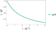
Figure 1. The function yp(x) represents the functional ![$G[\varphi]$](https://content.cld.iop.org/journals/0953-8984/30/13/135602/revision2/cmaaaeabieqn116.gif) , therefore the equilibrium Green's function, which is the values of the functional at
, therefore the equilibrium Green's function, which is the values of the functional at  , is represented by yp(0). A specific value of yp(0) is determined by v, which represents the coupling between the electrons, and
  , which represents the non-interacting Green's function and encodes all information of the non-interacting system. In analogy with the study of the Hubbard model, we can consider fixed (say
  ) and let v > 0. While varying, v spans a 'weakly coupled regime'
  , a 'strongly coupled regime'
  , and an intermediate region. The notation '
![$y\;[y_0^0]$](https://content.cld.iop.org/journals/0953-8984/30/13/135602/revision2/cmaaaeabieqn122.gif) ' and '
' and '![$v\;[y_0^0{\hspace{0pt}}^{-2}]$](https://content.cld.iop.org/journals/0953-8984/30/13/135602/revision2/cmaaaeabieqn123.gif) ', here and in all following plots, is a reminder that the problem can be entirely rewritten in terms of the adimensional quantities
', here and in all following plots, is a reminder that the problem can be entirely rewritten in terms of the adimensional quantities  and
and  and therefore y can be expressed in units of
  and v in units of
  .
.
Download figure:
Standard image High-resolution imageIn the rest of the section we shall consider  as given once for all. This is different from the work of Berger where
  was calculated self-consistently. We make this choice since it will allow us to better represent standard many-body techniques, and
  in particular, in which
  is usually a given input coming from a DFT calculation. Moreover it allows us to discuss the two proposed schemes in a consistent way.
5.2. The GW approximation (GWA)
To assess the quality of the proposed approximations, we shall compare them with the OPM equivalent of the GWA. A thorough analysis of such an approximation was worked out by Berger [13], who considered a self-consistently calculated  . As pointed out above, here we make an analogous analysis, but with a
  which is supposed to be given. The self-consistent GWA corresponds to solving the set of equations


This set of equations admits three solutions, of which only the following reduces to  in the noninteracting limit:
with

For real systems a direct solution of the GW equations is, in general, not feasible. Therefore, in practice, they are usually solved iteratively. Since the GW equations can be rewritten in several ways, various iterative schemes are possible [13]. Interestingly, the above solution can be obtained by the following iterative procedure:


starting from  , which is the standard iterative scheme used in GW calculations for real systems. We note that the above iterative scheme converges to the physical solution for all v thanks to the fact that we consider
  fixed. Otherwise the above iterative scheme does not converge for large v [13].
Since we can also calculate the exact screened potential W, it is worthwhile to explore also a GW self-energy built with the exact W, which could in principle be obtained from TDDFT. In this case, we solve the Dyson equation (44c) with the exact screened potential W = w of (43f). Of the two solutions, the only one that goes to zero in the limit  is
is
In figure 2, the OPM equivalent of the self-consistent GWA and self-consistent GW with W exact are shown in comparison with the equivalent of  . We include the case derived here, where the self-consistency is performed keeping vH fixed where vH is calculated self-consistently. We notice that this latter, which obeys to
and was studied in [13], leads to the best of all GW-like approximations.
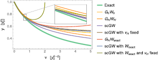
Figure 2. Comparison of the Green's function calculated using various flavours of the GWA with the exact solution, as a function of the interaction:  ,
,  starting from Hartree Green's function, self-consistent GW (where vH is calculated self-consistently, as in [13], self-consistent GW with vH fixed to its exact value, GW with Hartree G and W fixed to its exact value, GW with self-consistent G and W fixed to its exact value, GW with self-consistent G and W and vH fixed to their exact values.
Download figure:
Standard image High-resolution image5.3. Perturbation theory in W0 and W
The function yp(0), which represent the equilibrium interacting Green's function, is written in terms of two parameters:  , which represents the equilibrium non-interacting Green's function, and v, which parametrizes the interaction. Following section 3, we can rewrite it in terms of
  and
and  by simply using the definition of wrpa to express v, which leads to

Similarly, we can express Σ and  as
as
In figure 3, we compare approximations to yp(0) resulting from the straight perturbative expansion (51) and from the solution to the Dyson equation with self-energy approximated by the expansion in (52). All hierarchies of approximations smoothly converge to the correct result. It is worth noticing that, even though the leading order expansion of  gives a better approximation for large values of v compared with the other leading orders, the straight expansion of yp(0) converges much faster than the others.
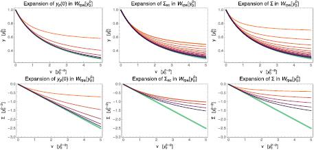
Figure 3. Top panels: the exact yp(0), in green, and the hierarchy of approximations obtained by using truncations of the series in wrpa, given by equations (45)–(47), respectively, in shades of orange (the darker the shade the higher the order of the truncation). Bottom panels: the exact self-energy Σ, in green, and the self-energies corresponding to the above approximations, in the same shades of orange.
Download figure:
Standard image High-resolution imageIf the starting point of the GWA is not the completely noninteracting Green's function, but rather the Hartree one, here defined by  , then the expansion is performed in
 ![$ \newcommand{\Wrpa}[1]{\mathcal{W}_{\rm RPA}[#1]} \newcommand{\e}{{\rm e}} w_{\rm H}\equiv \Wrpa{y_{\rm H}}$](https://content.cld.iop.org/journals/0953-8984/30/13/135602/revision2/cmaaaeabieqn147.gif) :
:

which also shows a good convergence, as reported in figure 4.

Figure 4. The exact yp(0), in green, and the hierarchy of approximations obtained by using trunctions of the series in the exact screening W, given by equations (49)–(51), respectively, in shades of blue (the darker the shade the higher the order of the truncation).
Download figure:
Standard image High-resolution imageFinally, we would like to reply to the question: is the exact W a better parameter than wrpa? Even though for real systems the exact W is not accessible, an affirmative reply to this question would justify the search for better approximations by incorporating vertex corrections into W. To find an answer within our model, we have to invert the expression (43f) to get the function corresponding to the map w, the exact screening of the OPM, to v. There are three solutions to the equation for v, of which only one goes to 0 when W goes to 0, namely
with  and
and  . Provided with such a map, we can calculate again the expansion of yp(0),
  and Σ to be
Truncations of the above series are plotted in figure 6. Few orders of the series are representative of the overall bad behaviour of the series. This suggests that the exact W does not represent a good parameter for a perturbation expansion. Indeed, a glance at the comparison of the RPA and the exact inverse dielectric function in figure 5 shows that while the RPA value is steadily decreasing with increasing interaction, the tendency is inverted starting from a critical value of the interaction in the exact case, making the screened interaction too large to be a useful parameter for perturbation theory.

Figure 5. The exact inverse of the dielectric function, defined as  , compared to its RPA equivalent
  .
.
Download figure:
Standard image High-resolution image
Figure 6. The exact yp(0), in green, and the hierarchy of approximations obtained by using trunctions of the series in the exact screening W, given by equations (49)–(51), respectively, in shades of blue (the darker the shade the higher the order of the truncation).
Download figure:
Standard image High-resolution image5.4. Solutions to the hierarchy of linearized KBE
We will now move on to the second route beyond the standard approximations, namely the expansion of the Hartree potential introduced in section 4. To this end, we define the the 'perturbed' Hartree potential as  , which leads to rewrite (39) as

and consider the hierarchy of approximations generated by truncating its Taylor expansion in the perturbing potential

The leading term V0 simply corresponds to the  previously defined and assumed to be known, while the other terms involve derivatives of
  evaluated at zero: V1 = −vy'(0), V2 = −vy"(0)/2, etc which are not known a priori. Just like for V0, we could consider them as given inputs, since for real systems they can in principle be obtained within the framework of TDDFT. In practice, however, we can only get approximations to their value, on which we have no control. We therefore prefer to calculate them self-consistently within our scheme. To simplify this task, we express them in terms of
  , v and the unknown
  , which is achieved by setting x to 0 in the equation (61) and its derivatives. This leads to:


In previous works [9, 13], the zeroth and first order approximations to VH, namely  and
and  , were considered, although, as pointed out earlier, in slightly different versions from what we are now studying7.
We will now establish a general procedure that solves the equation for an arbitrarily high order truncation of (62). We start by noticing that, since  is a given function, the equation (61) is in the linear form

For  , the family of solutions of the above equation is

This suggests to use the ansatz  when
when  . When inserted in (64), we obtain the following equation for
  :
:

which is solved by the family of functions
where the lower bound is a fixed constant, while C parametrizes the family, leading to

The value of a must be chosen carefully once the integrand  is specified, in order to avoid possible divergences of the integral. When applied to (61), we have the exact result
Since a has the dimension of a potential, we chose  , which will turn out to create no problems of convergence of the integral. We finally arrive at
with
which is the family of solutions to (61), parametrized by the constant C.
Now that the family of solutions is established, the next task is to identify the physical one. It is possible to prove that the choice C = 0 is sufficient to pick a solution that reproduces the correct noninteracting function y0(x) in the limit  , therefore we shall refer to that as the approximate physical solution. It should be noticed that C = 0, however, is not the only possible choice. This is because C is a constant with respect to x, the variable in the differential problem (61), but it can still depend on v and
  via the dimensionless quantity
  ; it follows that any choice of such a dependence such that
  for
for  would be allowed. This is a fundamental problem of the framework set by the Kadanoff–Baym equation, which will not be addressed here, but is left to future work. For the moment it should suffice to say that an arbitrary choice of such a dependency identifies a hierarchy of approximate physical solutions that do not, in general, converge to the exact one; our choice C = 0, on the other hand, seems to create a hierarchy with the correct convergence. Although we do not have an analytic proof for this fact, we do have strong numerical evidence, as we shall soon see.
Since each truncation of (62) corresponds to a different approximation of the original equation (61), we label the corresponding physical solution with an index  , where n is the order of the truncation:
which at equilibrium simplifies to
Exact expressions for the integral in (73) can be found for n = 0 and n = 1, while for higher orders the integral can be evaluated numerically.
As a matter of fact, equation (73) only gives an implicit definition of  , since V1, V2, ... also depend on
  via ((63a), (63b),...) where
  has to be replaced by
  . Although already for n = 1 we cannot find a closed, explicit form for
  , these functions can be evaluated numerically8. In figure 7 the first six functions
  , namely
  , are shown as function of v in comparison with the exact physical solution yp(0) (equation (73)).
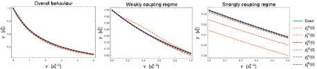
Figure 7. The physical solutions to (61) with approximate  are compared with the exact physical solution yp(0). The function
  corresponds to
  ,
,  to
to  and so on.
Download figure:
Standard image High-resolution image5.5. Comparing all approximations
A comparison between all different approximations is reported in figure 8. For the expansion in ![$ \newcommand{\Wrpa}[1]{\mathcal{W}_{\rm RPA}[#1]} \Wrpa{G_{\rm H}}$](https://content.cld.iop.org/journals/0953-8984/30/13/135602/revision2/cmaaaeabieqn188.gif) we consider a
we consider a  approximated with the first nontrivial two terms after the one prescribed by
  (which are of third and fourth order in
 ![$ \newcommand{\Wrpa}[1]{\mathcal{W}_{\rm RPA}[#1]} \Wrpa{y_{\rm H}}$](https://content.cld.iop.org/journals/0953-8984/30/13/135602/revision2/cmaaaeabieqn191.gif) , the second being identically zero). We also report the second order expansion of yp(0) in
, the second being identically zero). We also report the second order expansion of yp(0) in ![$ \newcommand{\Wrpa}[1]{\mathcal{W}_{\rm RPA}[#1]} \Wrpa{y_0^0}$](https://content.cld.iop.org/journals/0953-8984/30/13/135602/revision2/cmaaaeabieqn192.gif) , which in this model for certain regimes is a better estimate than the expansion of
, which in this model for certain regimes is a better estimate than the expansion of  in
in ![$ \newcommand{\Wrpa}[1]{\mathcal{W}_{\rm RPA}[#1]} \Wrpa{y_{\rm H}}$](https://content.cld.iop.org/journals/0953-8984/30/13/135602/revision2/cmaaaeabieqn194.gif) at lower computational cost, since it involves a lower number of diagrams. For the linearized KBE, we consider the simplest approximation
at lower computational cost, since it involves a lower number of diagrams. For the linearized KBE, we consider the simplest approximation  . We see that the expansion in
 ![$ \newcommand{\Wrpa}[1]{\mathcal{W}_{\rm RPA}[#1]} \Wrpa{G_{\rm H}}$](https://content.cld.iop.org/journals/0953-8984/30/13/135602/revision2/cmaaaeabieqn196.gif) leads to an improvement over
leads to an improvement over  and self-consistent GW. However, in the strongly coupled regime, the best approximation is given by the solution to the linearized KBE
  .
.
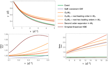
Figure 8. We here compare all approximations to the exact function (42): self-consistent GW, from (50);  starting from GH; next two leading corrections to this latter, according to (56); and, finally, the physical solution to the simplest approximation to the KBE, namely
  from (73). Top panel: overall behavior; bottom panels: ratio between approximate and exact functions in the weak (left) and strong (right) coupling regimes.
Download figure:
Standard image High-resolution image6. Conclusions
We presented two approaches aimed at improving on the GWA outside of the framework set by Hedin in his original formulation. The first one relies on the fact that  can be regarded as the leading order expansion of
  in G0 and
 ![$ \newcommand{\Wrpa}[1]{\mathcal{W}_{\rm RPA}[#1]} \newcommand{\e}{{\rm e}} W_0\equiv \Wrpa{G_0}$](https://content.cld.iop.org/journals/0953-8984/30/13/135602/revision2/cmaaaeabieqn203.gif) . Since there are reasons to believe that W0 may be a better parameter for such a perturbative expansion compared to the bare Coulomb potential vc and even the exact screened one W, we then propose to consider higher order terms in such an expansion.
. Since there are reasons to believe that W0 may be a better parameter for such a perturbative expansion compared to the bare Coulomb potential vc and even the exact screened one W, we then propose to consider higher order terms in such an expansion.
The second approach relies on a Taylor expansion of the Hartree potential in terms of the perturbing potential ![$V_{\rm H}[\varphi]$](https://content.cld.iop.org/journals/0953-8984/30/13/135602/revision2/cmaaaeabieqn204.gif) in the KBE. We consider the hierarchy of linearized KBEs arising by higher and higher order approximations to
in the KBE. We consider the hierarchy of linearized KBEs arising by higher and higher order approximations to ![$V_{\rm H}[\varphi]$](https://content.cld.iop.org/journals/0953-8984/30/13/135602/revision2/cmaaaeabieqn205.gif) .
.
Both schemes have been tested on the one-point model. This is not a 'model system', in the sense of a model for physical systems, but rather as a 'model functional', in the sense of a model for the functionals used in the many-body perturbation theory. The OPM allows to avoid certain theoretical limitations of our current perturbative tools and explore aspects of the theory that would be computationally too demanding to study in real systems. This is a particularly suitable framework for our study, since, as mentioned, there is not a known systematic way to deal with equations such as the KBE. Nonetheless, the procedure we used for the OPM is a necessary proof of principle of the feasibility of the approach and gives leads on how to tackle the full many-body problem.
Results concerning the quality of the approximations in comparison with the OPM equivalent of GWA are encouraging. The series in ![$ \newcommand{\Wrpa}[1]{\mathcal{W}_{\rm RPA}[#1]} \Wrpa{G_0}$](https://content.cld.iop.org/journals/0953-8984/30/13/135602/revision2/cmaaaeabieqn206.gif) seems to be very well behaved and provide good estimates of Green's functions in the strong coupling regimes already with a few orders. This contrasts with the expansion in W, which presents quite an erratic behaviour. The second approach works better, in fact beyond expectations. The solution to even the simplest linearized KBE leads to an approximate Green's function that outperform any other perturbative approach in the strong coupling regime. This suggests that the nonperturbative character of the KBE makes the equation a particularly promising starting point for methods in the strong coupling regime.
seems to be very well behaved and provide good estimates of Green's functions in the strong coupling regimes already with a few orders. This contrasts with the expansion in W, which presents quite an erratic behaviour. The second approach works better, in fact beyond expectations. The solution to even the simplest linearized KBE leads to an approximate Green's function that outperform any other perturbative approach in the strong coupling regime. This suggests that the nonperturbative character of the KBE makes the equation a particularly promising starting point for methods in the strong coupling regime.
For a real system, the first approach presents a theoretically clear path to follow. The way to build the hierarchy of approximations is well defined and, being an expansion in the bare Green's function, there are no problems of spurious solutions. The only limitation is the computational cost of the approach, which is the same as that of an expansion in G0 and vc. The second approach is more sophisticated from a mathematical perspective, but at the same time more clear from a physics point of view: the only approximation is made in the response of the Hartree potential to a perturbing potential. However, the approach is theoretically incomplete, for a lack of mathematical tools for a systematic treatment of the pertinent equations. Our findings in the OPM may give us some guidance, but a complete picture of the procedure for a real system is still to be achieved. Nonetheless, our preliminary tests show such a striking improvement compared with competing perturbative methods that more work in this direction is certainly motivated.
Acknowledgments
The research leading to these results has received funding from the European Research Council under the European Unions Seventh Framework Programme (FP/20072013) / ERC Grant Agreement no. 320971. BSM acknowledges the Laboratoire des Solides Irradiés (Ecole Polytechnique, Palaiseau, France) for the support and hospitality during a sabbatical year. BSM acknowledges partial support from CONACYT-México Grant 153930.
Footnotes
- 5
Such an approximation is the leading order expansion of
![$\delta \bar{G}[\bar{\varphi}]/\delta \bar{\varphi}$](data:image/png;base64,iVBORw0KGgoAAAANSUhEUgAAAAEAAAABCAQAAAC1HAwCAAAAC0lEQVR42mNkYAAAAAYAAjCB0C8AAAAASUVORK5CYII=) which can be obtained combining and both coming from the series that can be derived directly from the KBE (1) by iteration starting from . It is equivalent to the RPA for the irreducible polarizability.
which can be obtained combining and both coming from the series that can be derived directly from the KBE (1) by iteration starting from . It is equivalent to the RPA for the irreducible polarizability. - 6
The entire procedure will be made more clear in the next section, where it will be implemented on a toy model.
- 7
Lani et al considered
but in the OPM with , while Berger et al considered but with V0 self-consistently determined. - 8
We would like to point out that there is strong numerical evidence that these equations, although highly nonlinear, seem to have only one solution, so there is no problem of multiple, spurious solutions at this level.
![$\delta \bar{G}[\bar{\varphi}]/\delta \bar{\varphi}$](https://content.cld.iop.org/journals/0953-8984/30/13/135602/revision2/cmaaaeabieqn064.gif)
![$\delta \bar{G}[\bar{\varphi}]/\delta \bar{\varphi}=G_0 G_0+...$](https://content.cld.iop.org/journals/0953-8984/30/13/135602/revision2/cmaaaeabieqn065.gif)
![$G_0=\bar{G}[\bar{\varphi}]+..., $](https://content.cld.iop.org/journals/0953-8984/30/13/135602/revision2/cmaaaeabieqn066.gif)
![$\bar{G}[\bar{\varphi}]=G_0+G_0 \bar{\varphi} G_0+...$](https://content.cld.iop.org/journals/0953-8984/30/13/135602/revision2/cmaaaeabieqn067.gif)


