

Abstract
The question of which non-interacting Green's function 'best' describes an interacting many-body electronic system is both of fundamental interest as well as of practical importance in describing electronic properties of materials in a realistic manner. Here, we study this question within the framework of Baym–Kadanoff theory, an approach where one locates the stationary point of a total energy functional of the one-particle Green's function in order to find the total ground-state energy as well as all one-particle properties such as the density matrix, chemical potential, or the quasiparticle energy spectrum and quasiparticle wave functions. For the case of the Klein functional, our basic finding is that minimizing the length of the gradient of the total energy functional over non-interacting Green's functions yields a set of self-consistent equations for quasiparticles that is identical to those of the quasiparticle self-consistent GW (QSGW) (van Schilfgaarde et al 2006 Phys. Rev. Lett. 96 226402–4) approach, thereby providing an a priori justification for such an approach to electronic structure calculations. In fact, this result is general, applies to any self-energy operator, and is not restricted to any particular approximation, e.g., the GW approximation for the self-energy. The approach also shows that, when working in the basis of quasiparticle states, solving the diagonal part of the self-consistent Dyson equation is of primary importance while the off-diagonals are of secondary importance, a common observation in the electronic structure literature of self-energy calculations. Finally, numerical tests and analytical arguments show that when the Dyson equation produces multiple quasiparticle solutions corresponding to a single non-interacting state, minimizing the length of the gradient translates into choosing the solution with largest quasiparticle weight.
Export citation and abstract BibTeX RIS
1. Introduction
Single-particle approaches for computing the electronic structure of materials have proven very useful for understanding and predicting the properties of materials, particularly ab initio methods such as density functional theory (DFT) [2, 3]. The local density (LDA) or generalized gradient (GGA) approximations [3–5] for DFT provide practical computational approaches that are the de facto workhorses for obtaining total energies, atomic geometries, vibrational modes, thermodynamic data, chemical properties, kinetic barriers, etc of a great variety of materials. Aside from practical usefulness, the single-particle nature of these approaches permits one to straightforwardly analyze the link between the atomic-scale structure of the material and the resulting electronic structure, e.g., via tight-binding or nearly free-electron models. The relative straightforwardness of a single-particle framework permits one to then propose materials design principles whereby one can tune or engineer desirable materials properties. Nevertheless, there are some shortcomings to such an approach. One can categorize the main drawbacks of single-particle schemes such as DFT for electronic structure predictions into two broad categories.
The first is fundamental to the single-particle approach itself when it is applied to strongly correlated electronic systems. When the basic behavior of electrons is determined by strong and localized electronic repulsions, it is difficult to properly describe such a situation using single-particle approaches where each particle moves separately in an effective potential [6, 7]. A number of methods have been proposed to date to deal with such situations, and at present Dynamical Mean Field Theory [6, 7] represents a workable scheme with the requisite compromise between reasonable computational complexity (obtained by approximating the many-body correlated problem in certain ways) and realistic description of actual materials. Even in such cases, however, building a many-body description of the correlated system for a method such as DMFT requires inclusion of important single-particle terms that reflect the structure, local chemistry and bonding; the strong interactions are added on top of this, as exemplified by the canonical Hubbard model and its various extensions. Thus one needs an 'optimal' single-particle description to begin the process.
A second drawback is due to the ground-state nature of DFT approaches and the use of a local effective potential: even without strong correlations, a theory designed to describe the ground state with a local potential will have a difficult time predicting excited state properties such as band energies and band gaps [8–10]. In a number of cases, one can correct the main faults with self-interaction corrected approaches [4] or explicit inclusion of a degree of Fock exchange in hybrid approaches [11–13]. The popular LDA+U approach [14] falls into this category where Fock-type corrections are included for a subspace of states spanned by pre-chosen localized atomic-like orbitals. The main idea in all these methods is to add more complexity to the effective potential in order to better incorporate the important physics of Fock exchange and to remove the closely related problem of electron self-interaction that plagues the canonical DFT approximations. A more ab initio approach that does not require pre-determined localized basis sets or pre-chosen physical effects is to use the many-body perturbation theory of Green's functions. The most successful to date is the GW approximation to the self-energy [15–19]. The GW approximation delivers high quality band structures of many band insulators and simple metals and automatically includes many physical effects such as exact Fock exchange, localized Coulomb repulsion, dynamic screening, and dispersion forces. In addition, LDA + U is a static and localized approximation to GW [14], and the effective potentials used in hybrid methods generally include a subset of the physics in GW (mainly Fock exchange that is screened in some manner) [11–13]. Most GW calculations are performed perturbatively: they compute corrections to an input DFT-like electronic structure. The final result in turn depends on the input description: in cases where the LDA provides a decent starting point, GW corrections provide a good description of the electronic structure [20–25]. But in other situations, the inadequacy of the input DFT description can create quantitative errors [1, 24, 26, 27].
Ideally, one would like to overcome the starting-point dependence by doing a self-consistent calculation within the GW approach itself. One would aim to have an approach that does not assume any particular basis set or set of parameters. Among many possibilities, two methods have been used by a number of researchers. One is the quasiparticle self-consistent GW (QSGW) [1], and the other is the self-consistent COHSEX (scCOHSEX) [27]. Both move one away from having to use DFT as the starting point for a GW calculation by finding a non-interacting band structure approximately but self-consistently. What this means is that one has a parameter-free method to automatically include static and dynamic screening, Fock exchange, and certain aspects of localized Coulombic physics in a single calculation.
While these methods represent exciting developments, they are based on physical insight and/or approximation of the GW self-energy operator to yield workable schemes. A key question is if there is some theoretical sense in which one can derive an optimal non-interacting band structure for any electronic system, and what such a description would look like. Namely, do these schemes, or various modifications of them, have an a priori theoretical justification?
In this work, we answer this question positively by showing that within the appropriate total-energy scheme appropriate for Green's function methods, namely, the Baym–Kadanoff approach [28, 29] together with the Klein functional [30], quasiparticle self-consistent approaches are the most theoretically justified in the sense that they are 'closest' to the stationary point of the energy functional. The quantitative meaning of closeness is based on gradient minimization, namely the length of the gradient of the energy functional is minimized within the search space considered. Our results thus justify the use of the QSGW approach. We emphasize, however, that our main result is not only applicable to the GW approximation alone but to any self-energy operator. The QS scheme is the optimal one for generating a non-interacting band structure (in the sense of gradient optimization).
The remainder of this paper is organized as follows. Section 2 describes our notation and definitions. Section 3 reviews the Baym–Kadanoff approach specifically within the framework of finding optimal non-interacting band structures. Section 4 describes the small parameter used to organize the gradient optimization process. Section 5 describes how gradient optimization leads to quasiparticle self-consistent equations. Section 6 describes an alternative approach for optimization that one might consider based on optimizing the value of the energy functional itself, but it is shown that this approach, while tempting and easy to state, does not seem to lead to further insights or useful results. Section 7 shows, by numerical solving a simple many-body system as well as by providing more general analytical arguments, that the gradient optimization approach requires choosing the quasiparticle solution with largest weight (Z) when deciding among multiple solutions to the Dyson equation that all correspond to a single non-interacting state. Section 8 has a brief summary of the results and their implications.
2. Definitions and notation
We assume that our electronic system is governed by a time-independent and time-reversal invariant many-body Hamiltonian which means that many key physical quantities such as wave functions are real-valued and all time-dependent quantities depend only on time differences. We use atomic units so  , the unit of elementary charge
  , and the electron mass
  . Hence, energies and frequencies are interchangeable. Wherever sensible, we use matrix notation for compactness. For example, the one-particle electron Green's function for a time-independent system in the frequency ω domain,
  , is a function of three arguments. The x and
  arguments include both spatial coordinates and spin:
  where
where  is a three-vector and
  labels the two spin projections. In matrix notation, we write the matrix
  whose matrix elements are
  .
.
We begin with the non-interacting system. It is specified by the chemical potential μ and the static (frequency-independent) Hermitian single-particle Hamiltonian H0 with orthonormal eigenstates  and real eigenvalues

The unoccupied (conduction) states have  and the occupied (valence) states have
  . For direct comparison to the interacting Green's function and its self-energy, we separate from H0 the part that deals with exchange and correlation
  . We define

Here,  is the electron kinetic energy operator, Uion is the electron-ion interaction potential, the Hartree potential
  is determined by the electron density

via

The static and Hermitian  aims to approximate exchange and correlation effects. In DFT,
  is a local potential. Here, we consider a more general non-local
  ,
,  when
when  .
.
The frequency domain non-interacting Green's function  is given by

We note that for a fixed nuclear configuration and thus fixed Uion,  determines G0 and vice versa. This is a useful parameterization of G0 that we will use below. Finally, the non-interacting one-particle density matrix
  is given by

whose diagonal is the density  .
.
In the frequency domain, the interacting Green's function is given compactly by the Dyson equation

and the self-energy  is frequency-dependent (dynamic) and non-Hermitian and encodes the complex exchange and correlation effects of the many-body system. The Dyson equation can be rewritten as

Therefore, to find the true interacting Green's function, we must replace the static, Hermitian  by the dynamic, non-Hermitian
  .
.
The interacting density matrix ρ is most compactly specified by taking the zero-time value of time-domain Green's function 

Here,  is the Fourier transform of
  and
and  is a negative infinitesimal. This density matrix appears in the expression for the Fock exchange operator.
Finally, for immediate use below, we define two trace operators. For any matrix A, we let  denote the standard definition

Given a matrix that is a function of frequency,  , we define the shorthand
  to stand for the integral

where one can convert the integral to a closed contour integral by going over the upper complex ω plane by using the convergence factor  where
where  is a positive infinitesimal.
3. Baym–Kadanoff approach
The basic point of the approach of Baym and Kadanoff [28, 29] is that both the ground-state total energy and the interacting Green's function  can be obtained by finding the stationary point of an energy functional of G. For simplicity, we concentrate on the Klein functional [30], a functional of both G and the non-interacting G0 given by

where  is the Hartree potential for the electron density corresponding to G0. In the above expression, the frequency dependence of
  and
and  has been suppressed for clarity.
 ![${{E}_{H}}[n]$](https://content.cld.iop.org/journals/0953-8984/29/38/385501/revision2/cmaa7803ieqn044.gif) is the Hartree energy for electron density
is the Hartree energy for electron density  :
:

The functional ![${{ \Phi }_{xc}}[G]$](https://content.cld.iop.org/journals/0953-8984/29/38/385501/revision2/cmaa7803ieqn046.gif) is the exchange-correlation energy functional for the Baym–Kadanoff approach and, as in DFT, is a complicated and unknown functional of G. Formally, it has a well-defined diagrammatic expansion [31]. As in DFT, choosing an approximate form for
is the exchange-correlation energy functional for the Baym–Kadanoff approach and, as in DFT, is a complicated and unknown functional of G. Formally, it has a well-defined diagrammatic expansion [31]. As in DFT, choosing an approximate form for  corresponds to including a certain approximate treatment of exchange-correlation effects. The Klein functional is not the only possible variational functional in Baym–Kadanoff theory: the Luttinger–Ward functional [31] is more widely known, is known to have better variational properties [32] but has a much more complex form. Hence, we will be focusing on the simpler Klein functional.
At the stationary point of F (for both the Klein and Luttinger–Ward forms), the value of F is the ground-state total energy, and the stationary G is the true one-particle Green's function [15, 31]. Unlike DFT, one can obtain, in principle, not just the ground state total energy and electron density but also excited state properties such as quasiparticle wave functions and band energies. Much like the Kohn–Sham DFT approach, there is a functional derivative relation between the exchange-correlation energy functional and the self-energy

To make practical progress in the Baym–Kadanoff framework, two separate types approximations are necessary. The first is the same as that encountered in DFT: one must choose some approximate  . The second challenge is that, unlike DFT where N-presentability conditions are known [33, 34], similar conditions for the Green's function
  are unknown. Namely, one does not know which subset of functions
  correspond to physically realizable Green's functions for the standard interacting electronic many-body Hamiltonian. Therefore, one can try to directly tabulate and work with an arbitrary function
  to locate the stationary point of F, which will hopefully correspond to the physical G, but such an approach is very demanding and computationally expensive. Alternatively, one can make some simplifying assumptions on the types of Green's functions considered.
Here, we restrict ourselves to using non-interacting Green's functions for G. Since it is known that F does not in fact depend on G0 (for fixed G) [35], once we restrict G to be non-interacting, we might as well set G0 equal to G for convenience without any change to F. This also simplifies the functional significantly to

This energy functional contains familiar terms: the noninteracting kinetic, electron-ion, and Hartree energy plus the exchange-correlation contribution. The first three terms are identical to their DFT counterparts and depend only on  . Only
  depends on the added dynamical information in the Green's function G0.
Due to the stationary nature of F about the optimal G, ![$F\left[{{G}_{0}},{{G}_{0}}\right]$](https://content.cld.iop.org/journals/0953-8984/29/38/385501/revision2/cmaa7803ieqn054.gif) provides a variational estimate of the ground-state energy with the error being smallest for the 'best' G0. The main problem, which we have tried to address previously [35] and which we address in this work, is how to choose a best G0 and what this means. A tempting idea is to try to minimize or optimize
provides a variational estimate of the ground-state energy with the error being smallest for the 'best' G0. The main problem, which we have tried to address previously [35] and which we address in this work, is how to choose a best G0 and what this means. A tempting idea is to try to minimize or optimize ![$F\left[{{G}_{0}},{{G}_{0}}\right]$](https://content.cld.iop.org/journals/0953-8984/29/38/385501/revision2/cmaa7803ieqn055.gif) over various trial G0 or equivalently over various trial
over various trial G0 or equivalently over various trial  . However, this program is highly problematic because
 ![$F\left[{{G}_{0}},{{G}_{0}}\right]$](https://content.cld.iop.org/journals/0953-8984/29/38/385501/revision2/cmaa7803ieqn057.gif) does not have any stationary points [35]. Figure 1 illustrates the situation graphically and schematically. The stationary point of F representing the true Green's function that solves the Dyson equation (2) must correspond to a saddle point and to a dynamic and non-Hermitian self-energy, whereas if we constrain ourselves to static and Hermitian self-energies
does not have any stationary points [35]. Figure 1 illustrates the situation graphically and schematically. The stationary point of F representing the true Green's function that solves the Dyson equation (2) must correspond to a saddle point and to a dynamic and non-Hermitian self-energy, whereas if we constrain ourselves to static and Hermitian self-energies  , then F has non-zero derivatives in the whole subspace.

Figure 1. A schematic of the simplest scenario for the Baym–Kadanoff energy functional F. The thick solid lines are level curves of F. The self-energy  that parameterizes the trial Green's function
  is divided into two distinct contributions: a static and Hermitian part
  that parameterizes the non-interacting Green's functions G0, and a remaining dynamical, non-Hermitian part
  . These two independent contributions are high-dimensional matrices but are schematically shown as independent axes. The black circle represents the stationary point of the energy functional which corresponds to the true self-energy that self-consistently solves the Dyson equation (2). The horizontal axis represents the space of all non-interacting Green's functions. We see that the level curves cross this axis with no interruption reflecting the known fact that F has no stationary point when sampled along the horizontal axis [35]. As the figure illustrates, this also implies that the stationary point of F must be a saddle point.
Download figure:
Standard image High-resolution imageWe discuss three avenues for avoiding this pathological situation. The first is to constrain the types of G0 or  being considered based on physical knowledge or intuition. For example, it is known that forcing
  to be a local potential is sufficient to create a minimum for the Klein functional [32, 36, 37]. However, a local potential can not directly and consistently describe a number of simple non-local effects, e.g., Fock exchange which automatically removes problematic electron self-interaction effects. Physically motivated non-local forms for
  are exemplified by the QSGW or scCOHSEX approaches which are based on incorporating GW-level self-energy effects into
  .
.
A second idea is to recast the optimization process by working with a different variable. For example, an interesting recent work [38] shows that, in principle, one can optimize the Baym–Kadanoff energy functional by using the density matrix ρ as the fundamental variable (instead of G) and have a minimum principle for the resulting energy functional. The main difficulty is that one can not avoid the fact that the stationary point of the Baym–Kadanoff functional is a saddle point, so that the optimization process involving ρ still requires an internal search at fixed ρ for a saddle point [38]. To avoid this complexity, an 'NDE2' approximation has been proposed [38] which removes this saddle point search: it basically consists of evaluating  at G0 instead of at G (very similar in spirit to equation (5)). It is our belief that the NDE2 will suffer from this same problems discussed above:
 ![${{ \Phi }_{xc}}\left[{{G}_{0}}\right]$](https://content.cld.iop.org/journals/0953-8984/29/38/385501/revision2/cmaa7803ieqn068.gif) has no lower bound and the minimization will drive the system to an unphysical minimum with negative infinite energy [35]. However, future studies are needed to carefully evaluate this matter. Overall, the density matrix approach to Baym–Kadanoff theory is a promising new idea in the field.
has no lower bound and the minimization will drive the system to an unphysical minimum with negative infinite energy [35]. However, future studies are needed to carefully evaluate this matter. Overall, the density matrix approach to Baym–Kadanoff theory is a promising new idea in the field.
A third approach is to come up with a different mathematical definition of the 'best' G0 which does not rely on naïve optimization of F. We follow this more mathematical approach which will yield a self-consistent quasiparticle scheme. Instead of trying to satisfy the impossible condition  , we will minimize the length of the gradient of F. Specifically, we minimize the square length of the gradient
  where
where  is a trial self-energy. Our results will be general as we will not assume any specific approximation for the self-energy so that the main results will hold for any chosen form of
  . Our approach has similarities to the optimized effect potential (OEP) method [39–41] in DFT. In OEP, one finds the optimal local potential corresponding to the minimum of some general and possibly orbital dependent exchange-correlation energy functional
  : one has a formalism to find the self-consistent local Kohn–Sham potential corresponding to the total energy functional. Hence, both approaches are looking for an optimized and simplified single-particle description (a local potential in OEP and a non-local H0 in Baym–Kadanoff theory). However, whereas in OEP one can find a local potential that minimizes the total energy functional so the functional derivative of the total energy versus the potential is zero, in the Baym–Kadanoff setting one must settle for a non-zero derivative so that the structure and interpretation of the resulting equations for the non-local single-particle Hamiltonian are more complex.
4. Key small parameter γ
As explained above, this paper is focused primarily on the use of non-interacting Green's functions G0. We will be working primarily in frequency space, which is the natural representation when discussing quasiparticle energies and how to deal with the frequency dependence of  . In what follows, we will be employing time-ordered non-interacting Green's functions
  of the following form:

where  . We choose the real-valued quantity
  to be small and fixed. Note that we are choosing to use this class of G0.
In standard textbook treatments [42, 43], one finds the form of equation (6) where the symbol η takes the place of γ, and  is understood or imposed at some point. The quantity η in these standard treatments is a mathematical quantity: an infinitesimal positive that is needed to ensure that Fourier transformations are absolutely convergent when Fourier transforming from time to frequency domain. Often, it is directly included or absorbed into the definition of the Heaviside θ function for the time-ordering operation [43].
In our case, however, γ is positive and small but always finite. We do not send it to zero. It is a fixed number imposed by us manually with a simple physical meaning: it is a damping rate or inverse lifetime for the  energy states. We are giving our non-interacting states in our input Green's function G0 of equation (6) a finite but very small decay rate γ which is equivalent to a very large but finite lifetime
  .
.
Mathematically, we will see that γ acts as a small parameter that (i) regularizes the mathematical expressions we compute by ensuring that they are finite (i.e., avoiding division by zero in energy denominators), and (ii) permits rank-ordering of dominant versus subdominant contributions. Hence, from a mathematical viewpoint, it is necessary to keep γ finite.
However, from a physical viewpoint, the finite value of γ is hardly a restriction. We can take γ to be very small so that the imposed lifetime  can be quite long (a day, a month, a year) and certainly longer than any contemplated experiment which would measure the electronic response. Physically, we need to make γ small enough to resolve and not spoil intrinsic energetic shifts, broadenings and lifetimes stemming from electron interactions and scattering. For example, if the system has a quasiparticle energy gap
  , then
  is required to resolve this gap precisely. Or, if a low-energy quasiparticle state has a lifetime τ due to electron–electron scattering, then
  is needed in order to correctly obtain this lifetime via a calculation of the Green's function. Finally, turning on electron–electron interactions modifies the spectrum of the Green's function (the spectral function) away from its non-interacting analogue. As per equation (2), the energy scale of such changes is determined by the magnitude of the matrix elements of
  , so we require γ to be smaller than these matrix elements to ensure well-converged spectra. This last requirement is directly reflected in the key equations of our analysis below: ratios of matrix elements to γ

appear below and represent the large quantities that must be minimized to obtain the optimal  .
.
5. Shortest gradient of F
In this section, we implement the standard idea of minimizing the length of the gradient vector: the smaller the gradient of F, the closer we should be to the stationary point. Specifically, we seek the optimum non-interacting G0 that delivers the shortest gradient of F.
We begin with the following expression for the variation of F versus G (for fixed G0 and arbitrary G) that is derived by differentiating equation (3):

As a reminder,  . As a matrix derivative, this is equivalent to

Setting this matrix derivative to zero locates the saddle point and automatically yields the Dyson equation (2) for the Green's function.
In what follows, it will be convenient to change variables. Instead of varying G directly, we will vary G via variation of a trial self-energy  :
:

Choosing  to coincide with the self-energy
  that solves the Dyson equation locates the saddle point of F as per equation (7). Matrix differentiation of G gives

Using the cyclicity of the trace, the variation of F is

which corresponds to the matrix derivative

We are interested in the case when G is non-interacting, so we set  and arrive at the simpler derivative

Our objective will be to minimize the squared length of the matrix 

and thereby find a gradient-optimal  and associated G0. The situation is shown schematically in figure 2. Among the set of non-interacting Green's functions parameterized by
  , we are searching for the
  that makes the gradient
  shortest. Figuratively, we have constrained ourselves to be along the horizontal axis of the figure, and we scan along that axis to find the shortest gradient.

Figure 2. Schematic showing the stationary point of ![$F\left[G,{{G}_{0}}\right]$](https://content.cld.iop.org/journals/0953-8984/29/38/385501/revision2/cmaa7803ieqn097.gif) (black circle), level curves of F (solid lines), and the gradient vector
(black circle), level curves of F (solid lines), and the gradient vector  from equation (11) (purple arrows). The axes represent the choices of trial self-energies
  in equation (9) that parameterize the Green's function G. The saddle point corresponds to choosing
  to be the self-energy
  that generates the true Green's function via the Dyson equation. The gradients evaluated along the horizontal axis
  , representing the subspace of non-interacting Green's functions, are
  of equation (12) which are the lowest row of arrows (pointing mainly leftwards). The objective is to find the
  that gives the shortest gradient along the
  axis which in this example is indicated by the dashed circle.
Download figure:
Standard image High-resolution imageWe note that we are not seeking the shortest gradient vector projected into the subspace of non-interacting Green's functions. That would correspond to examining how F changes due to variations  which is different from the much larger set of self-energy variations
  . We are varying the Green's function both along and away from the non-interacting axis and thus in any arbitrary direction. This is indicated in figure 2 by the fact that the arrows representing the gradient have components both along and perpendicular to the horizontal axis.
We aim to minimize  which is the length of the gradient of F versus the trial self-energy
  . As we will see below, it is generally impossible to make the length zero when restricting ourselves to non-interacting Green's functions G0. Hence, the choice of variable for the derivative will, in principle, change the resulting optimum. For example, one could try to minimize
  from equation (8) instead, and one would arrive at a different set of conditions. Therefore, choosing the variable for the derivative requires some physical motivation. Given the choice between
  and
and  ,
,  is a much better choice: choosing G gives useless or nonsense results as detailed in appendix C.
To progress from these graphical ideas to analytic formulae, we calculate the squared norm  in the basis of the orthonormal eigenstates
  by inserting complete sets of states:

Since G0 is diagonal in this basis, this turns into

As expected, this is a sum of strictly positive terms. Our aim is to choose a  so that
  is as small as possible.
We will be using contour integration techniques to evaluate the frequency integral in equation (13). To do this, we need to examine the self-energy  in more detail. Most generally, the self-energy along the real ω axis can be written as a static term plus a sum over poles

where  is the static bare exchange (Fock) operator

The energies  locate the poles of the self-energy which have residues given by the matrices
  . Physically, a pole of
  occurs at an energy where there is strong quasiparticle scattering by electronic excitations, strongly reduced quasiparticle lifetimes, and a strongly damped spectral function. For example, within the GW approximation, these poles correspond to charge fluctuation excitations such as single or multiple electron–hole pairs and plasmons [15, 44]. For a finite system, such as a molecule, the energies
  and associated index a are a discrete and countable set (below the ionization threshold). Above the ionization threshold or in a solid-state system, there are continuous energy bands and thus a continuum of excitations so the sum over a will be an integral and the self-energy will have branch cuts as a function of ω. We note that it is possible to have discrete (bound) states embedded in continuum of states [45], and we will return to these distinctions below when comparing different contributions to the integral of equation (13).
Since  either remains finite or grows sublinearly with ω as
  (see appendix D), and the denominator of equation (13) grows as
  , we can safely turn the integral in equation (13) into a closed contour integral which we choose to go over a half circle at infinity in the upper half plane (the lower half plane gives the same results). Therefore, the quantity we aim to study and minimize is

where

We now perform the contour integral separately for diagonal and off-diagonal contributions to equation (15) since they will scale differently as a function of γ. As a technical aside, we keep in mind that the numerator  in equation (15) begins as a function defined along the real ω axis: when extending it to complex ω, we simply substitute in complex ω into the original functional form (i.e., it is only a function of ω and not of
  ).
).
5.1. Diagonal terms
Consider a diagonal contribution  to equation (15)

There will be two distinct classes of poles contributing to  .
.
The first and obvious one is the pole coming from the zero of the denominator at  in the upper half plane. More precisely, we have

and by using the standard Cauchy integral formula

the contribution from the pole at  is
is

We now series expand in the small parameter γ, and find that the imaginary terms scaling as  cancel as they must since the integral is manifestly positive and real-valued. We end with

and note that the dominant contribution scales as  .
.
The second set of contributions to  will be from poles of
  located above the real axis, i.e., those with
  . The analysis of the contributions from these poles is straightforward but somewhat long-winded and is detailed in appendix A. The result is that the contributions from these poles are subleading: for systems containing discrete energy levels the contributions scale as
  while for systems with only continuous energy bands they scale as
  .
.
All together, we have

where A originates from the pole at  and is proportional to

We focus on reducing the magnitude of the large ratio  to make
  as small as possible since it is dominated by the leading
  term.
term.
In the most general case, the self-energy  will have both real and imaginary parts. By our assumption of time-reversal symmetry,
  and the eigenstates of H0 are real-valued. So we split the matrix element into real and imaginary parts

where

and

Thus the leading term in  is
is

Mathematically, it is unlikely that one can set  since the only free variable is the single real number
  while there are two functions R and I to set to zero. Physically, this corresponds to the fact that
  is Hermitian so it can adjust real-valued energies but never give an imaginary part to the energy which would correspond to a quasiparticle lifetime; such lifetimes are described by non-zero
  . Thus we can set
  by choosing
  while we must settle for a non-zero I in the general case.
Luckily, there are many cases where either  or it is not the main quantity of physical consideration. In systems with discrete energy eigenstates, the lifetimes of excitations will be infinite and thus
  . In solid state systems with continuous energy bands that have an energy gap, quasiparticles whose energies are within one energy gap of either the valence or condition band edges also have infinite lifetimes due to electron–electron interactions since there are no lower-energy states for them to decay into while conserving overall energy. Finally, in most practical GW calculations, one focuses on the real part of
  in order to correct DFT band energies (e.g., [1, 18, 27]). In all these cases, when we choose
  , A becomes zero and this reduces the scaling of
  from
from  to
to  .
.
Summarizing this section, for small γ, choosing the matrix element of  to obey
  is the choice that will make
  as small as possible. For cases where the imaginary part of
  is zero because (i) one has discrete energy spectra, (ii) the system has an energy gap and one is focused on states near the band edges, or (iii) one is ignoring the imaginary part because one is focused on the real part of
  in order to predict band energies, this choice leads to a significant reduction of
  from scaling as
  to scaling as
  . In situations where we also include
  , this choice is the most sensible and obvious. However, the reduction is more modest: the coefficient of the
  scaling is reduced and becomes
  . Either way, this choice requires a self-consistent process because the energy
  and the self-energy
  both depend on
  .
.
5.2. Off-diagonal terms
For a general off-diagonal contribution with 

we have two simple poles above the real ω axis at  and
and  as well as the poles of the numerator stemming from
  . The two simple poles contribute the following term

which scales as  . For the moment, we ignore the additional contributions coming from the poles of
  and instead focus on minimizing the above contribution from the two simple poles. Specifically, our objective is to choose the
  that minimizes the above expression. We envisage this as a self-consistent process where (i) we hold all quantities fixed except for
  which is allowed to vary to optimize the expression, (ii) we update all quantities using the new
  , and (iii) we iterate to convergence.
To simplify the algebra, we define  ,
,  , and
, and  . Keeping in mind that z is real-valued due to our assumption of time-reversal invariance, the expression to be optimized is quadratic in z:

Setting the derivative of this quadratic versus z to zero, we find the optimum

or in other words

This choice is guaranteed to minimize the contributions to  scaling as
  that originate from the simple poles at
  and
and  . For a system with only continuous energy bands, this is a good choice since the contributions coming from the numerator (i.e., the poles of
  ) are subleading and scale as
  as shown in appendix A. However, for a system containing discrete energy levels, the contributions from the poles of the numerator also scale as
  so that the above considerations do not provide an air-tight argument. In appendix E, expressions for these contributions and estimates of their size are provided in the context of optimizing the gradient once self-consistency (QS) is achieved. Whether one should ignore them or include them in the optimization is a subject for future investigation. Finally, as we saw in the case of the diagonal contribution
  , the optimal Hermitian
  is only determined by the real part of
  .
.
5.2.1. Off-diagonal case with degeneracy
The above discussion of the off-diagonal case assumed that  . Specifically, in going from the contour integral of equation (18) to the result of equation (19) it was assumed that
  so that we had two distinct poles contributing. The correct way of proceeding in the case of degeneracy
  is to return to equation (18) and notice that the denominator becomes identical in structure to that of the diagonal case in equation (17). In fact, the only difference with the diagonal case is the replacement of
  by
by  while the remainder of the analysis remains identical. We end up with the optimal choice
  in this degenerate case. It is gratifying that this is identical to the optimal
  in the non-degenerate off-diagonal case where we simply set
  .
.
5.3. Discussion
The main result is that the length of the gradient of the Klein energy functional F is minimized when  is chosen to satisfy

when γ is small.
This choice of  is identical to that of the QSGW method. In QSGW, one approximates the self-energy to its GW form and one sets the imaginary part of the self-energy to zero. The QSGW has successfully described the band structure of a wide variety of solid state systems within the GW approximation for the self-energy [1]. Therefore, in addition to its practical successes, we can say that the QSGW is also mathematically well-founded as it is the choice for
  that minimizes the length of the gradient of the energy functional when approximated within GW. It is 'closest' to the interacting G obeying Dyson's equation.
A critical point of the above derivation is that it is not dependent on the GW approximation itself: the optimum choice of equation (20) holds for any self-energy  at any level of approximation as long as it is derived from some
 ![${{ \Phi }_{xc}}[G]$](https://content.cld.iop.org/journals/0953-8984/29/38/385501/revision2/cmaa7803ieqn208.gif) via
via  . Namely, if we assume that the shortest gradient of the energy functional is best, the recipe of equation (20) is a general answer to the problem of choosing the best non-interacting Green's function to describe an interacting system.
We also note the significant difference between diagonal and off-diagonal elements. Having the diagonal elements obey equation (20) reduces the length of the gradient by factors of  . If the imaginary part of the self-energy is zero or set to zero, then the reduction is very strong: the diagonal contributions in fact become reduced to
  . On the other hand, obeying equation (20) for the off-diagonal elements doesn't actually change the scaling—off-diagonals always contribute
  to the length of the gradient—but it does reduce the magnitude of the coefficients of the terms scaling as
  . Therefore, from a practical point of view, obeying equation (20) for the diagonal elements is of primary importance while obeying it for off-diagonals is of secondary importance. This is a way of rationalizing the observation, dating back to the earliest fully ab initio GW calculations [18], that in many (but not all) cases the most critical corrections to the quasiparticle properties are handled by the diagonal terms of the self-energy.
6. Smallest energy change 

A alternative approach to quantifying which non-interacting Green's function G0 is 'best' is to try to find the G0 that generates the smallest deviation of F from its value at the saddle point. Namely, when scanning along the horizontal axis of figure 1, one looks for the  that generates the G0 so that
 ![$F\left[{{G}_{0}},{{G}_{0}}\right]$](https://content.cld.iop.org/journals/0953-8984/29/38/385501/revision2/cmaa7803ieqn216.gif) is as close as possible to the true total energy
is as close as possible to the true total energy ![$F\left[\bar{G},{{G}_{0}}\right]$](https://content.cld.iop.org/journals/0953-8984/29/38/385501/revision2/cmaa7803ieqn217.gif) where
where  solves the Dyson equation (2). Specifically, what we would like to minimize is the magnitude of the energy difference
  defined as

To make headway analytically, we will assume that the 'best' G0 is sufficiently close to the saddle point so that the difference  or equivalently
  is small enough for a quadratic approximation of F to be accurate. With the quadratic assumption, we can use the general fact that the value of a quadratic function is given by half the dot product of its gradient times the displacement from its stationary point. From equation (10), the gradient of F is
 ![$G\left[{{G}^{-1}}-G_{0}^{-1}+{{ \Sigma }_{xc}}-{{U}_{xc}}\right]G$](https://content.cld.iop.org/journals/0953-8984/29/38/385501/revision2/cmaa7803ieqn222.gif) . The displacement is
. The displacement is  . We are evaluating all these expressions at
  . The situation is graphically illustrated in figure 3. Therefore, the quadratic approximation form for
  is1
is1


Figure 3. Please see the caption of figure 2 for the meaning of the axes, etc. The green vector  represents the deviation of
  from the stationary self-energy
  and connects the saddle point to the chosen
  on the horizontal axis. The dashed circle represents the most desirable
  since at that point the energy F has the same value as it does at the saddle point.
Download figure:
Standard image High-resolution imageAn explicit expression in terms of integrals and matrix elements is

One can proceed by closing the integrals over the upper complex half plane and computing the residues of the integral with separate contributions from the poles in the denominator as well as the poles of  in the numerator. Appendix B contains the details which produce algebraic expressions that do not—for this author—provide insight into how one should proceed.
Aside from the algebraic complexities, there are two other higher level challenges with this approach. First, one is trying to reduce the magnitude of  or equivalently make it as close to zero as possible. However, since we are close to a saddle point,
  will take both positive and negative values which makes the optimization much more challenging than the minimization of a function bounded from below. Second, unlike the previous approach of minimizing the length of the gradient, there is no obvious small parameter such as γ to permit us to perform the optimization process in an organized fashion and to identify the largest terms that must be handled first. Hence, either this smallest-
 -approach is inherently difficult, or a new idea is needed that will take it in a more successful direction. This is an open question.
7. Application of the shortest gradient
In this section, we apply the shortest gradient approach and its associated quasiparticle self-consistent (QS) scheme to understand its behavior in interacting electronic systems. Since this approach justifies practical schemes such as the QSGW [1], the success of QSGW in predicting realistic electronic properties of a wide class of materials may be viewed as an 'application' of the method. Of course, at its best, QSGW is only as accurate as the underlying GW approximation for the self-energy.
We apply the shortest gradient approach to a solvable model many-body system for which we know the exact self-energy. In this way, we can make some conclusions about how this approach and its associated QS scheme describe a many-body system. We focus on a situation where there are multiple quasiparticle solutions corresponding to a single non-interacting state. The existence of multiple solutions is a hallmark of an interacting many-body system, typically with a multi-determinant ground state. A number of realizations of this multiplicity are found in the literature for model systems as well as realistic molecules and materials [46–49].
We study a two-site Hubbard model with a single orbital per site and single electron per site: this Hamiltonian has also been found useful in studying multiple solution situations in prior work [47]. The Hamiltonian is

where  , σ is the spin index, and
  labels the two sites. Due to its simplicity, high symmetry, and small Hilbert space, this Hamiltonian is readily diagonalized by hand for any number of electrons
  . The ground state for
  is a spin singlet. With some minor effort, one can compute the exact one particle Green's functions analytically.
As expected from symmetry considerations and the singlet ground state, the Green's function is diagonal in spin and also diagonal in the basis of bonding (b) and anti-bonding (a) single-particle states,

with non-interacting energy eigenvalues  and
and  (the constant
  is the Hartree potential which we include in the non-interacting eigenvalue as per section 2). The quantity of interest to us is the exact self-energy for exchange and correlation which has two separate forms (bonding and anti-bonding):

Due to the diagonal nature of the problem in the  basis, the shortest gradient is achieved when the QS condition for the self-consistent single-particle
  is satisfied:

Here  , and
, and  labels the two solutions to this equation. The solutions are never at the poles of
  so when solving the above equation we set
  . This can be rewritten as the Dyson equation for the eigenvalue:

Figure 4 shows the usual graphical solution to this equation for weak interaction  and strong interaction
  . For each of a and b, there are two solutions: one solution occurs where the slope of
  is large, and the other solution where the slope is small. Hence, the quasiparticle weights
  for the solutions are small and large, respectively.

Figure 4. Graphical solution to the QS self-consistency condition for the two-site single-orbital Hubbard model at half filling for  (left) and
  (right). An energy solution occurs when the thin blue straight line crosses the thick red curves.
Download figure:
Standard image High-resolution imageFigure 5 shows the evolution of the QS energies and quasiparticle weights as a function of interaction strength  . As expected, for small
  , one set of solutions has Z close to unity with energies evolving smoothly into the non-interacting
  as
as  ; the second set of solutions have very small Z in this limit. For large
  , the system is strongly correlated and does not resemble a single-particle system: all solutions show
  which means that the system becomes impossible to describe with a single Slater determinant. For
  , the QS energies tend to zero or U which are the 'Hubbard bands' for this simple system (the lower and upper Hubbard bands each have half the spectral weight in each a or b channel).

Figure 5. Evolution of the QS energy eigenvalues  and their associated quasiparticle weights
  versus
  for the two-site single-band Hubbard model at half filling. Top panels show Z and bottom panels show
  , and the colors of the curves correspond for a pair of vertical panels (e.g., the large Zb bonding solution in solid blue in the upper left corresponds to the lower energy bonding energy
  in solid blue in the lower left).
Download figure:
Standard image High-resolution imageDue to the existence of multiple (here two) QS solutions for each non-interacting state (b or a), the QS scheme itself does not provide us with a unique solution for the energy states. For each spin channel, any of the four possible combinations of solutions are self-consistent in the QS sense. We now use the criterion of shortest gradient to make a unique choice. We compute the square length of the gradient from equation (13) given by the integral

Due to the high symmetry of the system, in addition to spin degeneracy, the integrals for bonding  and anti-bonding
  have identical values when one uses corresponding solutions (high Z or low Z). Therefore, we omit the spin index and set
  . Furthermore, since the integrals will scale as
  for small γ, we focus on

We numerically evaluate the integrals and tabulate the results in table 1. The table shows that asking for the shortest gradient is a non-ambiguous procedure that clearly favors choosing the large Z solution for any  .
.
Table 1. Scaled squared length of the gradient  for each choice of QS solution associated with quasiparticle weight
  . Values of
  listed in the table are found by first numerically integrating for a set of finite and decreasing values of γ and then extrapolating to
  .
.
 |
 |
 |
 |
 |
|---|---|---|---|---|
| 1 | 0.985 | 1.44 |
0.0149 | 2.74 |
| 4 | 0.854 | 0.185 | 0.146 | 214 |
| 8 | 0.724 | 0.912 | 0.276 | 43.07 |
| 12 | 0.658 | 1.70 | 0.342 | 23.3 |
An order magnitude estimate of the integral for small γ is provided by the linearization  near the QS energy solution, where the term in
  comes from series expansion of
  in γ. The resulting integrals are ratios of simple polynomials and yield
  . However, this underestimates the tabulated value by a factor of two. This estimate has neglected the contribution from the pole of
  which, as explained in section 5, also contributes a term scaling as
  . In this particular model system, the two contributions are equal. Appendix E presents arguments for general cases, beyond this model system, showing that the gradient should be shortest when the solution is chosen that has maximum Z for each non-interacting state.
In this section, we have shown that for systems which present multiple QS solutions corresponding to a single non-interacting state, gradient optimization will choose the solution with largest quasiparticle weight Z. This is sensible since one is asking for the best non-interacting description of an interacting problem, and states with the largest Z are the most non-interacting (i.e., they are the ones best described by a single Slater determinant ground state). This is the best we can do with with a non-interacting description: a non-interacting single-particle Hamiltonian H0 will have one eigenvalue for each eigenvector and can not describe multiple solutions for the same vector. The gradient optimization approach gives a rational basis for choosing solutions with largest Z for each non-interacting state.
8. Summary
The Baym–Kadanoff approach provides a total energy functional of trial one-particle Green's functions that has a stationary point at the physically correct Green's function that solves the Dyson equation. In addition, it provides a recipe for computing the self-energy via differentiation of an exchange-correlation energy functional. In practice, dealing with arbitrary Green's functions is computationally complex and also conceptually difficult as the representability criteria for physical Green's functions are not known. One way forward is to restrict oneself to simpler non-interacting Green's functions.
We have described two approaches to finding the 'best' non-interacting Green's function. The first is based on minimizing the magnitude of the derivative of the Klein energy functional, and this approach produces definite results that form the main body of this paper. The second approach is based on minimizing the error in total energy of the Klein functional between the trial state and the exact state, but this idea needs further development to be useful.
The gradient minimization approach yields a set of equations for the non-interacting Green's function that are identical to those of the quasiparticle self-consistent GW (QSGW) scheme [1]. This means that this type of approach has a firm, a priori foundation. In addition, we have shown that the resulting quasi-particle self-consistent equations are not unique to the GW approximation but hold for any exchange-correlation functional. Namely, the equations are the same for any self-energy in Baym–Kadanoff theory when using the Klein functional.
Separately, by applying the gradient optimization method to a simple but non-trivial many-body system as well as providing more general arguments, we described how this approach chooses the 'best' non-interacting Green's function in cases where there are multiple quasiparticle solutions corresponding to the same non-interacting state. Specifically, gradient optimization favors choosing the solution with largest quasiparticle weight Z: this is intuitively sensible when approximating an interacting system with non-interacting single-particle states since the states with largest Z have the largest non-interacting component.
Finally, not only does our work justify quasiparticle self-consistent schemes, but it also provides theoretical insight and justification as to why a 'diagonal-only' approach for self-energy calculations is a correct starting point and yields good results whereas inclusion of off-diagonal contributions of the self-energy, while physically important in some cases, is of a subdominant nature. Both findings correlate well with practical experience and observations in the field for ab initio predictions of electronic properties.
Acknowledgments
This work has been supported primarily by the National Science Foundation under Grant No. MRSEC DMR 1119826.
Appendix A. Contribution from poles of Σxc
As stated in the text, when performing the contour integral of equation (16), which is reproduced here

a dominant contribution results from the poles above the real axis associated with the denominator at energies  and
and  . The remaining contributions come from the poles of the numerator
  , and in this appendix we examine these poles and the scaling of their contributions to equation (16). We find that the scaling is either
  or
or  depending on whether the spectrum of poles contains discrete states or only continua (bands), respectively.
Taking the matrix element of the self-energy from equation (14) between two states  and
and  , we have

where for compactness we have defined r and sa and suppressed the  indices since we analyze the contribution of a single
  pair.
pair.
The pole energies  can either have a positive imaginary part
  or a negative one
  . A positive imaginary part represents a process moving backwards in time and thus involves holes, while a negative imaginary part means a forward moving process and thus involves electrons. The imaginary part can be larger in magnitude than γ if the associated excitation is physically damped with a significant decay rate
  , but here we take the worst-case scenario for a conservative analysis by setting
  .
.
We split the poles  into the set with positive imaginary part identified with index b and superscript
  and the remaining ones with negative imaginary part identified with index c and superscript
  . We also separate out the real part of the pole energies
  and define them to be
  and
and  . Hence, we have

The main physical assumption we will make on the energies  and
and  is that for any b and c, we always have
  . Disobeying this inequality would mean that a scattering process for electrons (
 excitations which move forward in time) has the same or smaller energy as some other scattering process for holes (
 excitations which move backwards in time) which would imply an electron can scatter into a state below the Fermi energy and/or a hole can scatter into a state above the Fermi energy. In fact, one expects the opposite: an electron scatters into another electron state above the Fermi energy and emits an excitation (positive energy); a hole scatters into another hole state below the Fermi energy minus some excitation (negative energy). For an explicit example, within the GW approximation [50, 51] the inequality is never violated because
  where
where  is an occupied state and
  is some charge excitation such as a plasmon or electron–hole pair while
  where
where  is an unoccupied state and
  is some other charge excitation.
The integral of equation (A.1) has the square of the matrix element, and expanding out the square we have

We note that only a subset of these terms have poles above the real axis. Our task it to find the scaling versus γ of the contributions from such poles to the integral of equation (A.1). To avoid excessively long expressions, we define

The contributions to the integral from the poles of  are
are  times
times

Generally, there is no reason to expect that any of the quasiparticle energies  should precisely equal to any of the excitation energies
  or
or  so that
  and
and  are finite and well behaved as
  . This is rigorously true at low energies for quasiparticle energies close to the Fermi level for a system with an energy gap where the excitations energies
  are greater than or equal to the energy gap. Therefore, the first two terms above are not expected to scale strongly with γ. The third
  and fifth (
 ) terms scale as
  for the case when the double sums are discrete and when the real part of their denominators vanish, while the fourth term
  is finite both by our assumption that
  as well as the fact that the summand is mathematically well behaved as
  . Hence, for discrete sums, the entire contribution has leading scaling behavior
  . For systems supporting continuous energy bands where the b and
  sums are continuous integrals, the scaling of the third and fifth terms is reduced to
  from those bands due to the fact that under an integral

when γ is very small.
In brief, in this appendix we have shown that the contributions to equation (A.1) that stem from the poles of the numerator  generically scale as
  for any discrete poles and as
  if there are only continuous bands of poles in the self energy (i.e., branch cuts).
Appendix B. Energy change ΔF
Here we provide more details for the explicit expression for  in equation (23). For simplicity, let us focus on a single diagonal contribution where
  :
:

The exponential factor in the integrand allows us to turn this into a contour integral by closing the integral contour over the upper complex ω half plane. We then obtain two sets of contributions: residues that originate from the pole at  which only contribute when
  (i.e., n is an occupied state
  ), and residues originating from the poles of
  in the numerator. Inserting the form for
  from equation (A.2) into the above integral and performing the contour integral, one arrives at a first expression

The first contribution for occupied states comes from the pole of the denominator at  while the remaining terms come from the poles of
  at
at  . For unoccupied states
  , only the second set of terms contribute. For occupied states, we can use equation (23) for the first term and perform some algebra to simplify. The final results are for an unoccupied state
  we have

while for an occupied state  we have

Longer expressions with similar structures can be derived for non-diagonal elements  . However, the main problem is that we have no hint as to how to proceed toward minimizing the magnitude of
  based on such expressions.
Appendix C. Unsuitability of minimizing δ F / δ G
We describe the unfavorable consequences of choosing to minimize  instead of
  . The objective is to show that the variable G is a poor choice to generate the derivative whose length we aim to minimize.
Beginning with the expression of equation (7) for  and evaluating it for non-interacting Green's functions
  , we follow the steps in section 5 to find the derivative

the squared length to be minimized

and an explicit expression in the non-interacting eigenbasis

Using the expression for the squared matrix element in equation (A.3) and performing the ω integral, we find

remembering that  is the static part of the matrix element involving the static and nonlocal bare Fock operator
  and
and  .
.
Unlike the situation in the main text where the squared length of the derivative is always finite for any  (i.e., it is a regularized expression since γ acts as an infrared cutoff), the above expression for
  is manifestly infinite and nonsensical unless
  for all choices of
  . The choice
  for all
  means
means  or that our non-interacting G0 must correspond to the Hartree–Fock one regardless of the level of exchange and correlation we decide to include in the exchange-correlation functional
  or the self-energy
  .
.
This is a very poor situation indeed: by choosing to minimize  , we are forced to adopt the Hartree–Fock solution for the non-interacting Green's function G0 not because it necessarily represents an optimum choice but simply to avoid literal infinities in our mathematical description. By contrast, minimizing
  yields finite answers when
  which permits us to proceed in our analysis and find an optimum choice of G0.
Appendix D. Behavior of self-energy as w → ∞
If we assume that equation (14) is true and that the pole energies  are finite, then it is clear that
  is finite and equal to
  . Separately, for such forms of self-energy, any excitation energies such as
  will be finite for a finite physical system solved in a finite basis set.
For the more general case, we can show that  grows at most sublinearly with ω as
  without any assumptions about the functional form of
  . This fact follows directly from the Lehmann representation of the zero-temperature, time-ordered, many-body Green's function for an N-electron system:

where

and  labels the exact many-body eigenstate with M electrons and energy
  where
where  is the ground state. For electron-like excitations
  while for hole-like excitations
  . The electron annihilating field operator is
  . When we send
  , completeness of the eigenbasis and the canonical commutation relation
  lead to

In this limit, one can easily invert the  matrix to find

Comparing this with the Dyson equation (1) shows that  must vanish as
  . Hence, at most,
  grows sublinearly with ω as
  .
.
Appendix E. Choosing largest Z in the multi-pole and multi-band cases
Here we describe analytical results and bounds for optimizing the length of the gradient in situations where there are multiple solutions to the QS equations. Once the self-consistency conditions in equation (20) are obeyed, since we work in the diagonal basis of the non-interaction Hamiltonian H0 determined by this condition, the information content of the non-interacting eigenvalue equation is given by the diagonal QS energy-only Dyson-type equation

For a self-energy given by the form of equation (14), which we write more explicitly here for the case of p poles with real excitation energies  ,
,

the above energy-only QS condition requires finding the roots  of a polynomial of order
  (we are only interested in the real-valued solutions to describe a real-valued non-interacting energy
  ). The question is which of the possible
  solutions has the shortest gradient of the energy functional. We analyze the single-band and multi-band cases separately. We will be assuming time-reversal symmetry and making γ very small to simplify the mathematics.
E.1. Single-band case
Here we only have a single band n to worry about, and the question is which solution  minimizes

where we define the shorthand

and the QS condition means  .
.
One contribution to  for very small γ comes from the pole at
  : near this pole,
  , and plugging this in permits analytical evaluation of the integrals for γ very small (using
  ). The second set of contributions to
  for very small γ come from the poles of the self-energy near
  : for those parts of the integral, the denominator of the integrand is essentially constant and the numerator has a classic Lorentzian form which is easily integrated. We arrive at

Plugging in an explicit form for  gives
gives

If we have a single pole ( ), then both terms are equal and
  so that the solution with smallest
  (i.e., largest Z) will have the smallest gradient.
For multiple poles ( ), we will be assuming that the matrices
  are positive definite and Hermitian (they are such in the GW approximation regardless of whether we use the RPA approximation for W or the exact W [35]). In addition, this is a sensible assumption since it guarantees the diagonal elements of the self energy to have decreasing slopes with ω so quasiparticle weights
  fall in the physical range
  . Thus,
  will be assumed.
Given that  , the above expression for
  has sums of p positive quantities being squared separately or squared after summation, and we can bound the values of the sum. We define a vector
  with p real-valued component
  . Then we can write
  as
as

where  . The first term Pn is the square of the projection
  onto
onto  , and the second term Qn is the Euclidean squared length of
  . If we fix Pn, we are forcing
  to lie on a hyperplane perpendicular to
  . For fixed Pn, the minimum value of Qn occurs when
  is parallel to
  (i.e., all components of
  are equal), in which case
  . For fixed Pn, the maximum value of Qn happens on the extreme corners of the hyperplane in the allowed region
  , which means there is only one non-zero component of
  ; in this case,
  . Since
  , we have the bound

 is clearly controlled directly by
  , so all else being equal, smaller
  gives smaller
  and hence shorter gradients. Specifically, if any two solutions have a ratio of their
  larger than
  , then choosing the smaller
  will definitely lead to a shorter gradient. It is difficult to say much more a priori without knowing more about the distribution of the p components
  .
.
E.2. Multi-band case
For multi-band cases, one must also consider the minimization of off-diagonal contributions  to the length of the gradient for
  . We will be focusing on the non-degenerate case
  since, based on the discussion in the main text, the degenerate case reverts to the diagonal
  case. Reproducing equation (18), we have

For small γ, we have contributions from the two poles in the denominator (see equation (19)) and contributions from the poles of  . Together they give

The QS condition of equation (20) optimizes the first term in the sum above. Plugging in the optimal choice, and then performing some algebraic rearrangements using the fact that  is real by time-reversal invariance, we have

As discussed in the main text, the optimization over  can not help us with the imaginary parts since
  is Hermitian: we are 'stuck' with whatever these values may be. In what follows, we will ignore the contributions from the imaginary part by assuming they are either zero or small. Dropping these terms and plugging in the explicit formula for the self-energy, we arrive at

Our assumptions of time-reversal invariance and zero part of the imaginary part of the self-energy mean that  will be real valued: hence the matrix elements
  are also real valued. Thus we have

To put bounds on this expression, we will require all contributions to be positive inside the squared term for  . Taking absolute values, we have

At this point, we invoke the Cauchy-Schwarz inequality which says that  : this follows from defining an inner product with the matrix
  as the metric, and the positive definiteness of
  leads to this bound. So

where we have reintroduced the vectors  from the previous sections. Viewing the last term as an inner product and applying Cauchy-Schwarz this time to vectors with components
  , we have

where  and Qn were defined in the previous section. Similar logic shows that

Since we know how Pn and Qn are related, we can put an upper bound on  which is

Again, choosing the solution for each state to have the smallest  will ensure
  is as small as possible.
Footnotes
- 1
In practice, we will not know the extremizing
in equation (22) since we are not actually solving the Dyson equation for the extremizing . Instead, if one is using non-interacting Green's function G0, one has access to an approximate self-energy that is evaluated at that G0, namely . However, since we are series expanding about the extremum, the error in is linear in and thus contributes to cubic and higher order terms in so the quadratic expression of equation (22) remains correct at quadratic order.


![$ \Sigma _{xc}^{0}=\delta {{ \Phi }_{xc}}[G]/\delta G{{|}_{G={{G}_{0}}}}$](https://content.cld.iop.org/journals/0953-8984/29/38/385501/revision2/cmaa7803ieqn228.gif)


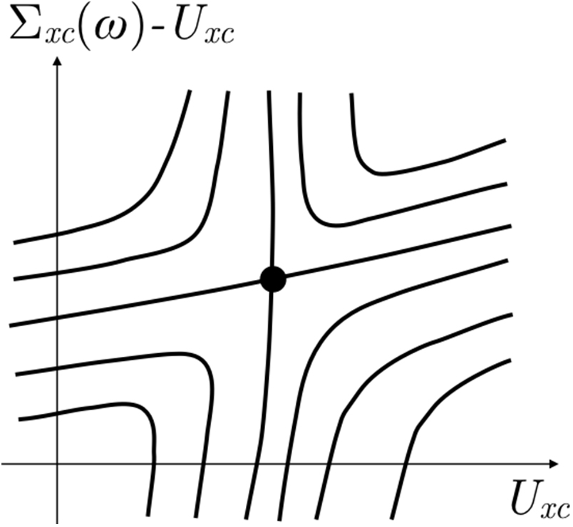
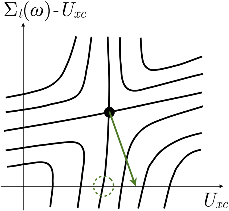
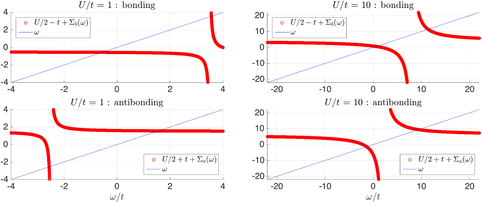
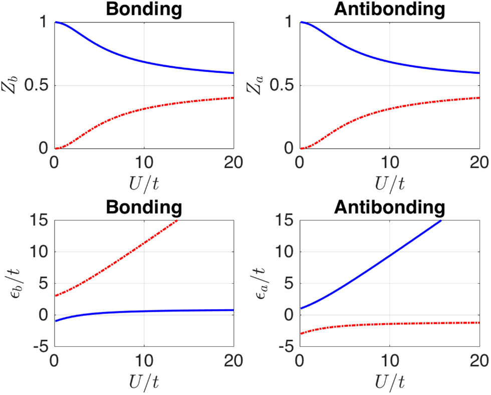