
Abstract
In the past twenty years, hadron spectroscopy has made immense progress. Experimental facilities have observed different multiquark states during these years. There are different models and phenomenological potentials to study the nature of interquark interaction. In this work, we have reviewed different quark potentials and models used in hadron spectroscopy.
Export citation and abstract BibTeX RIS

Original content from this work may be used under the terms of the Creative Commons Attribution 4.0 licence. Any further distribution of this work must maintain attribution to the author(s) and the title of the work, journal citation and DOI.
1. Introduction
Quarks, leptons, and gauge bosons are considered as the most elementary particles observed in laboratories. Due to color confinement, only color singlet configurations of quarks are observed in nature. Mesons and baryons are well-known color singlet structures. Further, Gell-Mann and Zweig gave the idea of color singlet hadronic state with  and
and  quark combinations known as tetraquarks and pentaquarks [1, 2].
Over the past decades, there have been significant advances in experimental facilities. With the help of recent developments in high-energy experiments and computational techniques, many new hadrons are discovered. Recent developments in lattice gauge theory also support experimental results [3–5]. After the discovery of J/Ψ in 1974, heavy quarkonium studies have also become very important in hadron physics [6].
Quantum chromodynamics (QCD) is the theory of strong interaction between quarks and gluons. The study of heavy flavor spectroscopy is important for understanding strong interaction. The fully heavy tetraquark and pentaquark states are perfect prototypes for improving the knowledge of heavy quark potential. A fully heavy tetraquark or pentaquark state involves the non-perturbative color confinement potential and the perturbative one gluon exchange (OGE) interaction [7].
Since interquark interaction is a non-Abelian and non-linear theory, which is very complicated and not understood yet [8]. Therefore, we study interquark interactions with some models. None of the models is capable of explaining all the hadronic systems. The quantum mechanical potential models can reproduce the experimental results for hadron spectroscopy. Potential models are based on the assumption that potential can characterize the interaction between the quark and antiquark. When the quark mass is heavy (mQ ≫ ΛQCD) and the velocity of the quark is v ≪ 1, the system can be treated nonrelativistically, and solving the Schroedinger equation will lead to the properties of the system. For solving the Schroedinger equation of quark–antiquark potentials, there are several analytical techniques. Otherwise, we use relativistic potentials.
In this article, we shall review the quark potentials and models which are extensively used to determine the mass and other properties of hadrons.
2. Quark potentials and models in hadron spectroscopy
There are different methods for hadron spectroscopy to determine the properties of hadrons, it includes the bag model, QCD sum rules, Bethe–Salpeter equation method, various phenomenological potential models, lattice quantum chromodynamics (LQCD), etc. These methods, with some approximations and assumptions are found to be very useful in determining the properties of hadrons.
2.1. The bag model
The two important properties of QCD are asymptotic freedom and quark confinement. The origin and nature of quark confinement are still unknown. One of the very successful phenomenological models for quark confinement is the bag model proposed in 1974 by Chodos et al [9]. The bag model assumes quarks in hadrons are non-interacting and confined in a finite region called 'bag'. The infinite potential of the bag will confine the quarks inside. Quarks can move freely inside the bag and they cannot reach the exterior due to infinite potential.
The general structure of Lagrangian density for MIT bag model is,

where θv is the step function which is zero outside and surface of the bag and unity inside the space-time region of the bag. B is bag constant and Δs is a function that is unity on the bag surface and zero otherwise. The other term is a Lagrange multiplier representing the confinement condition.
The bag model provides the mass and other properties of hadrons in their ground state [10–14]. Chodos et al studied baryon structure in static bag model [10]. The spectrum for low-lying baryon resonances was obtained by assuming the bag as a sphere of constant radius. The Dirac equation was solved by considering quarks as massless. Their study incorporated many successful non-relativistic features of the quark model like magnetic moment and gyromagnetic ratio. The effect of quark-gluon interaction was neglected here.
DeGrand et al studied the light hadrons including baryon octet and decuplet, pseudoscalar and vector meson nonets to get the mass and static parameters using bag model [11]. Unlike the study of Chodos et al [10], quark-gluon interactions were considered this time. Also, non-strange masses were introduced for quarks. The effect of deviation from the spherical shapes of the bags was also discarded. In this work, the number of free parameters was increased to four. Masses of light hadrons for m0 = 0 and m0 = 0.108 GeV (introducing a slight nonstrange mass) were calculated and compared with the experimental values. However, the spectrum was insensitive to the non-strange mass contribution. The theoretical estimation showed good agreement with the experimental results. Authors had also estimated magnetic moments, charge radii, and weak decay constants. Their study also showed that exotic hadrons are unstable. At the end of the study, they proposed the possibility of including charm quark mass to get the charm hadron spectrum.
After the discovery of the charm quark, Jaffe and Kiskis tried to extend this model to get mass spectra of hadrons with charm quarks [15]. They used the cavity approximation to the bag model. Quark-gluon interactions were also taken into account. The mass of hadrons with top (t) and bottom (b) quarks were also proposed (these hadrons were new at that time because t and b quarks were not confirmed by experiment). The study considered baryons with one heavy quark. The mass predicted for  was lower than the experimental result.
Later many improvements were made in the model to get heavy hadron properties. Bernotas and Simonis provided a combined description for light and heavy hadrons (mesons and baryons) in the bag model [16]. The center of mass correction was added to heavy hadrons. It helped to obtain mass spectra that were in good agreement with the experimental values. Their bag model and the MIT bag model have some differences. The zero point energy term (Z0) and self-energy term of MIT bag model were discarded here. The zero point energy term played an important role in the MIT bag model to get a good fit. The number of free parameters was further increased. The values of the mass of hadrons with heavy quarks showed better results than the MIT bag model by Chodos et al [10]. However, results for light hadrons were not much different. Some of the drawbacks of the model were the difference in the π−K mass and Σh −Λh mass splitting. Still, reasonably well results for other hadrons were obtained.
In the MIT bag model combined with chromomagnetic interaction, Zhang, Xu, and Jia calculated the masses and magnetic moments of heavy baryons and tetraquarks with one or two heavy quarks [17]. The results were compared with MIT bag model calculations and experimental results. They have predicted the mass of some states, including the tetraquark state  .
.
As we have observed, the simple formalism of the bag model allows us to represent mesons, baryons, and exotics. Still, the study of exotics in bag model is significantly less.
2.2. Dyson–Schwinger equation (DSE) and Bethe–Salpeter equation (BSE)
Non-perturbative features of quark-gluon propagator can be excellently studied using the Dyson-Schiwnger equation to explain the formation of bound states [18]. Light and chiral quarks are treated equally with heavy quarks in the Dyson–Schwinger–Bethe–Salpeter equation (DSBSE) approach, which creates naturally unified access to both regimes. The approach explained the properties of mesons, baryons, and exotics. The general structure of BSE in case of meson of spin J, total momentum P, and relative momentum k or q can be written as [19],

where Γμ ν⋯(k, P) is the Bethe–Salpeter amplitude, S(p) is the quark propagator, and K is the Bethe–Salpeter kernel. The DSBSE formalism is extensively applied to study baryons and mesons.
Hilger, Rocha, Krassnigg, and Lucha studied open-flavor mesons in the DSBSE approach [20]. They presented the mass and leptonic decay constants. The theoretical studies were compared with the experimental results. The DSBSE approach faces some issues in the case of open-flavor studies which are the pole threshold brought on by complex conjugated eigenvalues, non-monotonic eigenvalues as functions of P2, and non-analyticities of the quark propagators in the complex squared momentum plane.
Hilger, Rocha, and Krassnigg have studied exotic quarkonia of JPC = 1−+ using DSBSE with Rainbow-Ladder (RL) truncation [21]. States with exotic quantum numbers naturally occur in the setting of the quark–antiquark BSE in the DSBSE technique. Masses of the  and
and  were predicted using π1 states as reference. The low-lying state of the charmonium and bottomonium has similar mass compared to the axial vector ground states. It also encourages the study of other quarkonia analogs.
Hilger, Popovici, Rocha, and Krassnigg studied heavy quarkonia using DSE coupled to the BSE equation of mesons with RL truncation [22]. Spectrum for the charmonium and bottomonium systems were reproduced. The results agreed with the observed results.
Same group of authors applied Landau-gauge BSE formalism to the ground and radially excited states of bottomonium using RL truncation in a separate work [23]. A combined result for the ground and excited states of bottomonium is presented with good experimental support. However, two states were out of the description with JPC = 1++ and 1+−. This indicates further degrees of freedom will be mandatory to include these states.
Krasssing and Blank studied the tensor mesons using the DSE equation coupled with the BSE equation of mesons [19]. It was the first covariant study of tensor mesons. The masses were presented as a function of pion masses for tensor, vector, axial vector, scalar, and pseudoscalar mesons. The mass of 2++ state was found to be above all other states across the range from the chiral limit to bottomonium. Also, 2++ states were further explored with RL truncation. Results matched with the experimental study.
Eichmann et al discussed different approaches used to study the spectrum and electromagnetic properties of baryons [24]. They reviewed the success of RL truncation, where interaction between two quarks (qq) got reduced to effective gluon exchange. Also, it was provided with a parameter-free analysis.
Eichmann, Fischer, and Alepuz studied light octet and decuplet baryons in the DS and Faddeev equations using RL truncation [25]. Calculations were carried out using three-body Faddeev equations and diquark-quark approximation. Results for the ground and excited states showed reasonably good agreement between both approaches.
Wallbott, Eichmann, and Fischer studied the X(3872) tetraquark state in DSE formalism [26]. They analyzed two types of quark content, which are  and
and  . Bethe–Salpeter amplitudes were analyzed by three approaches, including hadro-quarkonium, diquark–antidiquark, and heavy–light meson–meson operators. Meson–meson component was found to be dominating in the ground state calculations.
Eichmann, Fischer, and Heupel presented scalar tetraquark solution using BSE [27]. The result explained the light σ mass. The study shows that pion–pion interaction dominates in this case. Masses for κ and a0/f0 were also found. The theory supports the explanation of light scalar nonet as tetraquarks. The analysis also suggested meson–meson component dominates over diquarks-antidiquarks.
Santowsky et al made a generalized BSE approach to tetraquark states [28]. They solved the coupled system of  and
and  . They found that the pion–pion component dominates while the diquark–antidiquark component gives negligible contribution. Diquark correlation inside hadrons is also helpful in DSE [29]. Using continuum Schwinger function methods, diquarks correlations were studied for hadrons. The solution of DSE will be n-point Schiwnger functions of QCD. For pseudoscalar and vector mesons, RL truncated results were stable, indicating that their diquark partners can influence baryons. The authors also suggest that the BSE of diquark is similar to mesons and differs by a factor of 1/2. Therefore, diquark propagators can be found, and diquark mass can be obtained.
Salpeter and Bethe developed BSE formalism aiming an extension to Feynman's formalism of bound state problems involving several particles [30]. The original BSE equation used two-body bound states for the relativistic interaction kernel and related wave functions. The formula effectively calculates the mass spectra of mesons.
Munczek and Jain discussed the properties of  pseudoscalar meson-bound state using the BSE equation coupled with Schwinger–Dyson (SD) equation [31]. They have used the ladder approximation in the Landau-gauge theory. Heavy–heavy, heavy–light, and light–light
  states were studied. The equations were solved to calculate bound state masses, wave functions, and leptonic decay constants. The obtained results and the results from the experiments were in strong agreement. In the case of ladder approximation, the multi-gluon exchange part of the kernel was neglected, leading to limitations such as color gauge invariance and the absence of crossing symmetry. In other work, the same authors have extended their study to obtain the spectrum of vector, scalar, and pseudoscalar meson-bound states with heavy and light quarks [32]. They have simplified the model, assuming that major contribution comes only from one tensor component for a particle with a given spin and parity. The results obtained were similar to the study of Munczek and Jain [31].
Guleria and Bhatnagar have estimated the mass spectrum and leptonic decay constants of heavy–light axial vector mesons (1++ and 1+−) using BSE formalism with ladder approximation [33]. The interaction kernel consisted of confining term and one gluon exchange (OGE) term. The masses agreed with experimental values and results from other methods.
Li, Chang, and Wang used the relativistic Bethe–Salpeter formalism to get the mass spectra and wave functions of bcq baryons [34]. Using diquark formalism with instantaneous approximation, the three-body problem was converted to two two-body problem. The obtained mass spectra of Ξbc and Ωbc were consistent with other studies. The decay properties for these states were not discussed.
Eichmann, Fisher, and Heupel presented the results for ground state tetraquark with JPC = 0++ using four-quark BSE formalism [35]. They used an approximated kernel omitting all the irreducible three-body and four-body interactions. Masses for σ, κ, and a0/f0 were agreeing reasonably well with the experimental results.
Li et al studied fully heavy tetraquark states using BSE formalism [36]. Using instantaneous approximation, the tetraquark state was taken as a bound state of diquark and an antidiquark. The equation was numerically solved to obtain the mass spectra and wave functions. They have used the same model parameters applied for mesons and baryons from Li, Chang, and Wang [34]. The obtained ground state mass spectra for the  was 6.4–6.5 GeV. The comparison with other approaches was roughly consistent with the ground state of
  . Also, obtained masses were lower than the LHCb obtained mass of X(6900) [37]. Therefore, they have proposed that the observed X(6900) may not be the ground state of
  and it may be the first or second radial excited state. They suggest a more detailed study of the inner structure of this tetraquark state. Masses for the ground states of
  were obtained in the range of 19.2–19.3 GeV. The theoretical values of masses from other studies were higher compared to the obtained results.
Abu-Shady, Gerish, and Ahmed studied heavy pentaquarks with JP
values  ,
,  , and
, and  in the framework of spinless Salpeter equation [38]. The pentaquark was considered as an antiquark and two diquarks. In this pentaquark, at least one of the quark is heavy. By choosing the potential energy of quark interaction as a combination of logarithmic potential, linear potential, and spin-dependent potential, they have employed the Bethe–Salpeter equation for pentaquarks. A logarithmic potential was used for the first time here for pentaquarks. The outcome was comparable with other models. The study did not discuss decay properties. One gluon exchange approximation using an instantaneous potential can only be applied to states containing at least one heavy quark. The model parameters were derived using the Cornell and logarithmic potential relationship.
2.3. Chiral quark model
In the limit of vanishing current quark masses, QCD Lagrangian will possess an additional symmetry apart from its color symmetry, the chiral symmetry. Chiral symmetry has a strong association with the current mass of quarks. For the up and down quark systems, chiral symmetry is a good approximation. For other quarks, this is not a good approximation [39]. Chiral symmetry plays an important role in low-energy hadron phenomenology. It has significantly influenced the bag model as the chiral bag model, the chiral quark model, and the cloudy bag model [40].
Skyrme proposed the importance of chiral symmetry and dynamical symmetry breaking [41]. Chodos and Thorn discussed the bag model with chiral symmetry breaking [42]. The bag constant B was the only free parameter. As a result of chiral symmetry, axial current was not conserved at the bag surface. Chodos and Thorn addressed this problem by considering a SU2 × SU2 multiplet (σ, π), which was coupled in a way to conserve the axial current.
The thought of describing baryon as soliton mainly led to the Nambu–Jona-Lasinio (NJL) model, which was one of the most successful models among. The NJL model is a chirally invariant theory related to quark flavor dynamics. NJL model is also called as chiral quark soliton model. The original NJL model has  symmetry by design. When first postulated, it was thought that the pion existed in a massless bound state with the nucleon and the antinucleon [43]. Nambu and Jona tried to develop a chiral invariant quark model for baryons [43, 44]. Here baryons are represented as solitons of certain Lagrangians. The Lagrangian was reduced to a form,

where  is the Goldstone boson field matrix. A wide range of baryon properties, including mass, magnetic moments, mass splitting, and electromagnetic radii, as well as Dirac and Pauli, axial, induced-pseudoscalar, and pion-nucleon form factors, was described by the NJL model due to its simplicity.
Dyakonov and Petrov developed the chiral quark soliton model based on the low-energy QCD [45]. They demonstrated that the dynamical breaking of chiral symmetry may be explained by seeing the QCD vacuum as a diluted medium of instantons. Instantons are non-perturbative gluonic field fluctuations. Quarks can interact by the influence of instantons. Instanton interaction influences the wave functions of nucleons and pions, which causes variations in the up and down quarks' transverse momentum distributions inside a nucleon. Instanton interactions can be independently treated when the spontaneous symmetry breakdown occurs at a distance lesser than the typical radius of hadron [46].
The Skyrme model [41] approaches to χQSM model in the large Nc limit. Skyrme introduced a Lagrangian density by adding non-linear σ -model Lagrangian into it [47].

where e is a dimensionless parameter, U is the field. From the Lagrangian, energy can be calculated, and mass can be obtained. In some cases, the Skyrme Lagrangian also includes symmetry breaking terms. Prediction of a very narrow pentaquark state was always an interesting topic. A narrow pentaquark state by chiral soliton model was initially discussed by Diakonov, Petrov, and Polyakov [48]. Mass and width of Z+ exotic state were found. Praszalowicz studied pentaquaks in Skyrme model [49]. Author has shown that the chiral model also predicts existence of low-lying exotic baryons. They estimated the mass of θ+ pentaquark state. However, θ+ state is not yet confirmed by experiments. Weigel discussed the Skyrme model for the pentaquarks [50] and through calculation they claimed that a narrow pentaquark state in chiral soliton models in S = +1 channel is a myth.
Callan and Klebanov developed a mass relation for strange baryons using this model [47]. With SU(3) symmetry, the strange baryons were treated as the bound state of kaons. The rotation of the skyrmion was ignored to get baryon masses to  . The terms in the kaon field up to the second order were considered and higher order terms were neglected because they represent the self interaction of kaons.
The chiral quark soliton model and Skyrme model has similar group structure. In the large Nc limit, baryons emerge as solitons due to chiral action. This model based on baryons is called the chiral quark soliton model. Yang and Kim derived mass splitting of SU(3) baryons using the chiral quark soliton model by considering the isospin symmetry breaking [51]. They have also developed a model independent approach to derive mass relations. Different mass relations were derived for the baryon decuplet, antidecuplet, and octet. They obtained the Gell-Mann–Okubo mass relation, which agreed well with the experiment. The known experimental results for baryon decuplets determine the unknown model parameters. Masses for Σ* and Ξ* have shown good agreement with the experiment. Compared with the previous studies, the second moment of inertia helped to explain the heavier baryon antidecuplet masses, which were difficult to fix in previous cases. In the present work, authors obtained the masses of baryon antidecuplet and decuplet but did not consider the decay widths.
Fernandez, Valcarce, Straub, and Faessler discussed the quark–quark interaction to study nucleon–nucleon interaction in light of the instanton models [52]. The effective Lagrangian obtained was invariant under chiral transformations. This interaction includes pion and sigma exchanges as non-perturbative components besides the perturbative one gluon exchange. They estimated the nucleon–nucleon phase shift, which agreed with the experimental data.
2.4. Goldstone boson exchange
The spontaneous breaking of continuous global symmetry is connected with the appearance of massless scalar or pseudoscalar particles. These are known as Goldstone bosons.
Glozman and Riska proposed that after chiral symmetry breaking, a baryon can be considered as a three-constituent quark state, where quark interactions are mediated by a central confining term (considered to be the harmonic term) and a chiral interaction term with pseudoscalar mesons as mediators [53–55]. The chiral interaction part is mediated by the octet of pseudoscalar meson and it can be represented as [55],

where  are the Gell-Mann matrices of SU(3) type. The interaction potential behaves like Yukawa potential at long ranges. Whereas it acts like δ function term in the Yukawa interaction for pseudoscalar exchange for short-range.
Glozman, Plessas, Varga, and Wagenbrunn gave a unified description for finding the spectra of light, and strange baryons [56]. The study depended on the Goldstone bosons and constituent quarks arising from the chiral symmetry breaking. The authors found the spectra with the help of a semi-relativistic Hamiltonian and used the variational method for solving. With this formalism, they were able to explain the experimental results.
Later Stancu extended the Goldstone boson exchange (GBE) model to pentaquarks [57]. Stability of  ,
,  , and
, and  , (Q = c, b, t) pentaquarks were discussed. The GBE Hamiltonian was chosen with linear confinement interaction. The Hamiltonian has the form,

For the ground state, positive parity pentaquarks are favored by GBE over negative parity states of the same flavor. Stancu had further studied  pentaquarks using the flavor spin (FS) hyperfine interaction [58]. In order to include the charm quark, it was extended from SU(3) to SU(4) hyperfine interaction. Apart from the Goldstone boson exchange arising from the hidden chiral symmetry, there would be an additional flavor exchange of D/Ds
mesons in presence of a heavy flavor. The SU(4) FS model was used to get the mass of some pentaquark states
pentaquarks using the flavor spin (FS) hyperfine interaction [58]. In order to include the charm quark, it was extended from SU(3) to SU(4) hyperfine interaction. Apart from the Goldstone boson exchange arising from the hidden chiral symmetry, there would be an additional flavor exchange of D/Ds
mesons in presence of a heavy flavor. The SU(4) FS model was used to get the mass of some pentaquark states  ,
,  , and
, and  . Results were compared with the results of LHCb.
Stancu also discussed the stability of multiquark states with heavy quark in the GBE model [59]. Value of ΔE of some tetra and pentaquark states with charm quark was found. Results were compared with the results of OGE. Surprisingly OGE and GBE predicted opposite results. Pentaquarks with strangeness and negative parity were favored by OGE interaction. While the candidates predicted by GBE interaction had positive parity and were non-strange.
Glozman, Papp, and Plessas reported results for some light baryon spectra by rigorous estimation of three-body Faddeev equation [60]. The tensor meson exchanges were neglected. A linear confinement potential with GBE interaction was considered. Masses for the fourteen lowest states in the N and Δ spectra were calculated. Their findings provided more evidence that the GBE is suitable for baryon spectroscopy.
Similarly, doubly charmed pentaquark states  were studied by Yuan, Wei, He, Xu, and Zou [61]. The study used three types of hyperfine interactions, including color-magnetic interaction, chiral interaction (FS), and instanton-induced interaction. Using these interactions, low-lying levels of
  and
and  were found. The model predicted spin parity of both the quark combination as
  for the lowest state. Also, for FS interaction, the lowest state of
  had negative parity, which was contrary to the lowest positive parity state of
  system with one heavy quark.
2.5. QCD sum rules
QCD sum rule is an important non-perturbative method developed by Shifman, Vainshtein, and Zakharov (SVZ) [62]. This is a widely used method in hadron phenomenology. This method is extensively used to get the low-energy parameters of hadrons. In this method, the time-ordered current is expanded into a quark and gluon condensate using operator product expansion (OPE) which can parameterize the long distance attributes of the QCD vacuum. Properties of hadrons can be determined from the current-hadron duality. The method is successfully applied to study the properties of heavy mesons, baryons, and exotics.
Das, Mathur, and Panigrahi investigated the vector meson masses and decay widths using QCD sum rule [63]. The decay properties have been studied for the first time with QCD sum rules. They have used the original sum rule based only on the two-point function of currents given by πμ ν . The πμ ν contains longitudinal and transverse functions. However, only the transverse function was considered here. SVZ derived a rule called the Borel-transformed rule for transverse function. This rule was obtained by keeping only low dimensional terms in the OPE of the two-point function. For masses and decay widths, the experimental value provided the best fit for K* and ϕ. In the case of ρ meson, the calculated width was less than the experimental value. This may arise because the four-quark condensate contribution was significant and errors cannot be neglected. They also found that the results were very sensitive to slight variations in the parameters.
Wang has studied the  and
and 
 heavy baryons [64]. He used the operator product expansion assuming vacuum saturation for higher dimension contribution will be suppressed due to a large denominator. Therefore, the contribution from the higher dimension condensate was neglected in the calculation. Mass of
  was compatible with the experimental value. For
  the value of masses were compatible with other theoretical calculations and lattice QCD values.
Exotic states are also successfully studied using QCD sum rules. Zhang has performed a study of fully heavy pentaquark ( and
and  ) states [65]. As in the usual QCD sum rule, two gluon and three gluon condensates were considered here. Fully charm pentaquark mass is obtained to be
  GeV and for fully bottom pentaquark
  GeV. However, fully heavy pentaquark states are not experimentally detected. They have proposed that this state can be searched through ΩQQQ
ηQ
mass spectrum.
GeV. However, fully heavy pentaquark states are not experimentally detected. They have proposed that this state can be searched through ΩQQQ
ηQ
mass spectrum.
Wang has studied fully heavy hexaquark states using QCD sum rules [66]. However, there is no experimental evidence on hexaquarks. A hexaquark state was considered as three diquarks. They have proposed that the hexaquarks can be searched through the Ωccc and Ωbbb invariant mass spectrum.
In most cases, due to a high degree of accordance with the experimental result, the QCD sum rule prediction is one of the most reliable method for determining unknown properties of hadrons, particularly heavy hadrons. However, the decay properties are not much explored by the QCD sum rule approach.
2.6. Diquark model
The notion of diquarks was initially discussed by Gell-Mann in his original work on quarks [1]. Diquarks were subsequently introduced by Ida and Kobayashi [67] and Lichtenberg and Tassie [68] to characterize a baryon as a composite state of two particles, a quark and a diquark. Lichtenberg and Tassie [68] could not discuss diquarks in detail because of the lack of sufficient experimental data on exotic mesons.
The diquark model plays an important role in hadron spectroscopy. These are considered as the building blocks of exotic hadrons. Diquarks are tightly bound colored objects with two possible SU(3) representations. The direct product of diquark results in a color antitriplet and a color sextet,  .
.
The product of SU(3) matrices contain,

where the first term represents the antisymmetric product with a negative coefficient and the symmetric term has a positive coefficient reflecting the repulsion. Therefore a diquark is assumed to have SU(3) antitriplet with the antidiquark, a color triplet. Jaffe studied the diquark correlation in QCD [69]. It is believed that the diquark correlation can give an answer to some questions in exotic hadron spectroscopy, including the rarity of exotics in QCD. Diquarks are spin 0 or spin 1 system.
In the case of baryons, diquark correlation is useful to apply for bag model, string model, and potential models. For qQQ baryon, the diquark correlation was expected to be perfect because the dynamics necessitate that the mean distance of the q from the center of mass of the QQ pair is much lower than the mean separation of the QQ pair [70]. With the quark-diquark model of a nucleon, Anselmino and Predazzi successfully explained the experimental results [71].
In another work, same authors also discussed the results of the quark-parton model with a symmetry violation in the nucleon sea [72]. However, assuming a diquark-quark picture of the nucleon can rectify the problem. Lichtenberg pointed out that it is possible to incorporate the effects of Pauli's principle by introducing an exchange term in the quark-diquark potential [73].
Jaffe and Wilczek discussed the role of diquarks in exotic spectroscopy for Θ+ pentaquark [74]. This pentaquark was proposed as the combination of two spin-zero ud diquarks and an antiquark. The study differed from the chiral soliton study of Θ+ pentaquark state. This study also suggested that the charm and bottom analog of this state may be stable against strong decays.
Anwar, Feretti, and Santopinto calculated the spectrum of hidden charm tetraquark states  and
and  [75]. The spectrum of tetraquarks was obtained in two steps. Using a relativized quark–quark potential, the diquark masses were obtained. Then tetraquark spectrum was calculated using the relativized diquark–antidiquark potential. The relativistic potential contains one gluon exchange plus confining potential. With
  quark assignment, they obtained tetraquark states X(3872), Zc
(3900), Zc
(4020), Y(4008), Zc
(4240), Y(4260), Y(4360), and Y(4660). With
quark assignment, they obtained tetraquark states X(3872), Zc
(3900), Zc
(4020), Y(4008), Zc
(4240), Y(4260), Y(4360), and Y(4660). With  , they obtained tetraquark states X(4140), Y(4500), and X(4700).
Exotics can be assumed as diquark states and different models can be applied to the system. Some of these are already discussed in the previous and upcoming models.
2.7. String models
The string model is an interesting model in hadron physics [76]. For large interquark separations, QCD perturbation method fails and there is confinement of quarks. Color confinement is an intrinsically non-perturbative phenomenon. The string model is one of the method which explains this behavior. Still, it is not a complete picture.
Mesons are considered as a string of quarks and antiquarks. The site where a quark–antiquark is linked will be a color singlet. When a quark and an antiquark are getting far apart more strings have to be excited to connect the two sites. When the energy is enough to create new hadrons, system breaks and new pair forms [77]. The string has linearly varying energy and constant energy density. This is called the meson string model.

where a is a constant. Carlson, Kogut, and Pandharipande discussed the flux tube model for mesons and baryons [78]. They incorporated the asymptotic freedom and SU(3) flux tube dynamics. The basics of this model come from the Hamiltonian formulation by Kogut and Susskind [79] with the help of lattice gauge theory. The theory requires local gauge invariance. The Hamiltonian, where gluons are represented on a cubic lattice with spatial spacing  is given by,

where E2(l) is the measure of color electric flux, Uij
(l) indicates the color rotation matrix, and UUUU denotes the formation of closed squares by the products of U(l). Several relevant aspects of the long-range behavior of Yang-Mills fields are thought to be described by the strong coupling limit of the lattice gauge theory. Therefore, quarks separated by a large distance get a fluxtube tension  . The form of potential energy which has been stored in the flux tube is deducted as,


where  state has one quark at
  and other quark at
  . The baryon state has three quarks at
  ,
,  ,
,  , each being at an end of a flux tube and at
  the other ends of the three flux tubes meet together. The model also showed that
  was independent of the flavor of the quark. The value was already proposed from the Regge trajectories studies [80] and charmonium spectrum studies [81]. Using this model, spectra of charmonium, bottomonium, mesons with isospin 1, and baryons with isospin 1/2 and 3/2 were found. The authors also studied spectra of ground states, orbital, and radial excitations of charmonium, bottomonium, light mesons, and light baryons [82]. The value of N−Δ splitting was agreeing well with the experiment. For light mesons and baryons, spin–spin splitting and tensor splitting was also agreeing with experimental results. However, this model failed to explain light mesons and P-wave baryon multiplets, spin–orbit splittings by a unified description.
In a separate work, Artru considered a string with quark at one end and an antiquark at the other end for mesons and baryons with three strings joining at a point with quarks at free ends. The study allowed construction of exotic states [83]. The string picture clearly tells the absence of free quarks. Author did not consider the quark spin and quark statistics in this work.
String models of baryons can be q−q − q configuration, three string modes or Y configuration and triangle model or Δ configuration proposed by Sharov [84–86]. The study says the linear string model of baryons is unstable for any value of mass [84]. Sharov has compared the linear string model of baryons with the Y configuration string model of baryons [85]. One drawback of this model was the value predicted for the slope ( ) of the Regge trajectories (
 ) differs from the value of
  of mesons by a factor of 2/3 at large E values.
There are different variants of the string model. Olsson string model approached mesons using various equations like the Bethe–Salpeter equation and generalized Klein–Gordon equation. Goebel, LaCourse, and Olsson explained the Regge trajectories with the help of the string model and showed that varying the quark mass and considering the Coulomb interaction could violate the linear nature of Regge trajectories [87]. The study concludes that when the quarks are massless, both vector and linear confinement results in parallel Regge trajectories. When a potential deviates from linear confinement at small radii, it can result in linear Regge trajectories at higher angular momenta. Another type of string model was given by Soloviev [88]. Here the author had considered a relativistic spinning model of quarks and antiquarks (massive), which led to Regge trajectories of mesons. Current quark masses and string tensions were the main parameters here. The model prediction was compared with the experimentally identified meson masses to get the current quark masses.
2.7.1. Regge trajectories
Regge trajectories of hadrons were introduced by T Regge in 1959 [89, 90]. The mass and angular momentum of hadrons are related by the equation [40],

where n is the principal quantum number and a, b, and c are the slope and intercept parameters. The hadrons lie on a line in the (J, M2) plane called Regge trajectories. Usually, string picture of hadrons is the most popular model used to explain the Regge trajectories. Regge trajectory can be used to obtain the mass spectra of hadrons. As explained earlier in string models by Goebel, LaCourse, Olsson, and Soloviev formation of Regge trajectories was discussed [87, 88].
A study by Semay and Brac used the relativistic flux tube model and obtained a linear Regge trajectory for mesons in the ultra-relativistic limit [91]. The Coulomb-like potential, instanton effect, and constant potential lead to the flux tube picture. The constant potential was taken as a negative value to reproduce the data. The spin effect is added to the potential with the help of the instanton interaction. Here, they assumed the instanton effect acts only for L = 0 meson state. The study showed that the nature of constant potential is important in getting good results. Satisfactory results for many meson spectra were obtained. The constant potential coming from the extremities of the flux tube has given the most satisfying results with theories and experiments.
Sergeenko combined heavy and light quarkonia to develop an analytic expression [92]. Regge trajectories of heavy and light quarkonia in all regions were developed. They used Cornell potential with a constant term. For the square of mass, an analytical equation was developed. The formula incorporates spin–orbit and spin–spin interactions. The interpolating mass formula showed good accuracy in obtaining spectra of bound states of quarkonia.
Ebert, Faustov, and Galkin used the relativistic quark model to study the mass and Regge trajectories of light mesons using a quasipotential [93]. The quasipotential was derived by assuming the resultant interaction was the combination of one gluon exchange with long-range scalar and vector linear confining potential. They were able to calculate masses and the linear Regge trajectories of light mesons.
Nandan and Ranjan investigated the Regge trajectories of pentaquarks with different possible configurations using the flux tube model [94]. Regge trajectories for pentaquarks showed deviation from linear behavior. The result was compared with the available experimental results. At low rotational speed, the mass of pentaquark showed a linear increase, but at the high rotational speed of string, the Regge trajectories became highly nonlinear. They also observed that two different pentaquarks could show the same mass and angular momentum.
It can be clearly seen that more studies are needed in the case of Regge trajectories of exotic candidates.
2.8. Hadroquarkonium model
Dubynskiy and Voloshin developed the hadro-quarkonium model to study the experimental results of heavy–light tetraquarks [95]. This study is inspired by the analogy of hydrogen atom [96]. Surrounding a light matter, a  pair (Q = c, b) forms a hardcore. The light matter will be
  for tetraquarks and qqq for pentaquarks. In another way, a pentaquark can be considered as a baryon-bound state and an excited quarkonium state. The effective Hamiltonian for QCD multipole expansion can be stated as,

where Ei
a
represents a chromoelectric field and  is the chromo polarisability. Eides, Petrov, and Polyakov considered hidden charm pentaquarks as hadro-quarkonium states in a QCD motivated method [97]. They have studied the pentaquark Pc
(4450) [98] as a bound state of
is the chromo polarisability. Eides, Petrov, and Polyakov considered hidden charm pentaquarks as hadro-quarkonium states in a QCD motivated method [97]. They have studied the pentaquark Pc
(4450) [98] as a bound state of  -nucleon. They calculated the decay width for the state, and it agreed with the experimental data. This pentaquark was expected to be one of the hidden charm baryon octet members. Masses for the octet pentaquarks were also calculated. However, the hadro-charmonium approach could not explain the Pc
(4380) pentaquark.
-nucleon. They calculated the decay width for the state, and it agreed with the experimental data. This pentaquark was expected to be one of the hidden charm baryon octet members. Masses for the octet pentaquarks were also calculated. However, the hadro-charmonium approach could not explain the Pc
(4380) pentaquark.
Feretti and Santopinto used hadro-quarkonium formalism to study tetraquarks and pentaquarks with hidden charm and bottom quarks with strangeness [99]. The diquark–antidiquark approach was also used to find the spectrum of hidden charm and bottom tetraquarks. They discussed the possibilities for the formation of  and
and  (n = u, d) as diquark–antidiquark. Their result suggested that strange hadro-quarkonium systems are strongly bound states.
Feretti and group [99] have discussed the tetra as well as pentaquarks' mass calculations for different states while Eides and group [97] have done the calculation for only pentaquark states but they have also estimated the decay properties. Therefore, for pentaquark mass estimation both formulations can be good for comparative studies.
2.9. One pion exchange potential (OPEP)
A nucleon can be considered as a bound state formed due to the exchange of meson, mainly by pion proposed by Yukawa. The long-range pion exchange potential is,

The mechanism of one pion exchange is used to explain the tetraquark with a hidden charm which was able to predict some new tetraquark states [100, 101]. Toernqvist tried to explain some mesonic states which were not fitting with the conventional mesonic  model. He suggested the term 'deuson' for deuteron like meson–meson state [101]. He expected that the pion exchange would play a prominent role here. Toernqvist explained the X(3872) as a
  deuson and they have predicted the masses of these deusons only from pion exchange contribution [102]. The mass of
  with JPC value 1++ and 0−+ were obtained as 3870 MeV, which matched with the X(3872) state. This was experimentally confirmed by Belle later [103].
Eides, Petrov, and Polyakov studied the loosely bound pentaquark in one pion exchange model [97]. The Pc
(4450) pentaquark was considered as a bound state of  . But in this picture Pc
(4380) pentaquark did not give a satisfactory result. They have also found difficulty in explaining the decay of Pc
(4450) pentaquark.
. But in this picture Pc
(4380) pentaquark did not give a satisfactory result. They have also found difficulty in explaining the decay of Pc
(4450) pentaquark.
2.10. Quark pair creation model
The decay of hadrons discusses the creation of quark–antiquark pairs which depends upon QCD. Since there are difficulties in understanding non-perturbative QCD, quark pair creation model is adopted.
2.10.1.
 model or TPZ model

Micu proposed the model that discussed the decays of meson resonance [104]. According to the model, each hadron undergoes a decay that produces a quark pair with the quantum number 0++ from vacuum, which is then mixed with the quark pairs from the parent hadrons to create the daughter hadrons. The model was used to obtain the strong decays of 2+, 1+, and 0+ meson. Later in 1970s, this model was further modified by Orsay group [105, 106]. This model is now extensively applied on hadron strong decays. Following the production of the quark pair, the initial quarks are rearranged to produce an initial mock state. The decay amplitude was obtained by combining the overlap integrals in spin, color, flavor, and orbital spaces for the initial state and the final state.
In a separate work, Feng et al used this model to get the decay width of  mesons [107]. Mass calculated from the Regge trajectories was compared with the experimental mass to identify the possible candidates. Then using
  model decay widths were calculated. One of the two model parameters represents effective radius of the particle. They compared the theoretical values with the experimental values. Mass and width of ρ(1900) and ω(1960) states matched with experimental values. For ϕ(2170), the calculated value and the experimental value for partial and total width showed a mismatch. K*(1410) state also contradicted with the experimental value in both mass and width.
3. Phenomenological potential models
Researchers are investigating several types of potential models to find out the nature of interquark interaction. In heavy quark regime, chiral symmetry is violated and Goldstone boson exchange is also not effective. Therefore, hyperfine splitting cannot be reproduced for heavy mesons. Beyond chiral symmetry, the QCD perturbative effects also come into effect. This can be explained by one gluon exchange (OGE). The OGE potential can have central as well as non-central components.
The non-central OGE term can include spin–orbit, and tensor terms. For point like quarks, the non-central OGE have a 1/r3 term which can be treated perturbatively. Non-perturbative effect, the confinement of quarks, should also be included in any model that attempts to study QCD. Deriving confinement analytically from QCD is still an open challenge. However, lattice QCD studies can provide some support. Therefore, the chiral part of quark–quark interaction potential can be summarised as the combination of central (C), tensor (T), and spin–orbit (SO) potential.

Once the perturbative and non-perturbative effects are considered, quark–quark interaction can also be written as [108],

where V PS is the pseudoscalar exchange potential and V S is the scalar exchange potential.
In the case of heavy quark–antiquark potential (V NR (r)) is a combination of vector and scalar contributions [109],

Apart from the non-relativistic contribution (V NR (r)), interaction potential includes spin-dependent correction (Vspin(r)).

Spin-dependent interactions can cause fine and hyperfine splitting in the mass spectra. The relativistic correction contains spin–spin (H SS ), spin–orbit (H LS ), and tensor (H T ) interactions.

Spin–spin, spin–orbit, and tensor interactions can be incorporated into the potential as,

where S is the total spin and L is total angular momentum.
In hadron spectroscopy, mostly in phenomenological potentials two terms are considered, confinement potentials and hyperfine potentials.
3.1. Confinement potentials
3.1.1. One Gluon Exchange Potential (OGEP)
The OGE model is one of the earliest approaches in hadron spectroscopy discussed by Rujula, Georgi, and Glashow [110], which is the basis of short-range quark interactions. Since all the hadrons are color singlets, the exchange of gluons can bind the quarks inside hadrons. The two-body OGE potential is given by,

where αs
is the running coupling constant. The value of ks
will be −4/3 for  and 2/3 for qq. Since the running coupling constant will decrease as the distance decreases, the potential Vij
will also approach the lowest order as r → 0. Therefore, at short interquark interactions, OGE can be applied.
and 2/3 for qq. Since the running coupling constant will decrease as the distance decreases, the potential Vij
will also approach the lowest order as r → 0. Therefore, at short interquark interactions, OGE can be applied.
The central part of the OGE which contains spin–spin interaction can also be written as [111],

Rujula, Georgi, and Glashow [110] calculated hadron masses by one gluon exchange controlled by a small coupling which was Coulomb-like. The Hamiltonian was of the form,

where L represents the quark binding; p, Q, r, and m represent the momentum, charge, position, and mass of the quark respectively. In the case of two-body Coulomb interaction, Sij includes spin-dependent and tensor terms. They obtained some of the mass relations successfully. Also, some new mass relations were derived in the light of renormalizable gauge field theory that imposed particular interaction and symmetry breaking mechanisms. Some features of the charmed hadron mass spectrum, including the origin of Σ−Λ mass splitting, were also discussed.
Isgur and Karl formulated a quark model framework that studied the spectrum of low-lying baryons with negative parity inspired by QCD [112]. The Hamiltonian was of the form,

and,

The results agreed with the study by Rujula, Georgi, and Glashow [110]. Compared to the study by Rujula, Georgi, and Glashow [110] spin–orbit part of the ansatz was discarded. The results of Σ−Λ mass splitting supported the significance of confining potential in the Hamiltonian. Isgur and Karl also extended their study to low-lying baryons of positive parity [113]. Spin–orbit forces were neglected as earlier. Hamiltonian was again considered as the combination of the hyperfine and confining terms. The findings, which were mostly based on earlier research, agreed well with the attributes of these states.
Isgur and Karl also studied N, Σ, Σ*, Λ, Δ, Ω, Ξ, and Ξ* in their ground state in a similar approach [114] with color hyperfine and flavor independent confinement. Results were in good agreement with the observed masses.
Copley, Isgur, and Karl studied mass and decay rates of baryons with one charm quark [115]. The formulation was similar to previous studies [113, 114]. One of the most important results was the study of stability of  (P-wave) baryon against the strong decay.
3.1.2. The Cornell potential
It is one of the old and extensively used QCD motivated potential developed by the Cornell University group. The potential is mainly used for getting the mass spectrum of heavy quarkonia [123–125]. The potential is a combination of Coulomb and the confining term and has been extensively investigated. These terms may have different functional forms. One of the most extensively used forms of potential is,

where a and b are positive parameters and r is the interquark distance. The potential is quite helpful in addressing the nature of the QCD vacuum, which is paramagnetic and dielectric [126].
Kuchin and Maksimenko obtained an analytical solution for Cornell potential by applying the Nikiforov–Uvarov (NU) method and studied the mass spectrum of charmonium, bottomonium, and Bc
mesons [124]. They modified the variable as  and proposed some approximation scheme in the term
  . They have assumed a characteristic radius r0 for meson, and
  was expanded in a power series around r0 till the second order. This helped to deform the centrifugal potential and this modification was solved by the NU method. The results showed a good agreement with the experimental values and other theoretical values.
Lahkar, Choudhury, and Hazarika used Cornell potential to analyze the mass and decay properties of heavy flavor mesons containing one heavy quark or antiquark with the help of the variational method using Coulomb, Gaussian, and Airy trial wave functions [127]. Properties like mass, decay constant, branching ratios of leptonic decays, and oscillation frequency of heavy mesons were determined. They compared the results with experimental, lattice, and QCD sum rule studies.
Vega and Flores used Cornell potential to describe properties of  ,
,  , and
, and  states [128]. The Schroedinger equation was solved using an approximate method involving variational method and supersymmetric quantum mechanics (SUSY QM). The variational method is an effective tool to get the approximate ground state energies. Supersymmetric QM will help to get the solution of higher energy states. The energy and wave functions of s state of
  ,
,  , and
, and  were obtained. They calculated the energies for the first three states. Approximate wave functions for the ground, first, and second excited states were also provided. The calculated value showed good agreement with the computational value for the ground and first excited states. The decay properties and experimental values agreed equally well.
The charmonium mass spectra and decay properties were presented using Cornell potential by Chaturvedi and Rai [129]. Relative corrections were added to the Cornell and spin-dependent potential terms. They successfully determined the mass spectra and decay properties of charmonium. The Regge trajectories for charmonium states were also determined, which helped to associate some higher excited states with charmonium. Calculated charmonium masses fit the Regge planes perfectly. All the results were compared with experimental results. For 1S and 2S states, the splitting of the energy level was found to be higher than the experimental value. For 3S and 4S states, the results were in better agreement with the results from experiments and other theoretical studies. They have associated the X(3915) and X(3872) as 20 P3 and 21 P3 respectively.
Karliner discussed the heavy baryons spectroscopy with bottom quark [130]. The hyperfine splitting ratio between meson and baryon was estimated with 5 potentials, including Coulomb, harmonic, linear, Cornell, and logarithmic. The coupling strength cancels the ratio between meson and baryon for all potentials with one coupling constant. Masses of ΞQ baryons with quark content Qsd or Qsu was found.
Patel, Shah, and Vinodkumar studied masses of hidden charm tetraquark state  (q ∈ u, d) using Cornell potential [131]. Spin-dependent interactions were added to the potential including spin–orbit, spin–spin, and tensor terms. The model parameters include constituent quark masses and string tension, which were chosen to fit with the ground state masses of experimentally observed X(3823), Zc
(3900), and Zc
(3885) states. The four-body system was considered as two two-body system, with one as a combination of diquark–antidiquark and the other as a cluster of quark–antiquark. Here they assume one quark moves in a static potential of other quarks like the hydrogen atom problem. The tetraquark states X(3823), X(3915), X(4160), Zc
(3900), Zc
(4025), and Ψ(4040) was interpreted as cluster of quark and antiquark. The tetraquark states X(3940), Y(4140), and Zc
(3885) were fitted with the diquark–antidiquark formalism. The X(3940) as diquark–antidiquark with 2++ gives good agreement with experiment and study by Mainani et al [132], whereas Z1(4050) agrees more with the formalism of cluster of quark–antiquark.
(q ∈ u, d) using Cornell potential [131]. Spin-dependent interactions were added to the potential including spin–orbit, spin–spin, and tensor terms. The model parameters include constituent quark masses and string tension, which were chosen to fit with the ground state masses of experimentally observed X(3823), Zc
(3900), and Zc
(3885) states. The four-body system was considered as two two-body system, with one as a combination of diquark–antidiquark and the other as a cluster of quark–antiquark. Here they assume one quark moves in a static potential of other quarks like the hydrogen atom problem. The tetraquark states X(3823), X(3915), X(4160), Zc
(3900), Zc
(4025), and Ψ(4040) was interpreted as cluster of quark and antiquark. The tetraquark states X(3940), Y(4140), and Zc
(3885) were fitted with the diquark–antidiquark formalism. The X(3940) as diquark–antidiquark with 2++ gives good agreement with experiment and study by Mainani et al [132], whereas Z1(4050) agrees more with the formalism of cluster of quark–antiquark.
3.1.3. The Martin potential
Martin potential has the form [133],

where α ∼ 0.1. Their study was motivated by the success of potential models found in the case of heavy quarkonia. The potential generates all the known levels of J/Ψ and ϒ systems studied by Martin previously [134]. One motivation for the study was realising the need for relativistic correction to the heavy quarkonium  and
and  . Inspired by the accuracy of the fit, they considered an assumption that a Fermi-type term is controlling the hyperfine splitting. For
  system 1S, 2S, and 3S states lead to the value of α to be 0.1 with good accuracy. They calculated the masses and relative leptonic decay width of
  ,
,  and
and  . They could only calculate the absolute decay width of ϕ from J/Ψ. The leptonic decay width of ϕ was obtained as 1.6 ± 0.23 KeV and the experimental result for the same was 1.43 ± 0.12 KeV. However, this is accepted because leptonic decay width is sensitive to the wave function and relativistic effects compared to the energy levels. Prediction of masses for these states also agreed with the experimental result.
3.1.4. The Coulomb plus power potential
Patel and Vinodkumar studied the  system using the Coulomb plus power potential
  using different values of ν [135],

This potential is a part of the general form [136, 137],

where α = − 1, β = ν and V0 = 0. The study mainly used the power range 0.1 < ν < 2.0.
Different potential form will result from different ν values. The inappropriate choice of the radial wave function for heavy quarkonia can affect the decay width and spin splitting of J values because both are dependent on the radial wave function of  . Therefore, the value of A was limited as slightly varying according to the principal quantum number n. The Schroedinger equation was solved by the method given by Lucha and Schoeberl [138]. This potential gave the mass spectrum of
  ,
,  , and
, and  mesons up to a few excited states. The excited states with ν = 0.9 to 1.3 agreed with the results from experiments and other theoretical predictions. They also determined the decay constants of 1S to 6S states with and without QCD corrections. Without QCD corrections, the value of the decay constants for
  systems coincides very well with the experimental value, but not for
  systems. For the
  system, a comparison was not possible at that time due to the unavailability of experimental details. The di-gamma and leptonic decay widths were calculated. Di-gamma decay widths agree with experimental values for the range 1.1 to 1.3. However, in the same range leptonic decay widths were overestimated or underestimated with radiative corrections. They expect it may be because the decay occurs at some finite separation, not at zero separation.
3.1.5. Power-law potential
Ciftci and Koru used power-law potential to study the leptonic decay widths and decay constants of mesons [139]. The potential considered was of the form,

where A and ν were greater than zero. Potential parameters were chosen as A = 0.68 GeV, V0 = −0.3961 GeV, and ν = 0.2. When spin–spin and hyperfine interactions were added to the potential they could obtain good results for meson mass spectra.
Richard and Taxil used a set of power-law potential for baryons spectroscopy [140]. They estimated masses of baryons with a heavy quark (qsc and ssc). Three-body problem was solved with the help of hyperspherical harmonic expansion. Results were compared with the experimental findings.
3.1.6. Potential by Jena, Behera, and Panda
They assumed that a quark and antiquark in a meson are confined in a potential of the form [141–143],

where a > 0. The model parameters were a, V0, and nonstrange quark mass. This model considers the spin-dependent forces as perturbation resulting from the one gluon exchange. The effect of the center of mass motion was also considered. They considered the quark-Lagrangian density for this model in zeroth order as,

The mass and decay constant of the pion and the masses of the ρ and ω-mesons were calculated perturbatively. The value of the decay constant agreed with the experimental results.
Later Jena, Behera, and Tripathy extended the study to the radiative transition of light and heavy flavor mesons [143]. Model parameters were preserved as the same. They have included the momentum dependence due to the recoiling of the daughter meson. They found improvement in M1 transition for light mesons. The heavy meson decay width was also comparable with other results.
3.1.7. The Song and Lin potential
Authors proposed a potential for the heavy quarkonium of the form [144],

The potential is a mixture of inverse square root and square root terms. The factors a and b were adjustable parameters. Relativistic effects were also included using spin–orbit and spin–spin terms. The Schroedinger equation was solved using the numerical method. Spin-dependent part of the potential was taken as perturbation. The numerical values for the calculated energy levels of  and
and  did not show much difference when compared with other potential model approaches because r does not vary much. However, it shows clear differences in the case of
  for very small distances (r < 0.1fm). The energy levels of
  ,
,  , and
, and  and the decay rates of
  ,
,  ,
,  , and
, and  were calculated. Most of the results showed improvement compared with experiments and other potential model studies.
3.1.8. The Turin potential
Lichtenberg et al proposed a new phenomenological potential which lies between Cornell and Song–Lin potential [145],

The study by Lichtenberg restricted only to the bottomonium case because it is the least relativistic case among quarkonium. Because a study by Jacobs et al suggests relativistic corrections in bottomonium are minimal [146]. They have included higher energy levels assuming that the higher energy levels can give more knowledge about the long-range part of the potential. However, the decay rates were not considered for the study. They have done a comparative study using different potentials, including Indiana potential (which will be discussed later), Martin potential, Cornell potential, Song–Lin potential, and Turin potential (the name given in [136]). Turin potential was applied for the first time for the quarkonium system. They have assumed that the bottomonium interaction in these static potentials depends only on the distance between the particles (r). The energy levels for bottomonium were calculated using all these potentials. It fitted equally well for Cornell, Song–Lin, and Turin potential when b quark mass varied appropriately and with the vanishing constant term c. They also compared the energy level differences and spin-averaged energy levels for these potentials. They have obtained the χ2 value by fitting the energy differences.
3.1.9. The Harmonic oscillator potential
It is a very important potential in quantum mechanics because it is one of the few quantum mechanical systems for which there is a precise analytical solution. A harmonic oscillator potential takes the form,

where k is force constant. Harmonic oscillator potential is an important term in many of the phenomenological potentials like Killingbeck potential.
Mansour and Gamal chose harmonic oscillator potential with linear and Yukawa potentials to study the mass spectra of quarkonium systems  ,
,  and
and  using Nikiforov–Uvarov method [147]. They have also added the relativistic corrections with spin–spin, spin–orbit, and tensor interactions. The exponential term was expanded by Taylor series up to second order. Their results were in good agreement with experimental data.
3.1.10. The Killingbeck potential
This type potential has the form,

and the potential is known as extended Cornell potential when an inverse quadratic term is added to it.
Abu-Shady et al studied the heavy meson system using the extended Cornell potential [148]. Here the N-dimensional Schroedinger equation was analytically solved by the Nikiforov–Uvarov method for N = 3. The obtained results were applied to  ,
,  ,
,  , and
, and  system to get the mass spectra. The parameters in the model were chosen to fit the experimental data. The energy eigenfunctions and eigenvalues were also obtained in higher dimensional space. For N = 3, heavy meson masses were obtained. The reported results showed well agreement with experimental result. In the case of
  mesons, enough experimental data was not available. In the case of
  mesons 1S, 2S, and 1D states were found close to the experimental value.
Omugbe et al have also studied the non-symmetric extended Cornell potential to get the mass spectra of  ,
,  ,
,  , and
, and  system [149]. The addition of the harmonic oscillator potential and inverse quadratic potential modifies the behavior when r → 0. The problem was solved using the WKB framework. The findings of this study were consistent with those of other analytical techniques and published experimental data.
Salehi investigated ground and excited states of some baryons including N, Δ, Σ, Ξ, Ω using the Killingbeck plus isotonic oscillator potential of the form [150],

The Schroedinger equation was solved numerically to get energy eigenvalues. To obtain the baryon energies and determine the baryon masses, the values were fitted using the parameters of the generalised Gursey-Radicati mass formula. The potential model agreed well with the spectrum of octets and decuplets.
3.1.11. The Polynomial potential
Mansour and Gamal used the polynomial potential to obtain the mass spectra  ,
,  , and Bc
mesons [151]. The mathematical form of the potential is,
, and Bc
mesons [151]. The mathematical form of the potential is,

A special case of this potential used in the study was,

The Schroedinger equation was solved using Nikiforov–Uvarov method to get the energy eigenstates. Here the first term corresponds to Coulomb potential. The term linear in r represents that V(r) is continuously growing as r → ∞ and leads to quark confinement. The third and fourth terms are harmonic and anharmonic terms responsible for quark confinement. The mass spectra for these three states were studied. The study also showed that the harmonic term gives more accuracy to results compared to other potentials.
3.1.12. The Kratzer potential
Another potential form mainly used to study heavy quarkonia is the Kratzer potential. It is an extensively used potential to study molecular structure and interactions. The form of the potential is [152],

In molecular physics this potential is often written as [153],

where a is the internuclear separation and De is the dissociation energy. The study by Bayrak et al presented a method for calculating the solution for non-zero angular momentum state by Kratzer potential using the asymptotic iteration method [154]. Kratzer potential can be combined with other potentials to solve the mass spectra of heavy quarkonia.
Inyang et al used Kratzer potential mixed with the screened Coulomb potential to solve the mass spectra of charmonium and bottomonium states [155]. The series expansion method was used to get the solution. The model parameters for charmonium were calculated by solving the two algebraic equations using the experimental result for the 2S and 2P states. Similarly, experimental value of 1S and 2S states was used for bottomonium. They have applied their results to calculate the masses for 1S, 2S, 1P, 2P, 3S, 4S, 1D, and 2D states. The findings were quite well in agreement with those of the experiments and other theoretical investigations.
3.1.13. Cornell, Gaussian, and inverse square potential
Moazami, Hassanabadi, and Zarrinkamar gave a non-relativistic potential to get the mass spectrum of heavy–light mesons [156]. The proposed potential takes the form

where a, b, c, k0, and α are constants. The model studied the S and P states of B, Bs , D, and Ds mesons. They have solved the Schroedinger equation by considering the inverse square term and Gaussian term as perturbation. The unperturbed part was solved using the Nikiforov–Uvarov method. They have obtained mass spectrum, decay constants, leptonic decay width, and semileptonic decay width for these mesons. The value of mass obtained was compared with other models and most of the values were in good agreement.
3.1.14. The Wisconsin potential
This is a QCD motivated potential. The potential shows perturbative QCD characteristics at a close range and linear confinement characteristics at a far range [157]. The potential has the form,

where Vs
(r) is a short-range potential which is regularized two-loop perturbative potential. VI
(r) is an intermediate potential, which has the form  vanishing for small and large quark separations. VL
(r) = ar is a long-range potential, which represents quark confinement.
vanishing for small and large quark separations. VL
(r) = ar is a long-range potential, which represents quark confinement.
Jacobs, Olsson, and Suchyta proposed a method to get the solution of the Schroedinger and spinless Salpeter equations with QCD inspired Cornell and Wisconsin potential [146]. The potential parameters and quark masses were varied to get good agreement with the experimental data for both Schroedinger and spinless Salpeter equations. They have obtained the charmonium and bottomonium energy levels. The ratios of charmonium and bottomonium energy levels, which were already satisfactory and found to be slightly improved by using relativistic kinetic energy and wave function corrections. The Wisconsin potential showed good results compared to the Cornell potential.
3.1.15. The Yukawa potential or the screened Coulomb potential
There are different forms of exponential type potential. Exponential potentials are important in nuclear physics, including the Woods–Saxon (WS) potential, the generalised WS potential [158], and the Yukawa potential [159]. Yukawa proposed this potential to study the interaction between nucleons. The form of Yukawa potential is,

where α is the screening parameter. This potential was mainly used to get the bound state normalization and energy levels of neutral atoms. Napsuciale and Rodriguez presented an analytical solution to the quantum Yukawa potential [160].
Yukawa potential was combined with linear or other potentials forms and solved for the mass spectra of quarkonia (already discussed in section 3.1.12) [155].
3.1.16. The Morse potential
This type potential has long been used in molecular and nuclear physics to look at the anharmonicities of the vibrational spectra [161]. The Morse barrier potential takes the form,

After a finite distance, the potential gives an asymptotically diverging attraction to the outgoing particle while offering a repulsion to an approaching particle at r < 0.
Jamel studied the heavy quarkonia properties using the trigonometric Rosen–Morse potential [162]. They have considered heavy quarkonia as a system confined in a hard wall potential formed by combining a cotangent and squared cosecant function. The potential of this combination is trigonometric Rosen–Morse potential. The potential was used to examine the state of conformal symmetry in the heavy flavor sector. They have obtained the energy eigenvalues and eigenfunctions with the help of Nikiforov–Uvarov method. These results have been applied to  and
and  quarkonia to obtain the mass spectra and root mean square radii. The results showed satisfactory agreement with the available experimental and theoretical results.
3.1.17. The Hulthen potential
It is one of the short-range potentials in physics [163]. This potential is a modified form of the Eckart potential [164], which has been vastly applied in physics and whose bound state and scattering properties have been studied using different methods. The potential has the form,

where V0 = Ze2 and a is a constant parameter. The Hulthen potential acts like a screened Coulomb potential in short ranges and declines exponentially at large ranges, therefore its bound state capacity is lower than the Coulomb potential.
Akpan et al presented the approximate solutions of the Schroedinger equation with Hulthen-Hellmann potentials for quarkonium systems [165]. The equation was solved by Nikiforov–Uvarov method. The wave functions were obtained in the form of Laguerre polynomials. The study was able to obtain the mass of charmonium and bottomonium states. Quarks were considered to be spinless. The result provides good agreement with the experimental studies and other theoretical studies. A plot of mass spectra with different potential parameters was also presented.
3.1.18. Screened funnel potential
This potential was used for the calculation of  and
and  mesons spectra [166, 167]. The potential has the form,

where μ is the screening parameter. The  is provided to set it apart from non-screening case. The potential will behave like a Coulomb potential at r → 0 and at r → ∞ , it will be
  . The form of the potential is suggested by quenched lattice QCD calculations. The confining part of the potential has the form,

They obtained the masses for low-lying hadrons. The model provided a rather accurate value for the  leptonic decay width, masses, and radiative decays.
3.1.19. The log potential
Quigg and Rosner discussed the potential of the form [168],

with strength C ∼ 3/4 GeV. They showed that quarkonium level spacing becomes independent of quark mass in the non-relativistic limit. They presented features of this potential when it is applied to describe some properties of heavy quarkonium states like energy level spacing and leptonic decay width. They have found that the charmonium system has a denser spectrum than the modified Coulomb potential. They observed that a 4S charmonium level close to 4.25 GeV was essential for the quark–quark interaction for logarithmic potential.
Machacek and Tomozova discussed the energy spectra and leptonic decay width of the Ψ family with the help of either fractional power or logarithmic functions [169]. They used the following potentials,


where A and B were adjustable parameters to produce a good experimental fit. The energy spectrum and leptonic decay widths were obtained. Results showed good agreement with the experimental results. However, the third potential (equation (40) (exhibited more agreement compared to other potentials. For second and third potential, introducing an additional Coulomb term caused the effect of reducing effective quark mass for good results.
3.1.20. Potential by Bhanot and Rudaz
Authors suggested a new potential for the bound states of heavy quarkonium [170]. The idea of new potential came from the thought that neither a solely Coulombic nor a simply linear potential would be sufficient. The suggested potential takes the form

This potential has a logarithmic term that interpolates between a linear portion that confines at long distances and a Coulomb term that is asymptotically free at short distances. The study by Quigg and Rosner showed that a logarithmic potential for the  could give mass splitting independent of quark mass mQ
[168]. Also, the asymptotic freedom of QCD satisfies the Coulombic and linear terms. The independence of 1S−2S splitting on mQ
for
could give mass splitting independent of quark mass mQ
[168]. Also, the asymptotic freedom of QCD satisfies the Coulombic and linear terms. The independence of 1S−2S splitting on mQ
for  suggests a logarithmic part in between. When the three combinations of potentials were selected, the number of model parameters was also increased. They have found that the logarithmic part of this potential has a significant role in finding the properties of J/Ψ. The potential was applied to get the leptonic decay width for the J/Ψ and ϒ family. The results gave excellent agreement on the Ψ spectrum and leptonic decay width. The model could not test for the ϒ leptonic decay width due to the lack of experimental data during that time.
3.1.21. The Indiana potential
Lichtenberg and Wills studied mass spectra of Ψ, ϒ and ζ (bound state of  ) family using a quark–antiquark potential named Indiana potential [171]. The potential has the form,

where α0 and r0 are constants. This is a QCD motivated potential. The need for a logarithmic potential is already discussed by Quigg and Rosner [168] and Machacek and Tomozova [169]. Indiana potential behaves like a weakened logarithmic potential,  at small distances. At large distances, the potential behaves like
  and the weakening of potential is comparable to linear potential. At r = r0 the potential is vanishing. It has one more interesting property,
  , implying that the behavior at large and small distances cannot be adjusted separately. Spin dependence terms were also added to the potential. The wave function was also obtained to get the leptonic decay widths of vector mesons in this family using Van Royen and Weisskopf formula [172]. The results were compared with the experimental data for Ψ and ϒ. The leptonic decay width of Ψ showed a decrease with an increase in mass, which did not agree with the experimental results.
3.1.22. Potential by Celmaster, Georgi, and Machacek
They developed a potential to get s-wave meson masses [173],

![${V}_{{AF}}(r)=\left[\tfrac{-16\pi }{27}\tfrac{1}{\mathrm{ln}\left(\tfrac{1}{{r}^{2}{{\rm{\Lambda }}}^{2}{e}^{2\gamma }}\right)}+O\left(\tfrac{1}{{\mathrm{ln}}^{3}\left(\tfrac{1}{{r}^{2}{{\rm{\Lambda }}}^{2}{e}^{2\gamma }}\right)}\right)\right]\tfrac{1}{r}$](https://content.cld.iop.org/journals/0954-3899/50/7/073001/revision3/jpgacd1a3ieqn143.gif) , where γ is Euler-Mascheroni constant. When
, where γ is Euler-Mascheroni constant. When  , they expect VAF
(r) to dominate. They have also taken into account that energy of the system raises linearly with the increase in separation, Vs
(r) = kr.
, they expect VAF
(r) to dominate. They have also taken into account that energy of the system raises linearly with the increase in separation, Vs
(r) = kr.  was taken as a negligible function compared to the modified Coulombic interaction at short distances and negligible compared to the linear potential at large distances. The hyperfine splitting was taken into account. The parameters in the potential were a, V0, and quark masses. A fit to the s-wave mass spectrum was done by choosing an appropriate quark mass. They demanded that their explanation applies to both light and heavy quark bound states in response to qualitative successes of QCD in describing the light hadron mass spectrum. When they used their model to predict quarks heavier than the charmed quark, the results were qualitatively similar but it was different in detail from those of Eichten and Gottfried's earlier work [174].
3.1.23. Potential by Gupta, Repko, and Suchyta
Authors developed a non-singular potential model to investigate the quarkonium spectra [175]. They have used the semi-relativistic Hamiltonian of the form,

where Vp and Vc are the perturbative and confining potentials. For confining potential they made use of a mixed scalar and vector exchange potential. The form of Vc is given by,

here C1, C2 and C3 are arbitrary constants. They have obtained the energy levels, leptonic decay widths, and E1 transition width. The values agreed well with experimental data of  and reasonably good for
  .
.
3.1.24. The Richardson potential
Richardson proposed a potential incorporating the asymptotic freedom and linear quark confinement of QCD [176]. The potential generates the spectrum of the triplet  and the triplet
  . The form of the potential is,

where the only parameters in the model are scale size Λ and the quark masses. The value of nf
was chosen as three, assuming the effect of heavy quark will be negligible at a distance they were studying. Here the Fourier transform for the coordinate space potential V(r) was taken by considering the one gluon exchange amplitude, which is proportional to  . They have not considered spin-dependent effects on the potential. For ϒ and Ψ systems, experimental results showed a reasonably good agreement with the model.
Bagchi et al used Richardson potential to study energies and magnetic moments of Ω− and Δ++ [177]. They have modified the potential with a new set of scale parameter values for asymptotic freedom and confinement. Moreover, they expect this potential can be a good base for studying the baryon properties.
3.1.25. Klein–Gordon (KG) oscillator potential
Grunfeld and Rocca presented a relativistic confining potential using the Klein–Gordon oscillator to get the mass spectra of  and
and  [178]. The KG oscillator was introduced by Bruce and Minning [179]. This oscillator will behave like a harmonic oscillator (HO) in the non-relativistic limit. The two-body problem was solved to obtain the mass spectra. A KG equation takes the form [179],

where  is a 3 × 3 matrix and ωi
is the oscillator frequency.
is a 3 × 3 matrix and ωi
is the oscillator frequency.

The quark mass and ω are the two free parameters. The quarks were considered as spinless. The results were compared with the Klein–Gordon equation with linear and quadratic potentials [180, 181]. They have also compared their values with a four-dimensional harmonic oscillator model in a quantum relativistic frame [182]. The results have shown a good agreement with the theoretical and experimental data.
3.2. Hyperfine interaction potentials
3.2.1. The chromomagnetic interaction
The hyperfine structure of hadron spectroscopy involves spin-related interaction between quarks or quarks and antiquarks, which have a color factor. The color-magnetic interaction that results in the mass splitting for ordinary hadrons is caused by the one gluon exchange potential. The Hamiltonian of the color-magnetic interaction, often known as the chromomagnetic interaction (CMI) model is an efficient way to describe hadron masses after the quark mass is included [116].
There are many types of CMI Hamiltonian. The general structure of the Hamiltonian for the CMI model is,

where mi is the effective mass, vij is the coupling parameter, and λi is the Gell-Mann matrices. CMI models contain coupling coefficients and effective masses as parameters. In a simple CMI model the coupling constant and effective quark mass can be extracted from known hadrons.
In the case of doubly heavy baryons the experimental studies are very few but its theoretical studies are done extensively. Weng, Chen, and Deng studied the masses of doubly heavy and triply heavy baryons using the chromomagnetic model with color interaction [117]. In 2017 LHCb reported the doubly charm  state [118]. The calculated value of Ξcc
by this study was close to the LHCb result. For getting the model parameters (mqq
and vqq
) of baryons, experimental data of the light and singly heavy baryons were used. They had extracted thirteen model parameters. The study did not discuss the decay properties.
state [118]. The calculated value of Ξcc
by this study was close to the LHCb result. For getting the model parameters (mqq
and vqq
) of baryons, experimental data of the light and singly heavy baryons were used. They had extracted thirteen model parameters. The study did not discuss the decay properties.
Guo et al studied mass spectra of multi-heavy baryons and S-wave doubly heavy tetraquark  (Q = c, b, q = u, d, s) with JP
= 0+, 1+, and 2+ in the improved CMI (ICMI) model, which includes chromomagnetic and chromoelectric interactions [119]. The parameters (mij
and vij
) were extracted by fitting it with the conventional hadron spectra. Their study included doubly and triply heavy baryons. The study also proposed the mass of Ξcc
baryon. The study gave similar result compared with the study by Weng [117]. However, they were able to predict the masses of tetraquark states also. The predicted mass of
(Q = c, b, q = u, d, s) with JP
= 0+, 1+, and 2+ in the improved CMI (ICMI) model, which includes chromomagnetic and chromoelectric interactions [119]. The parameters (mij
and vij
) were extracted by fitting it with the conventional hadron spectra. Their study included doubly and triply heavy baryons. The study also proposed the mass of Ξcc
baryon. The study gave similar result compared with the study by Weng [117]. However, they were able to predict the masses of tetraquark states also. The predicted mass of  tetraquark state agrees with the LHCb results. The mass of tetraquark states
  ,
,  ,
,  ,
,  ,
,  , and
, and  (n = u, d) were also predicted.
Chen et al used the simple chromomagnetic interaction model to study the triply heavy ( ) tetraquark states [120]. They have used a diquark–antidiquark
 ![$[({QQ})(\bar{Q}\bar{q})]$](https://content.cld.iop.org/journals/0954-3899/50/7/073001/revision3/jpgacd1a3ieqn164.gif) approach and a triquark–antiquark
approach and a triquark–antiquark ![$[({QQ}\bar{Q})(\bar{q})]$](https://content.cld.iop.org/journals/0954-3899/50/7/073001/revision3/jpgacd1a3ieqn165.gif) approach. Both methods gave same results. However, this approach could not predict the masses accurately. The reason comes from the effective coupling constant. Therefore, they suggested an improved model with color-Coulomb term, kinetic term, and confinement term instead of this simple model. They also predicted the decay properties of the states.
approach. Both methods gave same results. However, this approach could not predict the masses accurately. The reason comes from the effective coupling constant. Therefore, they suggested an improved model with color-Coulomb term, kinetic term, and confinement term instead of this simple model. They also predicted the decay properties of the states.
Heavy flavor pentaquark states are also studied using CMI models with chromomagnetic and chromoelectric contributions. An et al studied the mass spectra of heavy pentaquarks with four heavy quarks ( ) [121]. They calculated the relative partial decay width of
  and
and  pentaquark states. However, this type of pentaquark is not identified by any experiment till now. Therefore, more investigation on this type of pentaquarks states is necessary to identify its exotic nature and other properties. An et al extended their study to the fully heavy pentaquark states using the same formalism [122]. After the systematic calculation of the CMI Hamiltonian, mass spectra of
  were calculated.
3.2.2. Potential by Bhaduri, Cohler, and Nogami
They proposed a non-relativistic potential for mesons [183]. The meson spectra were generated initially to get the ground state masses of baryons. It was assumed that the strength of qq interaction was half of  interaction. The potential was of the form,

Spin–orbit and tensor terms were neglected. They calculated the ground state baryon mass with S = 1/2 and S = 3/2. Later Brac used this potential for baryons with more than one heavy quark [184]. Faddeev equations were used for solving the three-body problem. Calculations were performed for static parameters, like wave functions at the origin and mass, charge, and magnetic radii. A harmonic oscillator basis with states up to 8 quanta is used to calculate the spectrum for each baryon.
3.2.3. Potential by Halzen
The author presented a phenomenological non-relativistic quark–antiquark potential in the center of mass system. The potential has the form [185],

where Vc (r) is a spherically symmetric infinite potential hole of radius a,

here the spin-dependent terms were considered as perturbation. The energy eigenvalues were given by the zero point Bessel function. They have obtained the energy eigenvalues for L = 0 and L = 1 states. The model was also able to predict the D wave boson masses. They have also observed that for a = 1/1.33mπ and Mq = 5 GeV/c2 many other physical properties of mesons can be derived.
3.3. Potential with confinement and hyperfine interactions
3.3.1. Potential for by Weinstein and Isgur

Weinstein and Isgur considered a non-relativistic potential model for tetraquarks [186]. This system was already studied with the help of the bag model and other relativistic potential models. Those studies concluded that dense discrete spectra exist for these states. Apart from previous potential model studies which were not considering the long-range color mixing effects, color confinement forces, and hyperfine interactions were considered here. They have solved the four-particle Schroedinger equation. The Hamiltonian was considered as,

where Hconf is harmonic confinement potential and Hhyp is color hyperfine interaction. The Hamiltonian did not consider the anharmonicities, the effect of possible  annihilations via gluons, and some relatively small spin–orbit and tensor effects. The model did not give evidence for any denser discrete spectrum for the states. The model confirmed that light
  states can exist with 0++. Also, it allowed the existence of meson–meson-bound states like the nucleon–nucleon interaction of deuteron.
4. Lattice QCD (LQCD)
At high energies, perturbation theory can be used to get the analytical solutions of QCD. However, the perturbation method fails at lower energies. Therefore, an alternative approach, the LQCD is used to calculate the QCD predictions numerically. The domain in which the perturbation method fails, LQCD provides a nonperturbative tool for finding the hadron spectrum and the matrix elements. LQCD is developed on a discrete Euclidean space-time grid and retains the fundamental characters of QCD. Field theory is applied to LQCD via the Feynman path integral method. Numerical simulations of LQCD use Monte-Carlo integration of the Euclidean path integral [187].
LQCD has two applications. Lattice regularisation acts as a non-perturbative regularisation scheme and can be used to perform any typical perturbative calculations. Second, using methods similar to those utilized in statistical mechanics systems, it is possible to simulate LQCD on a computer by converting QCD into a space-time lattice. The correlation functions of hadronic operators and matrix elements of any operator between hadronic states can be calculated using these simulations in terms of the fundamental quark and gluon degrees of freedom. The chiral symmetry breaking, equilibrium properties, and confinement mechanisms of QCD at finite temperatures can also be addressed by LQCD. It offers a useful function where the input settings can be fixed. Therefore, it is possible to estimate quark masses and the strong coupling constant αs . These facts can be utilised to constrain theories like phenomenological models, heavy quark effective theory, and chiral perturbation theory. Testing QCD theories and processes with significant momentum transfers is the primary aim of LQCD.
LQCD studies are helpful in getting new hadron states. Tetraquark states X(3872) [188], Y(4260) [189], the charged Zc
states [190], the doubly heavy tetraquark states [191], and the hidden charm pentaquark states [192] were studied with the help of LQCD. The mass spectra of the tetraquark state Y(4260) were studied in quenched lattice QCD with exact chiral symmetry [193]. The mass spectra of hybrid charmonium ( ), molecular operator, and diquark–antidiquark operators were computed. It has also suggested a possibility that Y(4260) can be an excited state of
  .
.
Brambilla, Consoli, and Prosperi gave a derivation for the quark–antiquark potential in a Wilson-loop context [194]. The basic assumptions, the condition used for the validity of potential and the relation with the flux tube model were considered in the Wilson-loop approach. The potential contains three terms One is a static term (stat), the spin-dependent term (SD) and the velocity-dependent term (VD),

The same approach was extended to get the three quark potential,

They have presented the form of each term. In the case of three quark potential, they have observed that the short-range part of the equation for the three quark potential was a pure two-body type potential. This can be compared with the electromagnetic potential for three charges. The spin-dependent term contains a long-range part which was coinciding with the expression given by Ford as [195],

The spin-dependent potential for three quark has been consistent with the Wilson-loop context. The order 1/m2 for qqq potential was also new to their study. They have done spin-independent relativistic correction on  and qqq. This way, better results were obtained by assuming scalar confinement.
Bicudo et al gave a theoretical method to get the mass and decay width of doubly heavy tetraquark  [196]. The potential between two heavy antiquarks
 ![$[\bar{Q}\bar{Q}]$](https://content.cld.iop.org/journals/0954-3899/50/7/073001/revision3/jpgacd1a3ieqn178.gif) and two light quarks [qq] was parametrized by a screened Coulomb potential using lattice QCD,
and two light quarks [qq] was parametrized by a screened Coulomb potential using lattice QCD,

where α and d were parameters dependent on isospin and angular momentum of qq pair. The Schroedinger equation was solved for the potential to obtain mass and decay width. Mass for the state was obtained as m = 10576 ± 4 MeV and  MeV.
MeV.
5. Summary and outlook
From the above review, we have seen that hadron spectroscopy can be studied by many methods. In this article, we have classified them on models and potentials.
Table 1 shows the list of different models we have reviewed and particles studied in these models. BSE formalism, CMI method, and QCD sum rules have studied fully heavy pentaquarks. However, such type of system is yet to be detected experimentally. In BSE and CMI models fully heavy tetraquarks are studied. Doubly heavy and triply heavy tetraquarks are also discussed in different models successfully. Such tetraquarks have been observed recently also. We expect that this work will be helpful in explaining these data. QCD sum rule is also found to be helpful in the study of hexaquarks. Unfortunately, most of the studies are devoted to mass calculations, only a few studies have investigated the decay properties.
Table 1. Different models and the system studied in that model.
| Model | System studied |
|---|---|
| Bag model |
 , qqq, , qqq, 
|
| OGE | light and heavy baryons and heavy flavour tetraquarks and pentaquarks |
| GBE | light and heavy baryons and heavy flavour tetraquarks and pentaquarks |
| BSE |
 , ,  , ,  , bcq, , bcq,  , , 
|
| CMI |
QQq, QQQ,  , ,  , , 
|
| QCD sum rule |
 , QQq, , QQq,  , QQQQQQ , QQQQQQ
|
| Diquarks |
 , , 
|
| Skyrme model | qqq |
| Hadroquarkoium |
 , , 
|
| OPEP | Pc pentaquark |
The CMI Hamiltonian is useful in determining the mass and decay properties of fully heavy pentaquarks. However, the determination of parameters, mi and vij in the CMI Hamiltonian is difficult due to the lack of sufficient experimental data. As we have observed, some models consider exotics as diquarks. It is expected that the diquark correlation can answer some puzzles in exotic hadron spectroscopy, including the rarity of exotics in QCD.
We have plotted the form of five phenomenological potentials (Cornell, polynomial, Kratzer–Yukawa, Cornell–Gaussian-inverse square, and Hulthen–Hellman) given in figure 1. The mathematical form of these potentials is given in table 2. Apart from these, Coulomb potential, harmonic potential, and Yukawa potential are also included in the plot. All the potentials are used to get the mass spectra of heavy quarkonia ( and
and  ). Cornell potential and combination of Cornell, Gaussian, and inverse square potentials show almost same behavior after 2fm separation. Hulthen–Hellman potential shows a large deviation from other potentials. However, potential approaches to other potential after 8fm. The shift in the potential is evident in Kratzer plus Yukawa potential compared to Yukawa potential. Similarly, we can identify that the potential is modified when a linear term is added to Coulomb potential, which is Cornell potential.

Figure 1. Plot of different potentials.
Download figure:
Standard image High-resolution image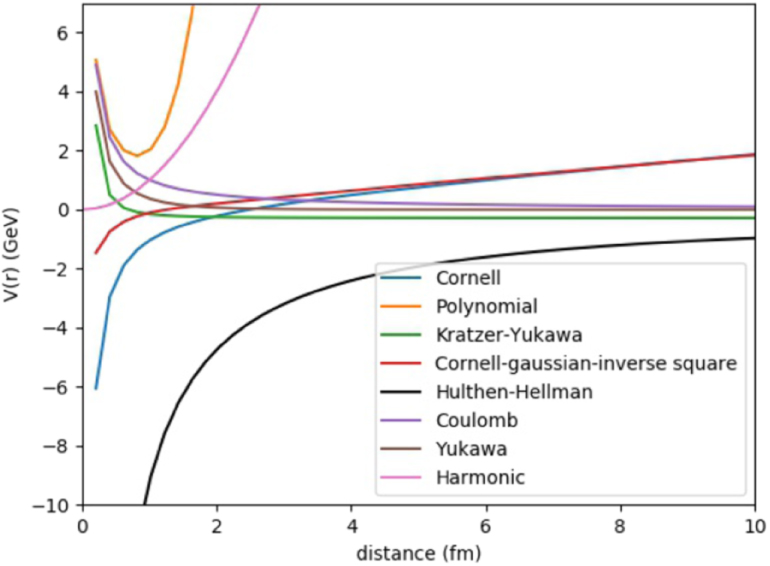
Table 2. Different potentials, it's mathematical form and the system studied.
| Potential | V(r) | System studied |
|---|---|---|
| Cornell |

|
 , ,  , ,  , , 
|
| Polynomial |

|

|
| Cornell, Gaussian and inverse square |

| B and D mesons |
| Kratzer and screened Coulomb |

|

|
| Yukawa, linear and harmonic |

|

|
From table 2 we can see that phenomenological potential study is quite successful in heavy quarkonium systems. For small quark separations (∼4fm) the nature of most of the potentials are similar (figure 1) therefore, the mass spectra estimated are also showing similar pattern. Therefore, we expect that the decay properties estimations should also be nearly the same. However, very limited work has been done so far for heavy tetra and pentaquarks.
We have compared the mass spectra of a few states of charmonium in table 3 and bottomonium in table 4 (without spin correction) in some potentials. For 1S, all potentials approach gave the same result (9.460 GeV for bottomonium and 3.096 GeV for charmonium, which is not shown in the table). Mass spectra do not show much deviation for 2S and 1P states.
Table 3. Mass spectra for charmonium states in different potentials (in GeV).
| V(r) | Constants | 2S | 1P | 1D |
|---|---|---|---|---|
 [124] [124] | a = 0.2 GeV2, b = 1.244 | 3.686 | 3.225 | 3.504 |
 [149] [149] | a = 0, d = 0, b = 0.202 GeV2, c = 1.664 | 3.689 | 3.262 | 3.515 |
 [155] [155] | a = −0.2860 GeV, b = 0.001 GeV, c = 0.1306 GeV, p = 0.0022 GeV | 3.686 | 3.295 | 3.583 |
 [151] [151] | a = 10.7 GeV, b = 6.39286 GeV, d = −0.495 eV, p = 7.1 GeV | ⋯ | ⋯ | 3.6861 |
 [165] [165] | a0 = −1.591 GeV, b = 9.649 GeV, c = 0.028 | 3.686 | 3.521 | 3.768 |
Table 4. Mass spectra for bottomonium states in different potentials (in GeV).
| V(r) | Constants | 2S | 1P | 1D |
|---|---|---|---|---|
 [124] [124] | a= 0.2 GeV2, b= 1.569 | 10.023 | 9.691 | 9.864 |
 [149] [149] | a = 0, d = 0 b = 0.202 GeV2, c= 1.664 | 10.023 | 9.608 | 9.814 |
 [155] [155] | a = −0.0723 GeV, b = 0.001 GeV, c = 0.050 GeV, p = 0.0022 GeV | 10.569 | 9.661 | 9.943 |
 [165] [165] | a0 = −1.591 GeV, b = 9.649 GeV, c = 0.028 | 10.023 | 9.861 | 10.143 |
Baryons are also extensively studied in different models. The GBE interaction and OGE describe interquark interactions successfully to get baryon spectra. Both the interactions gave light and heavy baryon (ground state) spectra. According to Mathur et al [197], the OGE model cannot accurately represent the Roper resonance, but the GBE model can. For light baryons, this is a significant distinction between the GBE and OGE models. Due to improved experimental facilities like BaBar, CLEO, Belle, CDF, and LHCb, as well as theoretical advancements, research in baryons with charm and bottom quarks have made outstanding progress in recent years. Most of the charmed and bottom baryon ground states have been explored experimentally. However, excited heavy baryon states are yet to be discovered.
Diquark correlation may be applied to the bag model, string model, and potential models in the case of baryons. It was anticipated that the diquark correlation for the qQQ baryon would be perfect. The diquark approach can be applied to different potential models also. Phenomenological potential models and QCD sum rules mainly discussed baryons with heavy quarks. Bag model were also able to discuss the light baryons, including the baryon octet and decuplet.
The Nambu–Jona–Lasinio (NJL) model was one of the successful approaches primarily inspired by the idea of representing baryon as a soliton. However, chiral symmetry is violated in the case of heavy quarks, and there is no Goldstone boson exchange. It should also be noted that the chiral constituent model does not have a confinement mechanism [198].
Lattice QCD has explained some of the XYZ tetraquark states and large momentum transfers. However, quantitative confirmation is still needed. The predictions provided by lattice QCD are reliable only for hadrons with heavy quarks.
Therefore, we see that significant work is done on hadron spectroscopy of tetra and pentaquark systems in the framework of different potentials and models. But most of the works are concentrated on mass calculations. Decay study of such systems is also very important and required. Still, a lot of work is expected in this area.
Acknowledgments
We are grateful to the Manipal Academy of Higher Education for the financial support under Dr. T M A Pai scholarship program.
Data availability statement
The data that support the findings of this study are available upon reasonable request from the authors.