
Abstract
We present the first application of a new approach, proposed in (2016 J. Phys. G: Nucl. Part. Phys. 43 04LT01) to derive coupling constants of the Skyrme energy density functional (EDF) from ab initio Hamiltonian. By perturbing the ab initio Hamiltonian with several functional generators defining the Skyrme EDF, we create a set of metadata that is then used to constrain the coupling constants of the functional. We use statistical analysis to obtain such an ab initio-equivalent Skyrme EDF. We find that the resulting functional describes properties of atomic nuclei and infinite nuclear matter quite poorly. This may point to the necessity of building up the ab initio-equivalent functionals from more sophisticated generators. However, we also indicate that the current precision of the ab initio calculations may be insufficient for deriving meaningful nuclear EDFs.
Export citation and abstract BibTeX RIS

Original content from this work may be used under the terms of the Creative Commons Attribution 4.0 licence. Any further distribution of this work must maintain attribution to the author(s) and the title of the work, journal citation and DOI.
1. Introduction
Different energy scales that appear in nuclear systems suggest a theoretical approach based on effective field theories (EFT), which use relevant degrees of freedom adapted to a given energy scale [1]. A remarkable example is the chiral effective field theory (χ-EFT) [2, 3]: by using neutrons, protons, and pions as degrees of freedom, χ-EFT is able to provide consistent description of numerous observables in atomic nuclei. Chiral interactions are used in the framework of ab initio methods to solve the many-body Schrödinger equations, employing controlled approximations. The numerical solutions require huge computational resources; for this reason, actual state-of-the-art ab initio calculations are limited to nuclei that are not too heavy and/or close to (semi)magic systems [4–7]. In particular, the description of open-shells nuclei has a recent history, started with the Gorkov–Green's function approach [8].
Another example of successful effective theory is the approach based on nuclear energy density functionals (EDFs) [9, 10]. Nuclear EDF is a versatile tool that, at low computational cost, allows us to describe properties of atomic nuclei across the entire nuclear chart from drip-line to drip-line and from light to super-heavy nuclei. The underlying non-relativistic functionals are usually obtained from phenomenological two-body potentials called functional generators, which have radial form factors of zero-range, for Skyrme [11, 12], or finite-range, for Gogny [13] implementations, with coupling constants adjusted to reproduce selected nuclear observables. In addition to finite nuclei, also infinite nuclear matter properties can be addressed within the EDFs formalism [14–16], and included among the observables.
In reference [17], it was shown that Skyrme EDFs have reached their best in terms of reproducing the experimental observables. As a consequence, several groups are exploring new forms of functional generators to improve precision of describing data [18–22]. The resulting functionals are then adjusted following standard procedures based on constraining the coupling constants to a given set of nuclear observables [23, 24].
In this article, we aim to explore a complementary approach, which is based on explicitly bridging the ab initio methods with the nuclear EDFs. Formal connections between the two approaches are the subject of recent studies [25, 26]. Furthermore, in reference [27] the density matrix expansion formalism has been used to obtain a set of functionals microscopically constrained from chiral effective field theory interactions. Here, we proceed by fitting parameters that enter the energy functional directly to metadata generated by the ab initio calculations, using the method suggested in reference [28]. In reference [28] this method was applied adjusting the Skyrme coupling constants to metadata generated by the Gogny functional. In this work, we perform a realistic application of the method by employing full-fledged ab initio calculations that use self-consistent Green's function (SCGF) [29] methodology with the chiral interaction NNLOsat [30].
The paper is organised as follows: section 2 briefly recalls the SCGF (section 2.1) and EDF (section 2.2) methods, and explains the formalism to derive the model functionals (section 2.3). Results are discussed in section 3 and conclusions are given in section 4.
2. Theoretical
2.1. Self-consistent Green's function method
We separate the nuclear many-body Hamiltonian Ĥ = Ĥ0 + Ĥ1 into a noninteracting part  , with the auxiliary one-body operator Û, and the interacting part defined as
  . We express the nuclear Hamiltonian in second quantisation as
where  are the single-particle energies of Ĥ0. By solving the corresponding Schrödinger equation,

one obtains the ground-state energy  and wave function
  of the nuclear system. The exact solution of equation (2) is very complicated and it is typically limited to systems with very few number of nucleons [31]. Rather than calculating the full many-body wave function, it is possible to expand the solution of the Schrödinger equation in terms of the propagation of single-particle excitations and the correlated density matrix of the system by using SCGF method [29]. These excitations represent basic collective degrees of freedom of the nucleus and they are described by the one-body Green's function, or propagator Gαβ. Using the Källén–Lehmann representation [32, 33], Gαβ takes the form
Here the complete set of eigenstates  ,
,  with eigenvalues
  ,
,  introduce the intermediate (A ± 1)-body systems. Then,
  and
and  are, respectively, the excitation energies of the propagating quasi-particle (index n) and quasi-hole (index k) states.
The propagator given in equation (3) satisfies the Dyson equation

where  is the propagator for the noninteracting system Ĥ0, and
  is the irreducible self-energy. The latter represents the nonlocal and energy-dependent potential to which each nucleon is subjected when interacting within the nuclear medium. The nonlinearity of equation (4) in terms of Gαβ(E) requires an iterative procedure to reach convergence. The full self-consistency is required to satisfy fundamental symmetries and conservation laws [34].
A crucial ingredient of equation (4) is the self-energy. This is composed of three parts as

which, respectively, are the auxiliary potential, static mean-field, and energy-dependent component. To perform calculations of the energy-dependent component, in this work we employ the algebraic diagrammatic construction method [35, 36] up to third order, denoted by ADC(3). We refer to reference [37] for a more pedagogical introduction of the method. The accuracy of ADC(3) can be estimated to be of the fourth order in Ĥ1, giving in practice an error of 1% of the total binding energy [37].
Another important aspect of the ab initio calculations is the presence of explicit three-body interaction  . By means of the modified Migdal–Galitski–Koltun sum rule [38], we can write the ground-state energy of the system as,

where  is the highest quasi-hole energy, namely
  . The determination of the expectation value of the three-body interaction would require calculation of many-body propagators. Instead, assuming that the magnitude of the three-body term is smaller than that of the two-body term, we take the lowest order approximation for the Hamiltonian, leading to

where ραβ is the one-body density matrix.
2.2. Model energy density functionals and generators
Having defined the main theoretical aspects of the ab initio method employed in this article, we now define the model energy density functional as

The different terms correspond to average values, evaluated with respect to a Hartree–Fock (HF) state, of the kinetic energy ![${T}^{1\text{B}}\left[\rho \right]\equiv \langle {\Phi}\vert {\hat{T}}^{1\text{B}}\vert {{\Phi}\rangle }_{\text{HF}}$](https://content.cld.iop.org/journals/0954-3899/47/8/085107/revision2/gab8d8eieqn17.gif) , Coulomb potential
, Coulomb potential ![${V}^{\text{Coul}}\left[\rho \right]\equiv \langle {\Phi}\vert {\hat{V}}^{\text{Coul}}\vert {{\Phi}\rangle }_{\text{HF}}$](https://content.cld.iop.org/journals/0954-3899/47/8/085107/revision2/gab8d8eieqn18.gif) , and interaction components
, and interaction components ![${V}_{j}^{\text{gen}}\left[\rho \right]\equiv \langle {\Phi}\vert {\hat{V}}_{j}^{\text{gen}}\vert {{\Phi}\rangle }_{\text{HF}}$](https://content.cld.iop.org/journals/0954-3899/47/8/085107/revision2/gab8d8eieqn19.gif) . The operators
. The operators  represent our choice of the generators to build the functional, whereas Cj are the coupling constants we need to adjust on (meta)-data.
In the present article, we define generators  , based on ten individual terms
  and
and  for i = 0, 1, 2, and
  ,
,  ,
,  , and
, and  of the Skyrme functional generator [12], that is,

where  is the antisymmetric operator for combinations of
  and
and  . We refer to reference [39] for more details.
To determine the coupling constants of the interaction using ab initio methods, it is convenient to transform the generators given in equation (9) to linear combinations that give specific isoscalar/isovector terms of the functional [28]9. This is done by means of the following matrix relation,
We explicitly included only the vector part  of the tensor term [40], which in the case of spherical symmetry considered here gives the only non-zero contribution. Note that the terms associated with the
  and
and  generators do not allow for the separation of isoscalar/isovector terms, and therefore we keep them identical to the corresponding terms of the Skyrme generator in equation (9). The generators listed on the left-hand side of equation (10) are then used as generators,
  , j = 1–10, that define the functional in equation (8).
2.3. Derivation of the functionals
In the electronic density functional theory [41], one uses the Levy–Lieb constrained variation [42–45] to obtain the ground state energy of the system. This procedure consists in a two-step minimisation,

where  stands for the Coulomb potential and symbol min|Ψ⟩→ρ denotes an inner (first-step) minimisation over all correlated many-body states |Ψ⟩ that have a common fixed one-body density profile ρ(r). The outer (second-step) minimisation is then performed over all possible profiles ρ(r), and, in such a way, the global minimum of energy, and thus the exact ground-state energy Eg.s. is obtained.
The inner minimisation can be conveniently performed by an unconstrained minimisation of the Routhian  at fixed one-body external potential U(r) that plays a role of the Lagrange multiplier,

This gives the energy E[U] = R[U] − ∫drU(r)ρ(r) and density ρ[U] as functionals of the potential U(r). Assuming that the inverse functional U[ρ] can be found, we obtain the exact energy density functional,

which after the outer (second-step) minimisation gives again the exact ground-state energy Eg.s..
In the case of a nuclear system, we consider the analogous first-step variation consisting in the minimisation of the Routhian  as
as

where Ĥab is the Hamiltonian of the system, equation (1). We use the superscript ab to indicate that it is the Hamiltonian of the ab initio theory, distinguishing it from the Hamiltonian used to build the model functional. The minimisation gives us many-body states as functionals of the external potential, |Ψ(U)⟩.
The integrand on the right-hand side of equation (14) introduces a perturbation of the ground-state |Ψg.s.⟩. The response of the system to the perturbation causes a change in the density ρ. If we were able to probe the system with all possible potentials U(r), we would have obtained the functional Eab[U] ≡ ⟨Ψ(U)|Ĥab|Ψ(U)⟩, and then, as above, the exact energy density functional Eab[ρ]. In the second step, the functional Eab[ρ] is minimised with respect to ρ, which gives the exact ground-state energy  and density ρg.s.(r).
Being unable to perturb the system with an infinite number of external potentials, let us introduce a discrete finite set of pre-defined external potentials ui(r) and their corresponding strengths λi, whereby the first-step minimisation (14) becomes,

With this restriction, the ab initio energy and density, Eab(λi) and ρab(λi), become functions (not functionals) of the finite set of strengths λi. Obviously, we now do not know what is the full energy density functional Eab[ρ] in the infinite-dimensional space of all possible one-body density profiles, however, we know it exactly on a finite-dimensional manifold of densities parametrised by strengths λi. Recall that this manifold still contains the point λi = 0 that corresponds to the exact ground state. The second-step variation would now correspond to the minimisation of function Eab(λi) in finite dimensions.
As proposed in reference [28], we now conjecture that a meaningful manifold of ab initio densities ρab(λi) can be obtained not by pre-defining external potentials ui(r), but by perturbing the system with generators that are going to be used for modelling the functional, section 2.2, that is,

Since the unrestricted minimisation of the Routhian is equivalent to finding its exact ground state |Ψab(λi)⟩ and eigenvalue Rab(λi), we have

Formally, by replacing minimisation (15) with minimisation (16), we do not make any new assumptions. Indeed, the previously made assumption about the reversibility of the functional ρ[U] suffices. It stipulates that for any density ρ(r) generated by the latter minimisation there exists a potential U(r) that would have generated it by the former minimisation. However, when using minimisation (16) we do not have to pre-define any potential or, for that matter, we do not have to know it at all.
Since our goal is to use the ab initio energies with perturbation λi as metadata to determine the coupling constants of our model functional, we impose that the ab initio energy can be expressed in the form of functional (8), that is,

Equation (18) constitutes the central point of our approach. At first glance, it looks like an impossible miracle: it expresses the exact ab initio energy as a functional of the exact ab initio one-body density profile ρ(r) only. However, this is, in fact, exactly the main statement of the rigorous DFT [41, 46, 47]. Without repeating here the related arguments, at this point it is nevertheless worth summarizing the three assumptions we did make when formulating equation (18):
- (a)We use a specific form of the density functional restricted to a few terms given by Skyrme generators (9). Obviously, the exact functional of equation (13) does not have to have such or a similar form. This is why in our approach we aim to derive a model functional and not the exact one. Nevertheless, a successful phenomenology of modelling nuclear phenomena by Skyrme-type functionals supports the idea of the model formulated in equation (18).
- (b)Skyrme functional depends not only on the local density profiles ρ(r) for neutrons and protons, but also on a few second-order quasilocal densities [40, 48]. Although it can be rigorously proved that any arbitrary local density profile can be modelled by a density profile of a Kohn–Sham Slater determinant [49], a simultaneous modelling of local and quasilocal densities is only an approximation.
- (c)When matching left- and right-hand sides of equation (18), we use a specific finite set of Lagrange multipliers λi. Had the form of functional on the right-hand side been exact, we could have used any set of λi. However, for the specific model functional we use, the results may depend on the specific values of the Lagrange multipliers. Our choice of using values around λi = 0 constitutes, therefore, another approximation.
In addition, considering that the Kohn–Sham kinetic energy represents a good approximation to the one-body kinetic energy, we assume that

If in the ab initio Hamiltonian the two-body center-of-mass correction  is included, it needs to be removed from the left-hand side of equation (18). Moreover, we suppose that the Coulomb contribution in the ab initio Hamiltonian is close to the Hartree–Fock average in the functional, namely,

Based on these two additional assumptions, we subtract the kinetic and the Coulomb energies from both sides of equation (18), rewriting it as
where  is the ab initio potential. The coupling constants Cj can now be obtained by linear regression analysis to best match the ab initio results appearing on both sides of equation (21) and determined for a meaningful set the strength parameters λi.
To evaluate the right-hand side of equation (21), we used standard expressions for Hartree–Fock expectation values of two- and three-body generators, that is,


where  is the ab initio one-body density matrix, and
  and
and  are the antisymmetrized two- and three-body matrix elements.
To evaluate the left-hand side of equation (17), we have to take into account the fact that the SCGF solver is not able to separate the different potential contributions to the Routhian in equation (16), but it provides us with the total interaction energy, defined as

This gives equation (21) in the form
that is, we have to evaluate the ab initio expectation values of the Coulomb potential and functional generators.
For a generic two-body operator, the exact expectation value ⟨Ô2B⟩ ≡ ⟨Ψ(λi)|Ô2B|Ψ(λi)⟩ is given as infinite expansion in terms of the effective interaction and dressed propagators, as sketched in figure 1 (first line). From a practical point of view, such a summation becomes computationally difficult, because the dressed propagators contain many poles that multiply matrix elements of every interaction line. Therefore, we approximate the single-particle propagator Gαβ(E) with an optimised reference state (OpRS) propagator [50, 51], defined as

This is a model propagator for independent-particle states with energy  OpRS and wave function ϕ. Such a propagator contains a reduced number of poles compared to the dressed one, while the energies and wave functions of the OpRS propagator are constrained to give the same momenta of the dressed propagators. We estimate ⟨Ô2B⟩ using the dressed propagators in the leading order (LO), or Hartree–Fock average, and the OpRS propagators in the next-to-leading order (NLO) and in the all-orders re-summation diagrams, as depicted in the second line of figure 1. We account for higher orders with the ph-, pp- and hh-RPA (random phase approximation) insertions, respectively, in the ring and ladder re-summation diagrams. At the cost of introducing a small error of the density, the use of the OpRS propagator allows us to remarkably speed up calculation of
  and
and  , which, otherwise, would not have been possible.
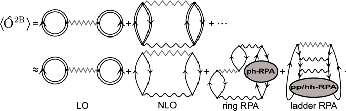
Figure 1. Diagrammatic representation of the expectation value of the two-body operator Ô2B, represented by zigzag lines. Double straight lines are used for dressed propagators, single lines for OpRS propagators, and wavy lines for two-body effective interactions. These are Feynman diagrams in the energy formulation, that is, they include forward and backward propagation. In the right-hand side of the first line, we can recognise the infinite expansion in term of dressed propagators. In the second line, we use the ph-RPA and pp/hh-RPA insertions to estimate contributions from NNLO and higher order terms.
Download figure:
Standard image High-resolution image3. Results
In this section, we present our results obtained using SCGF with ADC(3) approximation. We chose the interaction NNLOsat [30] for the two-body and three-body sector. We made this choice since this interaction has been optimised to reproduce ground state energies and radii for isotopes up to mass A = 24 and it has been shown to predict accurate saturation properties also for larger isotopes and for infinite nuclear matter [52–55].
The SCGF calculations were performed using a basis of spherical harmonic oscillator wave functions with oscillator energy ℏω = 20 MeV. The model space was limited to states with principal quantum numbers smaller or equal than Nmax. In terms of computational resources, even if the present technology allows calculations up to Nmax = 13, this would require a too large amount of CPU hours to complete the full set of perturbations required in the current analysis. We thus decided to limit the model space to Nmax = 9. This model space may converge poorly to the experimental values, but, in the first attempt at this approach, our attention focus on the validity of the method rather than on the accurate prediction of the experimental masses. Note that recent calculations in reference [55] showed that ℏω = 20 MeV is optimal for converging 16,24O but only nearly optimal for the heaviest isotopes we consider here. However, this small de-tuning has little effects when compared to our Nmax = 9 truncation. Therefore, we used the same oscillator frequency for all computations in this work.
In figure 2, we show binding energies per nucleon, E/A, for seven nuclei 16O, 24O, 34Si, 36S, 40Ca, 48Ca, and 56Ni. Each nucleus is in the configuration corresponding to fully filled spherical orbitals. These nuclei represent all available convergent ADC(3) calculations among the magic systems between 16O and 56Ni.
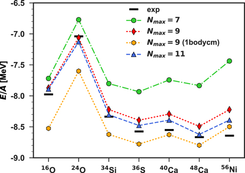
Figure 2. Binding energies per nucleon E/A for different nuclei. Theoretical values correspond to the unperturbed cases (λi = 0). Calculations were performed with NNLOsat [30] interaction, ℏω = 20 MeV, and model space specified by Nmax in the legend. Black rectangles represent the experimental values taken from reference [56].
Download figure:
Standard image High-resolution imageValues of E/A are reported for three choices of the size of model space: Nmax = 7, 9, and 11, to be compared with the experimental values taken from reference [56]. The convergence in terms of Nmax is not fully achieved; nevertheless, with increasing Nmax, most binding energies decrease towards the experimental values. The model space of Nmax = 7 appears to be too small to reproduce experimental results. For Nmax = 11, the maximum difference with experiment appears for 56Ni, with the difference of around 3% of the total energy. This discrepancy is a combination of the 1% error on the correlation energy that is associated with the ADC(3) truncation [37] and of the accuracy of state-of-the-art chiral nuclear forces [55, 57]. In absolute terms, the calculated binding energy of 56Ni is more than 10 MeV above the measured value. Such a deviation is much larger than the standard deviation of typical EDFs, which is of the order of 1 MeV [24, 58]. Clearly, with the model space truncation discussed below, the overall accuracy with respect to predicting the experiment is too poor to obtain novel functionals capable of reducing the discrepancies between the EDF approach and the experiment. However, our goal is to reproduce the ab initio energies, irrespective of their detailed agreement with experiment.
Typical ab initio computations subtract the kinetic energy of the centre of mass to directly access the intrinsic ground state energy [59]. This implies adding a one- and a two- body correction terms to the nuclear Hamiltonian [37, 60]. The result of retaining only the one-body term is shown in figure 2 for Nmax = 9 as '1bodycm' and it amounts to an overcorrection. However, this additional discrepancy will not affect our goal of investigating the consistency between microscopic results and the functionals that they generate. For our purposes, it is technically simpler to drop the two-body center-of-mass correction because it avoids further approximations in the way the kinetic energy is treated in the SCGF and EDF approaches. Since the EDF results also depend on the number of oscillator shells included in the model space [61], we fixed the model spaces of both approaches to be Nmax = 9 (1bodycm) for the following analysis.
In the model functional, equation (8), we consider generators of zero-range contact interaction (Skyrme-like) defined in equation (10), namely,  ,
,  ,
,  ,
,  ,
,  , and
, and  . Subscripts T = 0 and 1 denote generators inducing terms of the functional that depend on isoscalar and isovector densities, respectively. Such a link between generators and densities is valid only on the EDF level; for the chiral interactions used in our SCGF computations, already at the next-to-leading order in powers of the interaction, expectation values of generators contain contributions from both isoscalar and isovector densities.
We perturbed ground states of each of the seven selected nuclei using four different intensities of the perturbation strength λi, separately for each of the 10 generators. In this way, we obtained 284 converged results10, which represent our full database of the perturbed and unperturbed ground-state energies. The choice of using non-zero values of λi separately for each  represents a compromise between the volume of calculations and a coverage of the full manifold in the space of perturbations λi. Obviously, the larger the λi's the wider is the density space probed, however, if perturbations are too strong, the numerical SCGF solutions may diverge. In practice, for each generator, we have found a most suitable range of values of λi's that were used in the final calculations.
3.1. Estimated errors on the SCGF calculations
Figure 3 shows the ab initio energies in function of λi calculated for different perturbations  in 34Si. We had expected that the value at λ = 0 (black triangle) would be the one with the lowest energy Eab(0), because for any state different than the exact ground state |Ψ(0)⟩, the variational principle stipulates that

assuming, of course, that the ab initio energies are calculated exactly. From the plot, it is evident that there are cases of energies Eab(λi) smaller than Eab(0) in violation of the variational principle. For the perturbations induced by the three-body generator  (hexagons), the energy does not present a minimum, but increases monotonically with λi. This effect can be partially related to the way the contribution of the three-body interaction is extracted. In fact, we can estimate only the leading order as in equation (7).
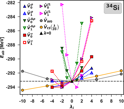
Figure 3. Perturbed ab initio energies compared with the unperturbed energy in 34Si. Symbols shown in the legend correspond to different generators  . The full triangle represents the unperturbed energy at λi = 0 and the dashed line shows the reference value of Eab(0).
Download figure:
Standard image High-resolution imageThe violation of the variational principle must be traced back to a series of approximations used to calculate the SCGF results. To make any sensible use of these metadata when fitting the functional coupling constants, we thus have to estimate the uncertainties associated with the SCGF calculations.
The major source of error in our calculation is probably related to the subtraction procedure of the perturbation energies from solutions given by the minimisation of the Routhian. For simplicity, we further assume that only one perturbing potential contributes to this uncertainty. The resulting subtraction error,  , associated with the value of Eab(λi) can be estimated as

where ⟨⟩RL, ⟨⟩NLO, indicates the truncation, respectively, up to ring and ladder RPA, to NLO approximation. Such error can be viewed as a relative error between the perturbed solutions and the unperturbed one. In figure 4, we show the subtraction errors  calculated for perturbations induced by the potential
  in 34Si. As expected, this error is zero for λi = 0 and grows rapidly with increasing values of the perturbation strength parameter λi.

Figure 4. Examples of errors associated with the ab initio energies Eab(λi), estimated in 34Si for perturbations related to generator  . The darker shadow represents the error
  given by equation (28). The lighter shadow represents the error
  extracted from the Hellmann–Feynman theorem, equation (31).
Download figure:
Standard image High-resolution imageWe also found another way to estimate uncertainties of the SCGF calculations, which is independent of the approximately calculated average values of the perturbation potentials  . Indeed, we can determine such estimates by using the well-known Hellmann–Feynman theorem [62]. For any Hamiltonian
  that depends explicitly on the parameter λ, the theorem states that

Equation (29) is valid under the condition that |Ψ(λ)⟩ is an eigenstate of Ĥλ, Ĥλ|Ψ(λ)⟩ = Eλ|Ψ(λ)⟩, or an Hartree–Fock wave function [63], or a variational wave function [64]. However, when the wave function is expanded in a truncated basis [65], or it is a solution of a perturbative expansion [64], the Hellman–Feynman theorem is violated. The ground-state wave function in the SCGF method is not variational because the ADC(3) approximation is a truncated expansion. The degree to which the Hellman–Feynman theorem is violated then illustrates the degree of violation of the variational principle.
The derivative at λ = 0 in the left-hand side of equation (29) can be, for small values of λ, determined by the finite difference method,

In our numerical test, we studied the case of the perturbation given by  , that is, by the full potential Vtot(0), equation (24), that defines Ĥab at λi = 0. This compares the finite difference of the energy calculated for the perturbed cases (λ and −λ) with the average value of the interaction energy in the unperturbed case (λ = 0). Such a comparison offers an estimate of the difference between the approximated energy in the ADC(3) method and the exact energy. Consequently, we define the error of the ab initio energy as

where subscript H–F stands for the error extracted from the Hellmann–Feynman theorem. This error represents an absolute error of the total energy that is due to the approximated solution of the SCGF method. It depends on the nucleus, but we assume it is independent of the perturbation, namely the value calculated at λ = 0 is attributed to all perturbed and unperturbed total energies of a given nucleus.
In the case of Nmax = 9 (1bodycm), the violation of the Hellmann–Feynman theorem, as defined in equation (31), is for lighter (heavier) nuclei studied in this paper equal to about 1% (3%–4%) of the total energy. This error is larger than the estimate provided in reference [37], because it gives a cumulative effect resulting from the ADC(3) truncation and reduced model space.
In figure 4, we also show the Hellmann–Feynman error  determined in 34Si. We see that for this particular generator,
  ,
,  is more than twice larger than
  . We checked that in most cases considered in this paper
  , even in very light nuclei. Given the very different magnitude and sources of the subtraction and Hellmann–Feynman errors, we decided to keep them separate and perform two independent analyses of the coupling constants.
In view of the identified uncertainties, we can now conclude that the explicit violation of the variational principle obtained for Eab(λi ≠ 0), see figure 3, can be considered acceptable consequences of the inherent imprecision encountered in the SCGF approach.
3.2. Linear regression analysis to determine the coupling constants
From the set of ab initio calculations described in section 2.3, we obtained d = 284 equations (25) whose left-hand sides represent regression dependent variable yi, i = 1–284, and whose p expectation values on the right-hand sides form the matrix of features, that is,

where each coupling constant Cj corresponds to a generator of the model functional given in equation (8).
Introducing for compactness the vector notation: C = (C1, ..., Cp) and y = (y1, ..., yd), we build the penalty function by of the least-square method as

where the weight matrix W is a diagonal matrix with elements Wii = wi. We define the weight of each data point as the inverse of the estimated error squared,

where Δyi is composed of three contributions [66],

 is the error attributed to the SCGF approach, namely, we take it as
  (28) or
  (31). Δynum is the numerical precision of the SCGF calculations, which is smaller that 5 × 10⁻⁵ MeV and can be neglected. Δymod represents the error associated with the model itself, which is entirely unknown, and thus it has to be tuned to normalise the penalty function χ2. Starting from an arbitrary value, Δymod can be increased iteratively up to the value at which the χ2 approaches the value of 1. Then, the penalty function in equation (33) satisfies the typical statistical normalisation condition χ2(C) → 1 at the minimum, and Δymod acquires interpretation of the Birge factor [67].
Minimisation of χ2 gives the solution Cmin, covariance matrix  , statistical error associated with the parameters, ΔCmin, and propagated errors of observables [66, 68, 69].
3.3. Fitted coupling constants
We minimise the χ2 defined in equation (33) using the two types of errors discussed in previous section. We thus obtain two sets of results: the one labelled DS(10), that is, obtained using the errors defined in equation (28) and that labelled DH–F(10)—using the errors defined in equation (31).
Given the large uncertainties of the metadata and the fact that they could be obtained only in fairly light nuclei with small isospin asymmetry, the resulting coupling constants are poorly determined with quite large error bars. This is particularly evident for the DH–F(10) set of parameters. The relative errors of the isovector coupling constants are often of the order of 100%, meaning that the obtained values are compatible with 0. The very large errors mean that the χ2 surface is fairly flat in these particular directions of the parameter space. As a consequence, when used to calculate atomic nuclei, the obtained coupling constants often immediately lead to finite-size instabilities [70].
The quality of the fit can be easily judged by inspecting relative residuals of equation (25), defined as

and for 56Ni shown in figure 5(a) for DS(10) and (b) for DH-F(10). For a good-quality fit, we would expect the residuals lie close to the dashed horizontal line, which indicates zero values. Rapid departures of residuals from zero, especially for the second-order isovector coupling constants, illustrate the fact that a reasonable description of the ab initio results in terms of Skyrme functional generators could not be obtained.
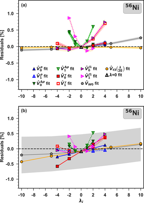
Figure 5. Residuals calculated for 56Ni with the parametrizations DS(10) (a) and DH–F(10) (b). Shadows show the corresponding propagated errors. For clarity, in (b) we only show the one corresponding to generator  .
.
Download figure:
Standard image High-resolution imageFor all nuclei and generators studied here, the residuals corresponding to the unperturbed systems (λ = 0) are around zero, whereas when λi moves away from zero, the residuals increase. In addition, they are not normally distributed, but they exhibit clear trends, meaning that the hypothesis formulated in equation (25) is not correct. Shadows shown in figure 5(a) represent the propagated errors of the corresponding observables obtained in the fit DS(10). For DH–F(10), the propagated errors are much larger, so in figure 5(b), for clarity we only show the one corresponding to generator  . We note that the propagated errors related to the violation of the Hellmann Feynman theorem are much larger than those corresponding to the subtraction errors, and thus they make it very hard to draw reasonable conclusions about the structure of the residuals.
We tested the performance of the obtained coupling constants in the description of infinite nuclear matter. For DS(10), we obtain a fairly reasonable energy per particle of E/A = −14.6 ± 0.2 MeV and saturation density of ρ0 = 0.132 ± 0.002 fm−3. The DH–F(10) provides slightly different values for the binding energy E/A = −16.0 ± 1.2 MeV and saturation density ρ0 = 0.128 ± 0.01 fm−3, but with much larger error bars than in DS(10). For both sets, the nuclear incompressibility K is also in the range of acceptable values [71]; in particular, we have K = 380 ± 17 MeV for DS(10) and K = 393 ± 143 MeV for DH–F(10). Other properties of infinite matter, such as the symmetry energy and its first derivative, are poorly determined, probably because the set of nuclei used for the fit is not rich enough to describe isovector properties of the nuclear medium sufficiently well. In particular, we find that the symmetry energy has a value compatible with zero within the error bars.
Another major drawback of the derived coupling constants is an unrealistic value of the effective mass. Although the effective mass is not strictly speaking an observable, we can extract information about its value from other many-body methods [72]. For the isoscalar effective mass, an acceptable range of values is m*/m ∈ [0.7–0.9], although it is worth mentioning that also other values are found in the literature. Both sets of coupling constants, DS(10) and DH–F(10), give effective masses that are off by roughly an order of magnitude (cf figure 7), and this is probably the main reason why they do not lead to realistic results when used in calculations of finite nuclei.
3.4. Constraints on the nuclear matter properties
Since a simple least-square minimisation does not provide us with satisfactory values of the effective mass, we also performed a constrained linear regression to drag the coupling constants towards reasonable values of m*/m. In this way, we want to test if the poor determination of the coupling constants, reflected in their large errors, can be exploited to improve values of the effective mass. Linear regression with constraints is a procedure in the spirit of the Bayesian inference, where a prior information about the parameters is known. Here we consider it in the form of the Tikhonov regularisation [73] or ridge regression [74], which consists of minimising the penalty function of the form
The Tikhonov parameter λT is a real positive number and b = Q[C] represents a system of f linear equations in parameters C with constant terms b. The final values of C will depend on λT. As one can see, equation (37) is defined as a sum of two terms:  , which depends on weights W, and
  , which depends on λT. Increasing the value of the Tikhonov parameter gives more importance to
  and eventually may deteriorate the description of data represented by
  .
.
We used one constraint, namely the definition of the in-medium isoscalar effective mass,

It is important to note that  depends explicitly only on one coupling constant,
  , however, implicitly, through the saturation density ρsat it non-linearly depends on all other coupling constants. We set the target value of the effective mass to b1 ≡ m*/m = 0.70 and in the Tikhonov term we varied the value of log10λT from −4 to 2. As an example, in
  we took the inputs used for DH–F(10). By implementing the Tikhonov regularisation, we aim to distinguish between two possible scenarios, namely, whether at an expense of a small deterioration of
  , description of effective mass can or cannot be improved.
In figure 6(a), we show the obtained evolution of the constrained parameters C in function of the Tikhonov parameter. As one can see, changes in the parameters happen around log10λT ≈ −2. Beyond this region, their values are quite stable.  ,
,  ,
,  and Ct3 are the coupling constants to which the constraint makes the largest impact. We already noted that these coupling constants were poorly determined by the unconstrained regression. In figure 6(b), we show relative contributions to the penalty function coming from the data points,
  , and from the constraint,
  , (see equation (37)). We see that the contribution of the constraint increases with λT up to log10λT ≈ −1.8 and after that it quickly drops to zero. At the peak of
  , the coupling constants begin to adjust to the requested value of m*/m. A further increase of λT decreases
  , because b1 − Q1[C] → 0, whereas the reproduction of the data points deteriorates and the differences
  increase.
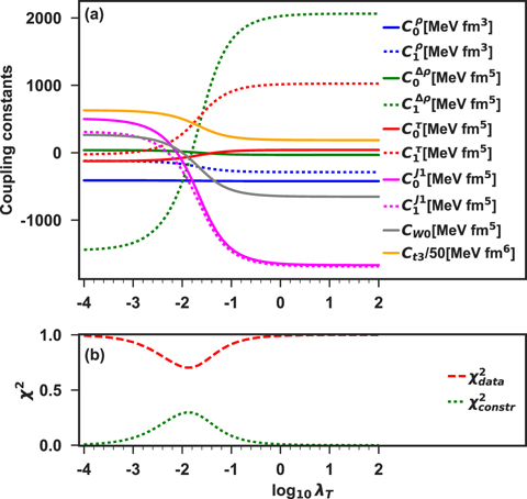
Figure 6. (a) Results obtained for the DH–F(10) coupling constants with m*/m constrained to 0.70 using the Tikhonov regularisation. (b) Contributions of the data,  , and constraint,
  , to the total penalty function
  (37).
(37).
Download figure:
Standard image High-resolution imageIn figure 7, we present nuclear matter properties ρsat, E/A, m*/m, and symmetry energy J obtained by the Tikhonov regularisation of the DH–F(10) coupling constants with m*/m constrained to 0.70. For small λT, the obtained values are equal to those corresponding to the original DH–F(10) results. In the region of log10λT between −2 and 0, nuclear-matter properties change abruptly, and effective mass is dragged towards the target value already at log10λT ≃ −1. In the region of log10λT ⩽ 0, nuclear-matter properties ρsat, E/A, and J cross their empirical values of ρsat = 0.17 ± 0.03 fm−3, E/A = −16 ± 1 MeV, and J = 32.5 ± 2.5 MeV (shown in grey) [71]. Such a crossing occurs at slightly different values of λT for the three quantities and before the effective mass reaches its empirical range. We note here, that for the NNLOsat chiral interaction, the corresponding nuclear-matter values read ρsat = 0.166 fm−3 and E/A = −14.5 MeV [30]. Beyond log10λT ≃ 0, nuclear-matter properties settle at values far away from the standard nuclear-matter values. When the effective mass approaches the target value of 0.70, the energy per particle E/A becomes too low and the symmetry energy becomes very large. We conclude that there is no region of the Tikhonov parameter where all four nuclear-matter quantities would be in their expected domains, even when the propagated errors (represented by shaded areas) are taken into account. In other words, the obtained incorrect values of the effective mass cannot be corrected by a small deterioration of the penalty function  .
.

Figure 7. Infinite nuclear matter properties: ρsat (a), E/A (b), m*/m (c), and symmetry energy J (d). Obtained by the Tikhonov regularisation of the DH–F(10) coupling constants with m*/m constrained to 0.70. Shadows show the propagated error bars and grey regions indicate the ranges of empirical values.
Download figure:
Standard image High-resolution image
4. Conclusions
Applying the methodology suggested in reference [28], we studied the link between the nuclear Skyrme functional and the NNLOsat chiral interaction used within the ab initio self-consistent Green's function calculations in ADC(3) approximation. We performed the ab initio calculations in seven light closed shell nuclei by perturbing their ground states with ten functional generators that define Skyrme functional. By employing the linear regression method, the obtained metadata were used to derive the functional coupling constants. We analysed two possible sources of uncertainties of the ab initio calculations: the first one related to approximate determination of average values of two-body potentials and the second one to an imprecise determination of nuclear ground states, for which we employed the Hellmann–Feynman theorem.
The obtained values of Skyrme coupling constants were very different than those typically obtained in phenomenological adjustments to nuclear observables. We have identified several possible reasons of such a result: first, it appears that a relatively high level of uncertainties arising in the ab initio calculations induces large uncertainties of the derived coupling constants, which then propagate to large uncertainties of the nuclear matter properties and to instabilities when solving the self-consistent equations. Second, it appears that the ab initio energies are poorly reproduced by the terms in the functional generated by the Skyrme zero-range potentials. Third, it appears that the information contents within the perturbed ground-state energies of light semi-magic nuclei is insufficient to properly determine Skyrme coupling constants, especially those corresponding to second-order terms depending on isovector densities.
Certainly, future research may be focussed on applications of ab initio technologies with improved overall precision, which would better correspond to the ambition of reducing discrepancies between the phenomenological EDF results and experiment. Another promising avenue would be to repeat present analyses by using finite-range functional generators. However, the most challenging aspect of the methodology proposed in reference [28] is the fact that it is based, similarly as most other generic ab initio DFT approaches, on the Levy–Lieb construction that essentially pertains to variational studies of ground-state energies. This is in opposition to the methodology of adjusting functionals directly to experimental data, where one uses not only ground-state energies, but also other essential observables like radii, deformations, or transition probabilities.
Acknowledgment
STFC Grants No. ST/M006433/1 and No. ST/P003885/1, by the Surrey's STFC Grants No. ST/P005314/1 and No. ST/L005816/1, and by the Polish National Science Centre under Contract No. 2018/31/B/ST2/02220. Numerical calculations were performed using computational resources provided by the CSC-IT Centre for Science, Finland, and using the DiRAC Data Analytic system at the University of Cambridge, operated by the University of Cambridge High Performance Computing Service on behalf of the STFC DiRAC HPC Facility (www.dirac.ac.uk). This equipment was funded by BIS National E-infrastructure capital Grant (ST/K001590/1), STFC capital Grants ST/H008861/1 and ST/H00887X/1, and STFC DiRAC Operations Grant ST/K00333X/1. DiRAC is part of the National e-Infrastructure.
Footnotes
- 9
In this paper, we use terms isoscalar and isovector, which are used in the nuclear density functional theory to describe parts of the functional that depend on the isoscalar or isovector densities, respectively. These terms are confusingly identical to terms isoscalar, isovector, or isotensor, which pertain to the covariance of the total interaction or functional with respect to rotations in the isospace. Both standards are now widely used in the literature, so it is probably too late to propose less a confusing terminology.
- 10
For 36S, 3 data points did not converge.