
Abstract
This paper presents a micro electromagnetic vibration energy harvester (VEH) that uses complementary metal-oxide-semiconductorcompatible 3D micro-electromechanical system coils and a ferromagnetic core to improve efficiency and output power. A systematic model is proposed to describe the nonlinear electromagnetic damping coefficient and nonlinear attraction between the magnet and the ferromagnetic core. The nonlinear model agrees well with the finite element calculation results. Then, a vibration model is established by considering nonlinear stiffness and damping coefficient to obtain the dynamic characteristics and output performance of the system. Furthermore, a numerical method is conducted to systematically investigate the influence of air gap and initial magnet offset under different excitation amplitudes. The simulation results indicate that with a smaller air gap, the output power is higher. Moreover, there is an optimal initial magnet offset in relation to the air gap to maximise the output power of the system. These conclusions and analysis models can be generalised and can be used as a guidance for the designs of similar structural devices. The results also show that the structure proposed in this study can significantly enhance the energy harvesting performance compared with published data of conventional VEHs.
Export citation and abstract BibTeX RIS

Original content from this work may be used under the terms of the Creative Commons Attribution 4.0 license. Any further distribution of this work must maintain attribution to the author(s) and the title of the work, journal citation and DOI.
1. Introduction
Sustainable energy supply technologies for wireless sensor networks (WSNs) have attracted the attention of numerous researchers in recent years. Harvesting energy from vibrations, which are abundant in the environment, is a promising technology that can replace batteries and has received considerable research interest. Current micro vibration energy harvesters (VEHs) are based on electromagnetic, piezoelectric, electrostatic, and triboelectric mechanisms, among which electromagnetic VEHs (EM-VEHs) have been the primary focus of research.
Recently, a large number of studies have been conducted to improve the output power and widen the frequency bandwidth; these studies have proposed strategies such as resonance frequency tuning [1], multi-stable dynamics [2, 3], two-degree-of-freedom (2-DOF) structures [4, 5], and hybrid-mechanism generators [6]. In these strategies, coils are fabricated as mechanical winding coils and micro-electromechanical system (MEMS) coils. Although mechanical winding coils can produce large output power, they may lead to an increase in volume and a reduction in integrity, making them unsuitable for WSNs. With the support of MEMS technology, coils can become complementary metal-oxide-semiconductor (CMOS)-compatible. However, most studies on micro VEHs have employed planar coils fabricated by MEMS technologies that result in large magnetic leakages, which limits the output performance the micro VEH. Recently, studies have also focused on the fabrication of three-dimensional (3D) micro-coils. Li et al developed an electroplating technology for high-density, small-diameter, high-aspect-ratio through-silicon vias, which can potentially be used to manufacture 3D micro-coils [7]. On this basis, Xu et al demonstrated a solenoid coil embedded in a silicon substrate via deep Si etching and Cu electroplating [8], and this coil can be integrated with the iron core to constrain the magnetic field, which has great potential to improve the performance of electromagnetic power MEMS devices.
This paper proposes a micro EM-VEH using CMOS-compatible 3D MEMS coils, which also applies a silicon steel sheet to constrain the magnetic field. This consequently reduces the leakage of magnetic flux and enhances its varying gradient, thereby achieving a significant enhancement of the output power and efficiency. Moreover, the overall structure is highly compact, which is suitable for integration with MEMS devices.
In this novel design, the application of the silicon steel sheet causes attraction on the magnet, and this consequently affects the stiffness curve of this system. The silicon steel can also influence the magnetic field distribution through the coils, which is related to the damping coefficient. However, none of the previously published models are suitable for the structure proposed in this study. Therefore, the nonlinear damping coefficient and the nonlinear magnetic force between the silicon steel and magnet need to be accurately modeled to predict the dynamic response and energy harvesting performance. Some studies calculate the magnetic force between permanent magnets based on magnetising current theory or magnetic dipoles method [9–11], which are unsuitable for the calculation of attraction of soft magnetic material and large dimension of silicon steel. Other studies used polynomial to simplify the nonlinear stiffness and damping coefficient [2, 12, 13], which inevitably caused force divergence at large displacements. For complicated nonlinear damping and stiffness, an extremely high order of terms must be employed. In this study, the expressions of arctangent and rational functions are proposed based on the classical magnetic dipoles theory and finite element method (FEM) to describe the complex nonlinear damping coefficient and stiffness respectively. Good agreement with FEM results was shown over a wide range of design parameters.
This paper is organised as follows. Section 2 provides the structural design and theoretical modeling of the vibration diagram. Then the nonlinear damping coefficient and magnetic force are modeled based on the theory analysis and FEM simulation. In section 3, the vibration response and output performance are numerically predicted based on the nonlinear model, and the influences of key design parameters and excitation conditions are performed and discussed. Finally, key findings and conclusions are presented and summarised in section 4.
2. Design and mathematical model
2.1. Theoretical model
Based on the structure and fabrication characteristics of 3D coils published in [8], an innovative MEMS VEH is designed (figure 1(a)). This device includes a permanent magnet, four pairs of planar springs, a pair of 3D coils, and a silicon steel sheet. The overall dimension of the device is 20 mm × 20 mm × 1 mm, which is made by bonding two silicon wafers. The springs are processed by wire cutting and are glued on both sides of the bonded substrate. The permanent magnet is placed on the center plane. By installing a shim at the bottom of the permanent magnet, the initial position of magnet can be offset from the center of silicon steel sheet, which is shown as x0 in figure 1(b).

Figure 1. (a) Overall structure of the micro VEH. (b) Schematic of magnetic path. (c), (d) Schematics of vibrations for the micro VEH.
Download figure:
Standard image High-resolution image3D MEMS coils are first applied in EM-VEHs, and a silicon steel sheet is integrated in this structure to constrain the magnetic field. The magnetising direction of the permanent magnet is parallel to the coils axis direction and perpendicular to the vibration direction. Compared with the traditional MEMS VEHs using planer coils, our model has a much higher magnetic flux gradient.
Figure 1(b) shows the symbols and geometrical parameters of the magnetic path. The air gap δ and initial magnet offset (IMO) x0 can significantly affect the dynamic response and output performance. Therefore, the influences of these two parameters are analyzed and optimised in this study.
The proposed EM-VEH is a typical 'spring-mass-damper' vibration system. Figures 1(c) and (d) show the vibration diagrams, where m is the mass of the vibration block. The stiffness terms include the mechanical stiffness Km (the resilience of the springs) and the electromagnetic stiffness Ke (the attraction between the magnet and the silicon steel sheet). When the eddy current loss in the silicon steel core is ignored, the electromagnetic damping de is related to the interaction between the magnet and coils, which leads to the conversion of vibration energy to electricity. dm is the mechanical damping which mainly includes the air damping effect. Considering that the air damping is significantly small compared with the electromagnetic damping, and that the proposed device can apply vacuum packaging technology to further reduce the energy dissipation, the mechanical damping dm is set to be zero in this study.
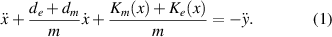
The equation of motion for the system is established by summing the dynamic forces on the block and this is described as follows:
The following sections describe the methods for modeling the stiffness and damping coefficient to predict the dynamic response and output performance accurately.
2.2. Electromagnetic damping
According to Faraday's law of electromagnetic induction, the electromotive force V can be derived as shown in equation (2):
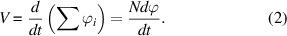
Here, ϕi is the magnetic flux through the ith loop, N is the total number of coil turns, and ϕ is the average magnetic flux along the axis of silicon steel. As the silicon steel can constraint the magnetic field and reduce the magnetic leakage, the magnetic flux along the coil axis can be assumed constant. Then the power consumed by the coils and the load circuit can be calculated using equation (3).
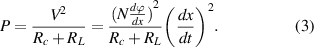
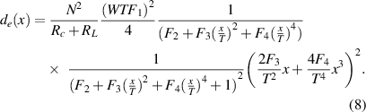
Here, Rc is the resistance of coil windings, which can be calculated using the classical direct-current resistance formula, and RL is the load resistance. Simultaneously, the power extracted by coils can also be expressed by the product of damping force and speed, as shown in equation (4), which is equal to the power consumed by the circuit.
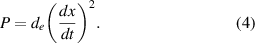
Hence the electromagnetic damping coefficient can be derived based on the conversion of energy, as shown in equation (5). Table 1 lists the coil parameters and impedance data.
Table 1. Coil parameters.
| Parameters | Value |
|---|---|
| Number of turns | 50 |
| Height of coils | 1 mm |
| Width of coils | 4.6 mm |
| Wire diameter | 100 μm |
| Turn pitch | 100 μm |
| Coil resistance | 0.9968 Ω ≈ 1 Ω |
The magnetic flux through one cross section can be calculated by:
Here, Bave is the average magnetic flux density normal to the section, and WT is the area of cross section. The magnetic field is generated by the magnet and the magnetised silicon steel. Hence, the magnetic flux density is a complicated nonlinear function of magnet size, silicon steel dimension, air gap, and magnet position. It is significantly difficult to derive a precise theoretical model to calculate the magnetic field distribution. Engel-Herbert et al presented an analytic expression for magnetic field of a single cubic permanent magnet in three dimensions [14]. The magnetic field strength along the magnetisation direction can be expressed by summing several arctangent terms of position coordinates. The magnetic field distribution of these two cases have the following common characteristics: (1) the magnetic induction intensity is symmetrically distributed, implying that the function is an even function: B(x) = B(−x) and dB/dx = 0 at x = 0 ; and (2) at infinity location the magnetic induction intensity decays to zero: B(±∞) = 0 . Inspired by this expression, in this study, the magnetic flux density is described by the arctangent and polynomial functions, as shown in equation (7).
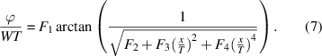
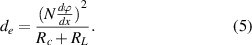
The ϕ/WT is the average magnetic flux density, which remains unchanged when the overall structure is scaled up or down, such that this function can be generalized to any similar geometrical structure. The coefficients Fi are related to the geometrical parameters, including the size of the air gap, magnet, and silicon steel sheet, and are also related to the coercive force of magnet. Equation (7) gives a functional form of the magnetic flux distribution, and the specific coefficient values need to be obtained by experiments or numerical simulations. In this study, magnetic flux data considering different positions and air gap sizes are simulated using MAXWELL 3D (figure 2(a)). The coercivity of magnet is 838 000 A m−1, and the relative permeability is 1.045. The B-H curve data of silicon steel sheet is listed in table 2. Table 3 presents the coefficients values of different air gaps, which show good agreement with the simulation results and also proved the practicality and validity of equation (7).
Figure 2. (a) Variation in magnetic flux with magnet displacement for different air gaps (0.3–1.5 mm). (b) Nonlinear stiffness curve of the planar spring. (c) Variation in attraction between magnet and silicon steel core with magnet displacement for different air gaps (0.3–1.5 mm).
Download figure:
Standard image High-resolution imageTable 2. B–H curve of DW465-50.
| H (A/m) | B (T) | H (A/m) | B (T) | H (A/m) | B (T) |
|---|---|---|---|---|---|
| 0 | 0 | 74.84 | 0.55 | 143.31 | 1.1 |
| 31.85 | 0.11 | 76.83 | 0.6 | 167.2 | 1.15 |
| 39.01 | 0.15 | 78.82 | 0.65 | 189.49 | 1.2 |
| 45.38 | 0.2 | 79.62 | 0.7 | 222.93 | 1.25 |
| 50.16 | 0.25 | 83.6 | 0.75 | 262.74 | 1.3 |
| 55.73 | 0.3 | 87.58 | 0.8 | 318.74 | 1.35 |
| 59.71 | 0.35 | 96.34 | 0.85 | 429.94 | 1.4 |
| 64.49 | 0.4 | 104.3 | 0.9 | 668.79 | 1.45 |
| 68.47 | 0.45 | 112.26 | 0.95 | 995.22 | 1.5 |
| 72.45 | 0.5 | 121.02 | 1 | 1592.3 | 1.55 |
Table 3. Fitting coefficients and correlation coefficient of equation (7).
| δ (mm) | δ/T | F1(×10−4) | F2(×105) | F3(×104) | F4(×104) | R2 |
|---|---|---|---|---|---|---|
| 0.3 | 0.6 | 3.357 | 0.854 | 3.869 | 1.013 | 0.99974 |
| 0.4 | 0.8 | 3.087 | 0.978 | 4.083 | 1.010 | 0.99968 |
| 0.5 | 1 | 2.828 | 1.133 | 4.634 | 0.925 | 0.99970 |
| 0.6 | 1.2 | 2.564 | 1.331 | 5.376 | 0.852 | 0.99947 |
| 0.7 | 1.4 | 2.266 | 1.573 | 5.732 | 0.866 | 0.99759 |
| 0.8 | 1.6 | 1.913 | 2.216 | 7.554 | 0.612 | 0.99364 |
| 0.9 | 1.8 | 1.407 | 2.962 | 11.426 | 3.319 | 0.99907 |
| 1 | 2 | 1.260 | 3.446 | 13.584 | 4.031 | 0.99913 |
| 1.2 | 2.4 | 1.083 | 4.165 | 17.152 | 6.007 | 0.99898 |
| 1.5 | 3 | 0.947 | 4.769 | 16.667 | 11.570 | 0.99734 |
Combining equations (5) and (7), the damping coefficient can be derived as follows.
2.3. Mechanical stiffness
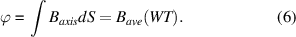
Owing to large deformation, the planar spring exhibits nonlinear stiffness characteristics along the thickness direction that can be approximated as a cubic polynomial. The spring parameters of this study are shown in figure 3, and the thickness is 60 μm. Every VEH has two planar springs arranged on the top and bottom sides of the silicon substrate.

Figure 3. Spring geometric parameters.
Download figure:
Standard image High-resolution imageThe nonlinear resilience of single planar copper spring is simulated using ANSYS, and is obtained by equation (9).
2.4. Electromagnetic stiffness
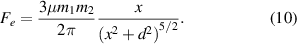
The magnet is attracted by the magnetised silicon steel core as shown in figure 1(c). In [11], the interaction force between two permanent magnets are derived by equating magnets to magnetic dipoles, as shown in equation (10), which is a rational function of position x.
However, in this study, the size of the silicon steel core is too large to be assumed as magnetic dipoles. Additionally, the magnetization intensity in the silicon steel core varies with the magnet position. Therefore, the function form of equation (10) needs to be adjusted to fit the structure of this paper. Based on this, an empirical rational function, as in equation (11), is proposed to describe the magnetic force between the magnet and silicon steel core.
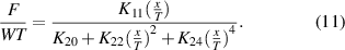
Here, F/WT is the attraction per unit facing area of magnet and silicon steel, which remains constant when the overall structure is scaled up or down. The coefficients Kij can be calculated for different geometrical designs.
Similar to equation (7), the discrete values of attraction with different positions and air gaps are simulated (figure 2(c)). The fitting coefficients are then derived from these values (table 4). The fitting results agree well with the simulation data.
Table 4. Fitting coefficients and correlation coefficient of equation (11).
| δ | δ/T | K11 | K20 | K22 | K24 | R2 |
|---|---|---|---|---|---|---|
| 0.3 | 0.6 | 1 | 0.003821 | 0.000885 | 0.000758 | 0.99954 |
| 0.4 | 0.8 | 1 | 0.005378 | 0.001470 | 0.000754 | 0.99969 |
| 0.5 | 1 | 1 | 0.007470 | 0.002138 | 0.000748 | 0.99977 |
| 0.6 | 1.2 | 1 | 0.010291 | 0.002792 | 0.000755 | 0.99975 |
| 0.7 | 1.4 | 1 | 0.013908 | 0.003584 | 0.000759 | 0.99964 |
| 0.8 | 1.6 | 1 | 0.018444 | 0.004343 | 0.000779 | 0.99984 |
| 0.9 | 1.8 | 1 | 0.024211 | 0.005294 | 0.000785 | 0.99979 |
| 1 | 2 | 1 | 0.031085 | 0.006417 | 0.000803 | 0.99984 |
| 1.2 | 2.4 | 1 | 0.050196 | 0.008623 | 0.000809 | 0.99985 |
| 1.5 | 3 | 1 | 0.090031 | 0.014400 | 0.000765 | 0.99897 |
2.5. Stiffness characteristics and potential curves
The total stiffness is the sum of the electromagnetic and mechanical stiffness. The IMO x0 can be controlled by installing an adjust shim on the bottom of the permanent magnet. It is worth noting that, due to the attraction of silicon steel core, an original deformation of planar spring is unavoidable when IMO is not zero, and this is shown in figure 4. The original deformation H0 is the real solution of equation (12).


Figure 4. The illustration of original spring deformation produced by magnetic force.
Download figure:
Standard image High-resolution imageThe relative position of the magnet, silicon steel core and planar spring at position coordinate x is shown in figure 5. For ease of reading, only one planar spring is plotted in figure 5. Then the restoring force produced by silicon steel core and planar spring at any position can be calculated using equation (13). The potential curve is derived by the integral of restoring force, and the equilibrium position is set to be the zero potential energy point.
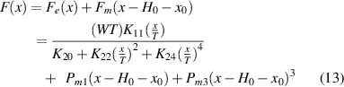
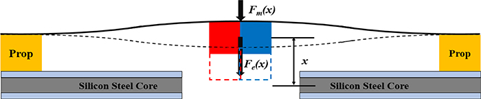
Figure 5. The illustration of relative position of magnet, silicon steel core and planar spring.
Download figure:
Standard image High-resolution image
The air gap can influence the magnetic force, whereas the IMO can affect the mechanical stiffness. Therefore, the influences of the air gap and IMO on the stiffness characteristics are analysed in this section. Figures 6(a) and (b) show the stiffness and potential energy curves for different air gaps when the IMO is 0 μm. With the decrease in the air gap, the stiffness of the system is improved, and because of this a steep potential energy curve is generated. Figures 6(c) and (d) delineate the stiffness and potential energy for different offsets when the air gap is 0.7 mm. The curves for other air gaps are similar. For a nonzero IMO, the curves demonstrate asymmetrical characteristics. The stiffness is considerably flatter on the right side of the initial position than on the left side, which indicates a lower potential energy on the right side. An increase in the IMO leads to a rapid increase and decrease in the stiffness on the left and right sides, respectively.

Figure 6. Stiffness curves and potential energy curves: (a), (b) curves for different air gaps with constant initial magnet offset (0 μm); (c), (d) curves for different IMOs with constant air gap (0.7 μm).
Download figure:
Standard image High-resolution image3. Numerical simulation and parameter analysis
3.1. Numerical method
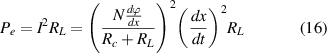
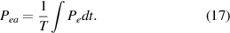
Based on the proposed model, the vibration dynamic of this system can be expressed using equation (15). The output power and other related performance parameters can be derived using equation (16). The average output power during steady-state operation is calculated by equation (17).
It is difficult to obtain the analytical solution of equation (15). Hence, in this section, the vibration equation is solved numerically. The excitation ÿ is given as a fixed frequency sine function, a0sin(ωt). The equation is discretised using the Runge–Kutta method. Then, the steady vibration response for a given initial state at a certain excitation condition can be numerically solved. In this study, the initial velocity is set to be zero, and the initial position is the lowest point of the potential energy curve, which is also the IMO. By adjusting the frequency and extracting the vibration amplitude and output power during steady-state at each frequency, the amplitude–frequency curves of system vibration and output performance can be obtained. The frequency corresponding to the maximum amplitude is the resonance frequency. The amplitude– frequency characteristics are related to the air gaps, IMO, excitation intensity and load resistance. Hence, for each design parameter or operating condition, it is necessary to calculate the amplitude– frequency curve separately, and then compare its performance.
3.2. Verification of numerical results
Equation (15) is a nonlinear second-order ordinary differential equation, which is very complicated. Hence it is difficult to derive the complete analytical solution. However, when the excitation acceleration is small enough, the vibration block only vibrates in a limited range, and then the system can be regarded as equivalent to a linear system which can be solved analytically. Therefore, in this study, the numerical method is verified by comparing it with the analytical solution under small excitation.
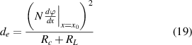
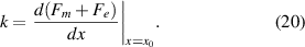
Equation (18) is the quasi-linear equation of equation (15). The constant electromagnetic damping coefficient de can be calculated using the gradient of magnetic flux at the bottom of potential well. The equivalent stiffness k is the first-order component of stiffness curve at the potential well bottom. The damping coefficient and stiffness can be calculated using equations (19) and (20).

The displacement amplitude during the steady state can be derived from equation (18), as:
Here, ωn
is the resonant frequency, which is  . The average electrical energy extracted by coils is,
Then, the power consumed by the load can be expressed as:
In this study, the output performances under 0.1 mg (1 g = 9.8 m s−2) excitation acceleration have been calculated numerically and compared with the linear analytical solution. Table 5 lists the structure parameters and the corresponding damping and stiffness coefficients.
Table 5. The damping coefficient and stiffness coefficient.
| Load resistance: RL = Rc | ||
|---|---|---|
| δ–IMO | de (Ns m-1) | k (N m-1) |
| 0.5 mm–25 μm | 6.7 × 10⁻⁶ | 745.02 |
| 0.7 mm–150 μm | 6.07 × 10⁻⁵ | 540.09 |
| 1.0 mm–750 μm | 1.17 × 10⁻⁴ | 335.86 |
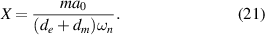
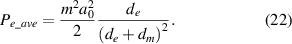
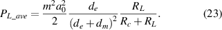
The vibration amplitude and output power at resonant frequency calculated by equations (21 )–( 23) and numerical method are listed in table 6. It can be observed that when the excitation is small enough, the numerical results are in good agreement with the analytical solution of the linear system. Hence, the reliability of numerical method is verified.
Table 6. Comparison of analytical solutions and numerical results.
| Load resistance: RL = Rc Excitation acceleration: a0 = 0.1 mg (1 g = 9.8 m s−2) | ||||||
|---|---|---|---|---|---|---|
| δ–IMO | ωn (Hz) | X (μm) | PL_ave (nW) | |||
| Analytical solution | Numerical results | Analytical solution | Numerical results | Analytical solution | Numerical results | |
| 0.5–25 | 529.93 | 529.96 | 2.95 | 2.71 | 0.162 | 0.138 |
| 0.7–150 | 451.20 | 451.20 | 0.38 | 0.37 | 1.79 × 10⁻² | 1.68 × 10⁻² |
| 1.0–750 | 355.81 | 355.80 | 0.25 | 0.25 | 9.02 × 10⁻³ | 9.23 × 10⁻³ |
3.3. Influence of load resistance
The influences of load resistance to output power are analysed in this section. In this study, η is defined as the ratio of load resistance RL and coil resistance Rc: η = RL/Rc . When η is close to zero, most of the power extracted by coils is consumed by the coil resistance; therefore, the output power on the load is significantly low. Moreover, with the increase in load resistance, the system damping decreases, resulting in the reduction of the total power extracted by coils. Therefore, there is an optimal load resistance matching the coil resistance, which could maximise the output power.
Figure 7 shows the output power varying with resistance ratio for different parameters (δ–IMOs are 0.5 mm–25 μm, 0.5 mm–650 μm, 0.7 mm–150 μm, 1.0 mm–750 μm, separately). It can be observed that for different air gaps, the optimal resistance ratio is also different, which is 1.4, 1.6, 1.0 and 1.0 for 0.5 mm–25 μm, 0.5 mm–650 μm, 0.7 mm–150 μm and 1.0 mm–750 μm, respectively. For the linear system, the optimal load resistance can be derived based on equation (23), as:
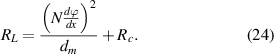

Figure 7. The influence of load resistance to the output power.
Download figure:
Standard image High-resolution imageThe matching load resistance increases with increasing the gradient of the magnetic flux. However, due to the nonlinear characteristics, the specific value and changing rules of optimal load are significantly different from that given by equation (24). This is because in a nonlinear system, the relationship between the vibration amplitude and damping coefficient is not a simple inverse proportional function described by equation (21). However, it is affected by high-order nonlinear components of damping and stiffness curve.
The numerical results also indicate that the sensitivity between optimal load and structural parameters is reduced in this nonlinear system. For example, in the air gap of 0.5 mm, when the resistance ratio is 1, the output power is approximately 5% different from the maximum power. Hence in this study, the resistance ratio of 1.0 is used to perform a unified analysis of the output performance for different air gaps, which could make the load resistance match with the coil resistance in most cases.
3.4. Influence of air gap and initial magnet offset
Figure 8 shows that the output power under 1 g excitation acceleration (1 g = 9.8 m s−2) varies with frequency for different initial magnet offsets, when the air gap ranges from 0.5–1 mm. For the same air gap, the IMO affects the electromagnetic stiffness and flux gradient, which consequently influence the output performance of the VEH. Figure 9 demonstrates the variation in resonant frequency and corresponding output power density with the IMO. Owing to the nonlinear stiffness characteristics of planar springs, the resonant frequency increases slightly with increasing offset near the centre. Away from the centre, the electromagnetic stiffness is rapidly reduced, which gradual decreases the resonant frequency. As for the output power density, a peak is observed at positions of 25, 150, 250, and 750 μm for air gaps of 0.5, 0.7, 0.8, and 1.0 mm, respectively. Reducing the air gap can improve the output power density and simultaneously move the peak position closer to the centre. The maximum output power density is 608.8 μW cm−3 with an air gap of 0.5 mm and initial magnet offset of 25 μm, which is considerably higher than that of the previously published data on VEHs [13, 15–18] (table 7).
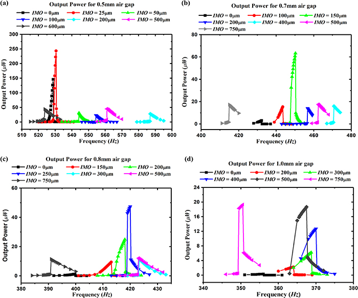
Figure 8. Amplitude–frequency curves of output power for different air gaps: (a) 0.5, (b) 0.7, (c) 0.8, and (d) 1.0 mm.
Download figure:
Standard image High-resolution image
Figure 9. Variation in resonant frequency and resonant output power density with initial magnet offset.
Download figure:
Standard image High-resolution imageTable 7. Comparison of key figures for different harvesters (NPD: normalized power density; 1 g = 9.8 m s-2).
| Reference | V (cm3) | Coils | a0 (g) | P (μW) | fn (Hz) | NPD (μWcm−3 g−2) |
|---|---|---|---|---|---|---|
| [15] | 69.16 | Mechanical winding coils | 0.57 | 5 × 10³ | 54 | 222.52 |
| [13] | 1.61 | MEMS 2D coils | 0.5 | 0.43 | 255 | 10.71 |
| [16] | 0.09 | MEMS 2D coils | 4.5 | 0.82 | 350 | 0.45 |
| [17] | 0.72 | MEMS 2D coils | 1 | 146.3 | 203 | 203.2 |
| [18] | 9.07 | Mechanical winding coils | 0.5 | 224.72 | 6 | 99.08 |
| Proposed | 0.4 | MEMS 3D coils | 1 | 243.52 | 530 | 608.8 |
3.5. Influence of excitation acceleration
Contraposed to a 0.7 mm air gap, the influence of excitation acceleration is investigated, including 0.5 g, 1 g, 2 g, 3 g, 4 g and 5 g (1 g = 9.8 m s-2). The power density and normalized power density (NPD) for 0–250 μm IMO under different excitation accelerations are simulated (figure 10(a)). When the excitation is less than 2 g, the maximum output power is observed at an IMO of 150 μm. For 3 g and 4 g, the optimal IMO increases to 200 μm. However, at 5 g excitation, the output power constantly increases with an increase in the IMO. To normalise the acceleration level, the NPD is calculated (figure 10(b)), which indicates that although the output power increases with excitation acceleration, the NPD reduces when the excitation is enhanced. For a 0.7 mm air gap, the NPD has a peak value of 521.14 μW cm−3 g−2 with a 150 μm IMO and 0.5 g acceleration. The resonant frequency also slightly varies with acceleration, differing from the linear vibration mode. However, when the excitation exceeds 2 g, this variation trend changes at the 150 μm offset, also indicating that the dynamic vibration characteristic is closely related to the excitation level.

Figure 10. (a) Power density and resonant frequency variation with initial magnet offset for different excitation accelerations. (b) Variation in NPD with initial magnet offset for different excitation accelerations (1 g = 9.8 m s-2).
Download figure:
Standard image High-resolution image3.6. Discussion
The influence of air gap, IMO, and excitation can be intuitively determined from the vibration phase portrait. Figure 11 shows the phase locus of different initial magnet offsets under 1 g and 5 g excitations for a 0.7 mm air gap. The cloud chart describes the output power map for each vibration state (x,  ). The cloud chart, calculated using equation (16), is only related to the damping characteristic, de(x). The excitation and IMO simply change the vibration locus in this chart.

Figure 11. Phase portraits for different initial magnet offsets under (a) 1 g and (b) 5 g excitations (1 g = 9.8 m s-2).
Download figure:
Standard image High-resolution image
For 1 g acceleration (figure 11(a)), the maximum instantaneous power (∼ 200 μW) appears at a 150 μm IMO. For IMOs greater than 150 μm, although the magnetic gradient is larger, the phase locus is restricted in a low power region owing to the higher system stiffness, producing lesser electricity. For 5 g acceleration, the vibration phase locus continually increases with an increase in IMO (figure 11(b)), with the maximum instantaneous power occurring at 250 μm.
4. Conclusion
This paper presents a micro EM-VEH based on CMOS-compatible 3D MEMS coils. The magnetic path is closed using a silicon steel sheet inserted in the 3D coils.
In this unique VEH structure, arctangent nonlinear damping and rational stiffness values are used to predict the vibration response and output performance. The VEH performance under different excitation accelerations (0.5–5) for different air gaps (0.5–1 mm) and initial magnet offsets (0–250 μm) is calculated and analysed.
Both the resonant frequency and output power increase with decreasing air gap. As for the initial magnet offset, the resonant frequency first increases with an increase in the IMO near the central position and then reduces, owing to the decrease in the attraction force. The output power has a peak value at a certain offset position, such as 25 μm for a 0.5 mm air gap, 150 μm for 0.7 mm, 250 μm for 0.8 mm, and 750 μm for 1 mm. The maximum output power for a certain air gap increases with the narrowing of the air gap. Under 1 g excitation, the peak output power and power density are 243.52 μW and 608.8 μW cm−3, respectively, when the air gap is 0.5 mm and the magnet installation position is 25 μm, considerably higher than previously published data on MEMS VEHs.
The output power maps and vibration phase portraits are combined to reveal the influence of air gap, IMO, and excitation acceleration. With an increase in the excitation acceleration, the output power increases with a constant air gap and offset. However, the normalised power density reduces. The IMO brings about an asymmetrical characteristic to the system. The enhancement in acceleration level can help the magnet to overcome the stiffness constraint, providing a larger phase locus region and consequently producing a higher output power.
In this study, a systematic modelling and calculation method was proposed for micro electromagnetic vibration energy harvesters comprising a magnetic core structure, and the influence of key parameters was described. These conclusions can be used to guide the design and optimization of vibration energy harvester with similar structure. Moreover, the simulation results indicate that the structure with 3D MEMS coils and magnetic core can significantly enhance the output performance.
Acknowledgments
This work was funded by the National Natural Science Foundation of China (Nos. 51906008 and 51822602) and the High-speed Moving Component Dynamic Tester (2017YFF0107601 and 2017YFF0107604). We would like to thank Editage (www.editage.cn) for English language editing.