
Abstract
We have performed high-level R-matrix scattering calculations to identify and characterise the resonances potentially involved in dissociative electron attachment (DEA) of H2 at around 14.5 eV. DEA experiments (Krishnakumar et al 2018 Nat. Phys.4 149) indicate an asymmetric production of H− around this scattering energy that can only be explained if more than one resonance is involved in the process. The theoretical description of the anion distribution requires accurate data (energy and lifetime) for the resonances involved, currently missing from the literature. We attempt to provide these data for all the resonances identified in the appropriate energy range for bond lengths 1.1 a0 to 4.0 a0. Our resonance results are insufficient to confirm the validity of a simple model of anion yield asymmetry used to reproduce the experimental results.
Export citation and abstract BibTeX RIS

Original content from this work may be used under the terms of the Creative Commons Attribution 4.0 license. Any further distribution of this work must maintain attribution to the author(s) and the title of the work, journal citation and DOI.
1. Introduction
Dissociative electron attachment (DEA) is a process of high significance that takes place when an electron interacts with a molecular target, causing the latter to break into two or more fragments, one of them negatively charged [1]. In it, the incident electron is temporarily attached to the molecule, giving rise to a resonant state characterised by its energy and lifetime (or width). This resonant state can decay either via auto-detachment, leaving the molecule either in its initial (ground) or an excited state (if the target retains some of the kinetic energy of the electron), or via DEA.
H2 is the simplest neutral molecule, and its DEA will produce solely a neutral hydrogen atom and H−. Given the simplicity of the dissociation, one would expect that DEA for this target is well understood. However, velocity slice imaging (VSI) experiments [2] looking at DEA above the H(2l) + H−(1s2) dissociation limit revealed a loss of symmetry in the angular distributions of dissociated H− compared to what would be expected when the dissociation is via a single resonant state. More recent experiments [3] have confirmed this asymmetry. From the measured angular distributions of H−, Krishnakumar et al hypothesised that their experimental results can be explained by considering the dissociation to occur via coherent superposition of a  and a
and a  resonance and calculated an asymmetry for the process using a simple model. The following input data were used in the calculation: a
  potential curve of Eliezer et al [4], the corresponding width derived from the results of Weingartshofer et al [5], a shifted target energy curve for the
  resonance potential energy and a range of likely widths for this latter resonance. Although they managed to obtain values of the asymmetry consistent with their experiment, the approximate data used raise questions about the validity of these calculated results. In addition, Kumar et al [3] invoke the contribution of a third (bound) resonance to explain their measurements.
In this paper, we report resonance potential energy curves and widths for electron scattering from H2 calculated using the R-matrix method [6], focusing on those resonances that could be involved in the DEA asymmetric angular distribution measured by Krishnakumar et al. The R-matrix approach has proven its power to accurately describe both shape and core-excited resonances as a function of bond length for other diatomics [7] as well as for a number of more complex systems [8, 9] at equilibrium geometry. Use of its most recent software implementation, the UKRmol+ suite [10], enables more sophisticated calculations than ever before: Meltzer et al [11] recently performed the most accurate R-matrix calculations of cross sections to date, producing results in excellent agreement with convergent close-coupling and experimental data for H2.
A number of works on DEA of H2 are available in the literature. Experimental results show three peaks in the DEA cross sections for H− production at ∼3.75, ∼10 and ∼14 eV (see Schultz's early review [12]). The two lower energy peaks correspond to DEA into H(1s) + H−(1s2) and are understood [13] to occur, respectively, via a  resonance (with the ground state of H2, X
 , as its parent state) and via a wide
  resonance (with the excited state b
 as its parent). These resonances are shape and core-excited respectively over the inter-nuclear distances around the equilibrium geometry.
Early experimental evidence of the ∼3.75 eV  resonance comes from peaks in the vibrational cross sections obtained by Ramien [14], although little explanation was given for these findings at the time. Later DEA experiments by Schultz and Asundi [15] revealed peaks in the cross section at ∼3.75 eV, which were attributed to the
  resonance described in a theoretical work by Taylor and Harris [16]. Early experimental evidence of the ∼10 eV
  resonance was provided by Schultz [17] and Rapp et al [18], who both obtained DEA cross sections from about 6 to 20 eV. Both experiments showed two peaks, one at ∼10 eV and the other at ∼14 eV, with the ∼10 eV peak attributed in Schultz's review [12] to a
  resonance.
The ∼14 eV peak observed in the absolute cross sections for H− production by Schultz [17] and Rapp et al [18] is described in both papers as arising from dissociation into H(2l) + H−(1s2), with the latter's peak value approximately 50% higher. More recent velocity map imaging (VMI) experiments by Krishnakumar et al [19] provided momentum images of the DEA-produced H− ions as well as absolute cross sections for H− production, with a ∼14 eV peak value close to that obtained by Rapp et al. Both VMI and VSI [20, 21] yield additional information relating to the momentum distributions of the ejected anions, which in turn relates to the symmetry of the resonant state. Neither the above-mentioned papers or Schultz's review [12] attribute the ∼14 eV peak to a particular resonance. Other early experiments [5, 12, 22, 23] looking primarily at vibrational transitions indicate that there is more than one resonance in the vicinity of the higher ∼14 eV peak. In contrast, the resonances leading to DEA at ∼3.75 and ∼10 eV are well isolated and have a single parent state each over the entire range of bond lengths (see below).
One of the first theoretical studies of H2 negative ion resonances was that of Taylor and Harris [16], who described the low lying  resonance used by Schultz and Asundi [15] to explain the peak in their cross sections at ∼3.75 eV. The work of Eliezer et al [4] was more comprehensive and additionally reported three core-excited shape resonances of
  symmetry leading to dissociation into H(2l) + H−(1s2), with parent states c
 , C
, C and EF
 . The more recent work of Stibbe and Tennyson (hereafter S&T) [13] obtained potential energy curves, widths and branching ratios for several resonances using the R-matrix approach and an old diatomic version of the UK Molecular R-matrix Codes [24]. They proposed that Eliezer's resonances are in fact 'manifestations of the same resonance' and described several of the resonances they identified as having more than one parent state. Celiberto et al [25] used S&T's second
  resonance (located at ∼12 eV at equilibrium geometry) only and the local complex potential approximation to calculate the DEA cross section. Although they produced results close to those of Schultz's experiments (seemingly contradicting the later experiment by Krishnakumar et al [19]) the authors themselves state that 'a multichannel formalism for calculating the DEA cross section in the energy region around 14 eV, which includes all the possible resonances with parent states that correlate to the H(n = 2) + H(1s) asymptotic states, would certainly provide a more complete description of the underlying dynamics'. More recently, Laporta et al [26] performed local complex potential approximation calculations of DEA of D2 and reasonably reproduced the peak in the Krishnakumar et al work [19]. These calculations used the resonance data of S&T.
A full theoretical explanation of the asymmetry in the DEA signal around 14 eV measured by Krishnakumar et al [2] requires knowledge of all the resonances that can potentially contribute to the process. A larger number of resonances are expected to be present in the relevant energy range since the H(2l) + H−(1s2) dissociation threshold is ∼0.75 eV below the H(1s) + H(2l) and ∼2.6 eV below the H(1s) + H(3l) dissociation thresholds, onto which a large number of H2 excited states converge. Most of these resonances have received little to no attention so far. Our objective is thus to provide an up-to-date study of the resonances converging to this dissociation limit, including their identification and characterisation, with the hope of providing insight into the recent VSI experiments.
2. Method
2.1. R-matrix theory
Our calculations were performed within the fixed-nuclei approximation using the UKRmol+ software suite [10], versions 2.0.2 and 2.0.1 of the inner and outer region codes respectively [27, 28]. This suite implements the R-matrix method [6, 29], the basis of which is the division of space into inner and outer regions, separated by a spherical surface of radius a, known, respectively, as the R-matrix sphere and radius. The inner region is chosen such that the electronic density of the target states included in the calculation, and that of the molecular orbitals used, is negligible outside it. In the outer region, since the molecular charge density can be considered negligible, the scattering electron is distinguishable from the target electrons and can be modelled as moving under the effect of the molecular potential. In the inner region, the close-coupling approximation is used for the basis set:
Here xn
are the space and spin coordinates of electron n and  is the antisymmetrisation operator. The three functions
  ,
,  and
and  are, respectively, the N-electron target wavefunctions, a set of 'continuum orbitals' describing the projectile and the (N+1-electron) L2 configurations, necessary to describe correlation-polarisation in the inner region. The coefficients aijk
and bik
are obtained from the diagonalisation in the inner region of the sum of the Hamiltonian and Bloch operators, the latter of which is added to restore hermiticity [6].
are, respectively, the N-electron target wavefunctions, a set of 'continuum orbitals' describing the projectile and the (N+1-electron) L2 configurations, necessary to describe correlation-polarisation in the inner region. The coefficients aijk
and bik
are obtained from the diagonalisation in the inner region of the sum of the Hamiltonian and Bloch operators, the latter of which is added to restore hermiticity [6].
In this work, the target wavefunctions are built using configuration interaction (CI). The continuum orbitals, describing the unbound electron in the inner region, are built from B-spline orbitals (BTOs) and are the only single-particle functions that are non-zero on the R-matrix sphere. The UKRmol+ suite is designed to work with orthogonal orbital sets. Therefore, the continuum orbitals must be orthogonalised to the (orthogonal) target molecular orbitals and among themselves. In order to ensure linear independence, the continuum orbitals with eigenvalues of the diagonalised overlap matrix less than a specified threshold (called the deletion threshold) are removed.
The diffuse nature of the H2 target orbitals made BTOs a requirement for this work as they make it possible to use larger R-matrix radii. Finally, the L2 functions, used to model short range correlation and polarisation, are constructed from target orbitals.
Once the Hermitian Hamiltonian in the inner region has been diagonalised and the wavefunctions given by equation (1) and their associated eigenenergies obtained, the R-matrix can be determined from these on the R-matrix sphere.
In the simpler outer region, the N+1 wavefunction can be written as a linear combination of products of target wavefunctions and a single-particle function describing the projectile. The problem then reduces to determining the projectile radial wavefunction  . This leads to the following multi-channel, coupled differential equations:
Here  are the channel momenta and Vij
are the potential terms that connect channel i and j, determined from the target electronic multiple transition moments. The differential equations are solved using a propagation approach [6]. The solutions are then matched to known asymptotic forms, and the K-matrix is obtained. Once the K-matrix has been obtained, scattering quantities such as eigenphase sums, cross sections (from T-matrices, trivially determined from the K-matrices) and time-delays (from S-matrices, similarly trivially obtained) can be easily calculated. Resonance positions and widths can be determined from some of these (see later).
are the channel momenta and Vij
are the potential terms that connect channel i and j, determined from the target electronic multiple transition moments. The differential equations are solved using a propagation approach [6]. The solutions are then matched to known asymptotic forms, and the K-matrix is obtained. Once the K-matrix has been obtained, scattering quantities such as eigenphase sums, cross sections (from T-matrices, trivially determined from the K-matrices) and time-delays (from S-matrices, similarly trivially obtained) can be easily calculated. Resonance positions and widths can be determined from some of these (see later).
2.2. Identification and characterisation of resonances
Resonances are usually identified and characterised by fitting the eigenphase sums [30]. In these cases, the fits are performed using an analytical expression for the resonant contribution and including an approximated non-resonant background expression (e.g. a power series). However, these fittings often fail to detect the resonance, or produce unreliable fits [7, 31], when the background is rapidly varying or when resonances are overlapping or are very close to thresholds.
An alternative method used for the extraction of resonances is the analysis of the time-delay, based on the formulation presented in Smith's work [32]. The time-delay or Q-matrix can be obtained from the S-matrix via:
The eigenvalues of the Q-matrix can, when larger than  , indicate the presence of a resonance, which will appear as a peak of (approximate) Lorentzian shape in the largest eigenvalues of the Q-matrix; sometimes this peak appears across several eigenvalues. Fit of the peak using
allows the determination of the energy, Er
, and width, Γ, of a resonance i ( is a background term). The advantage of this method over fitting to eigenphase sums (or cross sections) is that resonances are much better separated from the background and from each other.
The TIMEDELn [33] package, based on the computation of time-delays, provides the ability to identify and fit resonances across eigenvalues of the Q-matrix. The resonance energies and widths presented in this paper were obtained in a two-step process: first TIMEDELn was run to obtain smooth eigenvalues of the Q-matrix (the program attempts to follow resonant structures across several eigenvalues if needed) and a first set of positions and widths. Secondly, interactive fits using a Python program were performed to improve the accuracy of said fits. The second step was necessary because of the large number of thresholds present in the energy region of interest as well as the presence of non-physical spikes for some of the bond lengths (see below). When a resonance was not significantly affected by its surroundings, the results of both fits were the same.
3. Characteristics of the calculation
H2 is a linear molecule with a centre of inversion and therefore belongs to the D point group. Since the UKRmol+ software suite only supports abelian point groups, the calculations were in the D
 point group with the molecular axis aligned along z.
3.1. Target model
H2, despite being the simplest neutral molecule, has a complex of closely lying and crossing excited states, whose characterisation has been the subject of many studies. A review of the early work can be found in Sharp [34]. From a theoretical perspective, H2 electronic states have been investigated mainly by Kolos, Wolniewicz and collaborators [35–38] and, more recently, by Corongiu et al [39–41] and Nakashima and Nakatsuji [42], who determined accurate energies for a large number of states. Since the latter work involves all of those included in our calculations, we have used it as a benchmark for our target model.
Calculations were performed for a range of bond lengths around the equilibrium geometry. We used the full CI approximation and tested the use of several Dunning [43] type 'cc-pV' basis sets: cc-pVTZ, aug-cc-pwCVTZ, aug-cc-pVQZ-f, aug-cc-pwCV5Z, d-aug-cc-pVDZ, d-aug-cc-pVTZ, d-aug-cc-pVQZ and d-aug-cc-pV5Z. We analysed the agreement of the excitation energies obtained using these bases for the equilibrium geometry. The use of augmented basis sets had a dramatic effect on the description of the electronic states of H2, lowering the excitation thresholds significantly, in better agreement with accurate calculations (e.g. the  state appeared ∼2.5 eV higher than in Nakashima and Nakatsuji's work [42] when non-augmented bases were used). Single augmented bases greatly improved the results, especially for lower excited states, but not to a sufficient degree for the higher energies. Doubly augmented bases produced acceptable results for the higher energy states, in all likelihood due to their more diffuse nature.
When increasing the number of functions describing the valence orbitals, the effect was less significant: there was significant improvement moving from double to triple zeta but not beyond. We deemed triple and above to adequately model the target states of interest and selected the d-aug-cc-pVTZ basis set to obtain the results presented in this paper. (We note that Meltzer et al [11] employed a t-aug-cc-pVTZ basis set that required the use of R-matrix radii of 100 a0. These calculations are too computationally expensive to be carried out for the number of bond lengths investigated in this paper).
The ground state and vertical excitation energies for the equilibrium geometry obtained using the d-aug-cc-pVTZ, d-aug-cc-pVQZ basis sets, along with comparison to Nakashima and Nakatsuji [42], are shown in table 1. We deemed the d-aug-cc-pVTZ basis set to provide a good balance of quality versus computational effort and used it to obtain the results presented in this paper.
Table 1. Absolute ground state and vertical excitation energies of H2, in eV, at the equilibrium bond length 1.4011 a0 calculated with full CI using the basis sets indicated. The results of Nakashima and Nakatsuji [42] are also included. Note that the states are listed in the order in which they appear in our calculations.
| Symmetry | Label | Energy (eV) | ||
|---|---|---|---|---|
| d-aug-cc-pVTZ | d-aug-cc-pVQZ | Nakashima and Nakatsuji [42] | ||
1 
| X | −31.9095 | −31.9427 | −31.9590 |
1 
| b | 10.5788 | 10.5991 | 10.6107 |
1 
| a | 12.5071 | 12.5272 | 12.5368 |
1 
| c | 12.7036 | 12.7198 | 12.7287 |
1 
| B | 12.7229 | 12.7401 | 12.7500 |
2 
| EF | 13.0973 | 13.1154 | 13.1247 |
1 
| C | 13.1973 | 13.2102 | 13.2162 |
2 
| e | 14.4166 | 14.4359 | 14.4432 |
2 
| h | 14.7726 | 14.7948 | 14.8038 |
2 
| B
| 14.8177 | 14.8387 | 14.8478 |
3 
| GK | 14.9450 | 14.9635 | 14.9083 |
1 
| i | 15.0844 | 15.0547 | 14.9143 |
1 
| I | 15.0875 | 15.0574 | 14.9158 |
3 
| g | 15.1734 | 15.1046 | 14.9069 |
4 
| HH | 15.1908 | 15.1140 | 14.9644 |
3 
| m | 15.4804 | 15.4859 | 15.4073 |
3 
| B'' | 15.8532 | 15.8235 | 15.5577 |
2 
| d | 15.9697 | 15.6748 | 14.8450 |
1 
| — | 16.3471 | 16.1929 | 14.9387 |
1 
| — | 16.3599 | 16.2027 | 14.9403 |
2 
| — | 16.7720 | 16.3026 | 14.9858 |
Figure 1 shows the energies of the states of interest for bond lengths R = 1.0 a0 to R = 4.0 a0. It can be seen that our energies agree well with Nakashima and Nakatsuji's results for the states converging on the H(1s) + H(1s) dissociation threshold: the absolute ground state energy at equilibrium geometry is 0.05 eV higher than Nakashima and Nakatsuji's, the lowest excitation energy (for state  ) 0.03 eV higher. For the states converging on H(1s) + H(2l), agreement is also good, with our excitation thresholds at equilibrium geometry 0.03 eV higher, with the exception of the high-energy
  state, which is 0.07 eV higher, and the two
  states, which are 0.17 eV higher. The deviations at equilibrium geometry are approximately carried across the range of bond lengths for all but three of our states converging on H(1s) + H(2l). The h
 and GK
 state deviations significantly increase at higher bond lengths, with a maximum difference of 0.12 eV at R = 3.2 a0 for the
  state and 0.23 eV at R = 2.4 a0 for the GK
 state. Conversely, the description of the
  state, which is 0.07 eV higher than in Nakashima and Nakatsuji's results at equilibrium bond length, improves significantly at the higher bond lengths.
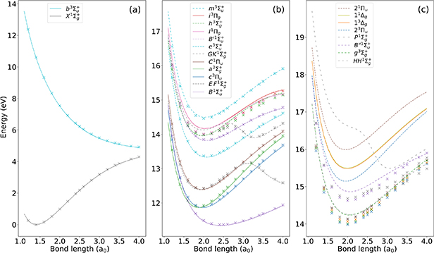
Figure 1. Target state energies for H2 as a function of inter-nuclear separation, calculated with the d-aug-cc-pVTZ basis set (full lines) and those of Nakashima and Nakatsuji [42] (crosses). Energies are shown relative to the ground state at equilibrium geometry and are distributed in the three panels according to their dissociation limit: (a) H(1s) + H(1s); (b) H(1s) + H(2l); and (c) H(1s) + H( 2l). Lines are coloured according to the state symmetry and styled according to the state number.
Download figure:
Standard image High-resolution imageFor states converging on thresholds higher than H(1s) + H(2l), the quality of the results drastically deteriorated, with differences of up to nearly 2 eV in some cases. However, the H(1s) + H(3l) threshold energy is ∼2.5 eV above the H(2l) + H−(1s2) dissociation limit of interest to our study, and as such we deemed these states less likely to be parents of resonances of interest.
3.2. Scattering model
We included 29 D target states listed in table 1 in our calculations; they correspond to 21 states in the D
 point group and include all states dissociating to the H(1s) + H(1s) threshold and those dissociating to H(1s) + H(2l) that are deemed likely to be parent states of resonances involving DEA around 14.5 eV. Tests with 50 target states for the equilibrium geometry showed little difference in the scattering results in the energy region of interest.
The UKRmol+ software suite [10] provides a program (RADDEN) to calculate the orbital amplitudes at the R-matrix boundary and therefore determine the minimum R-matrix radius required to contain the target electronic density. One should consider that the larger the R-matrix radius the more continuum functions (whether GTO or BTO) will be required, which results in longer calculation times. It is thus beneficial to keep the R-matrix radius as small as possible. An R-matrix radius of 40 a0 was necessary to ensure all the target orbitals (for the d-aug-cc-pVTZ basis set) had negligible amplitude at the boundary. The largest value of the probability density of the orbitals at 40 a0 for the d-aug-cc-pVTZ basis sets was  . The benchmark cross section calculations of Meltzer et al [11] used a bigger, more diffuse basis set, t-aug-cc-pVTZ, and required an R-matrix radius of 100 a0; BTOs were used for the continuum description. In those calculations, 98 target states were included in the close-coupling expansion; the computational resource required meant that they were only performed for the equilibrium geometry. To give an idea of how our model compares with theirs, figure 2 shows our cross section for electron excitation into state a
 and that of Meltzer et al: one can see that the size of the cross section is similar in both models but the resonance structure is shifted by around ∼0.2 eV. This difference could be taken to indicate the uncertainty in our calculated positions.

Figure 2. Integral cross section for electronic excitation from the ground state to state a at equilibrium geometry: R = 1.40 a0 in our case and R = 1.448 a0 in Meltzer et al.
Download figure:
Standard image High-resolution imageWe used a BTO-only basis to describe the continuum. This basis was comprised of 30 BTOs of order 9 and partial waves up to l = 6. Increasing the number of BTOs or the number of partial waves above these values made only negligible difference to the scattering results. A deletion threshold of 10−4 was used for the orthogonalisation of the continuum orbitals.
A propagation radius of 200 a0 was sufficient to obtain good scattering results at most bond lengths. However, around 1.9 a0, where both the c and a
and a states and the C
 and GK
 states are very close to one another, as well as around 2.9 a0, where the C
 and GK
 thresholds are also very close to one another, greater propagation radii were required for converged results. In these cases, propagation radii of up to 1100 a0 were used. Nonetheless, our results for these bond lengths still showed the presence of unphysical spikes in the time-delays and cross sections.
4. Results
Our results are presented below for each of the following seven D symmetries:
  ,
,  ,
,  ,
,  ,
,  ,
,  and
and  . No evidence of
  resonances was found in the energy region of interest. Resonance energy curves are shown in this section, while the corresponding widths are presented in figures available elsewhere together with the numerical data (see Data availability statement). The corresponding resonance data from S&T are included in all these figures for comparison. In the case of the resonance energy curves, we have plotted the S&T energies with respect to our target equilibrium ground state energy.
For each of these symmetries, calculations were performed for R from 1.1 a0 to 4.0 a0 in steps of 0.1 a0. The energy range examined for each of the bond lengths was such that all target states dissociating to H(1s) + H(2l) shown in figure 1(b) were included (a range of energies below/above the lowest/highest threshold for these states ensured all resonances associated with them were considered).
The resonance parameters were obtained from the time-delay as discussed in section 2.2. When discussing our results, we make reference to the Lorentzian peak associated with the resonance in the time-delay. Due to the very close proximity of several target states at 1.9 a0 we were not always able to obtain fits to the resonance peaks at this bond length. No attempt was made to fully determine parent states of the resonances via reduced state calculations or any other approach; instead, likely parent states have been inferred from inspection of the resonance energy curves and the neighbouring target states. They should only be taken as indicative.
We note as well that very narrow resonances close to the excitation thresholds are hard to distinguish from threshold effects and may have therefore been missed. In addition, although there are no explicit crossings between resonances of the same symmetry, not all the energy curves can be considered fully adiabatic: in three cases (symmetries  and
and  ) continuation of the resonance is very likely to lead to crossings. This implies that three of the resonance curves may have partial diabatic character.
4.1.
 resonances

Evidence was found of ten resonances of  symmetry likely to converge on the H(1s) + H−(1s2) dissociation limit. Their energy as a function of R is shown in figure 3. Two of these resonances, 1
 and 2
and 2 , are documented in S&T, and the remaining ones are, to our knowledge, undocumented in the current literature.
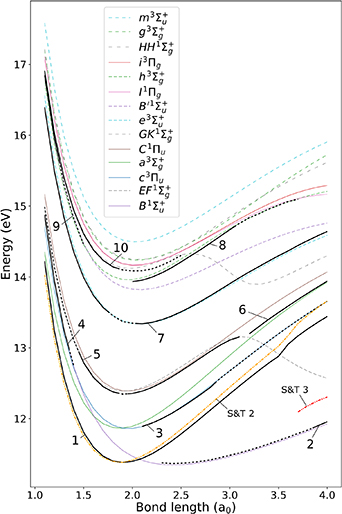
Figure 3.
 resonance (thick black lines: this work; dash-dotted lines: S&T) and target state energies (lighter colour lines) as a function of inter-nuclear separation. The numbers in the figure are referred to in the text to identify the resonances. The included target energy curves are those converging on the H(1s) + H(2l) dissociation threshold shown in figure 1(b) and the m and HH states, which converge on the H(1s) + H(3l) threshold. Dashed black lines are used where TIMEDELn is unable to fit the resonance, so positions from manual inspection of the time-delay eigenvalues are used (no widths were obtained for these bond lengths). The resonance energies obtained by S&T are plotted with colour lines and labelled with 'S&T' and the number used in their paper [13] to identify the resonance.
Download figure:
Standard image High-resolution imageResonance 1 is documented by S&T [13, 44], where it was shown, using reduced state calculations, to have parent states a
 , EF
, EF , c
, c and C
and C . Figure 3 shows our resonance at the lower bond lengths lying below these four parent states. At bond length 1.1 a0 it is relatively wide (
 0.4 eV) and, as a result, the right-hand side of the Lorentzian in the time-delay is truncated by the a
 target state, possibly affecting the quality of the TIMEDELn fit. Resonance 1
 crosses two target states over its detection range: B
 just before 2.1 a0 and EF
 just after ∼3.5 a0. The width decreases for increasing R by about a factor of 25 from 1.1 a0 to the first crossing point at ∼2.1 a0, after which the width begins to rise again. This behaviour is also documented in S&T, although the increase in the width is more noticeable in our results. The second crossing induces a jump both in the width and in the energy curves, although this time the increase in width is smaller in our results than in S&T's. Overall, comparison of our results for this resonance to those of S&T [13] shows an average difference of 0.063 eV in the positions and 0.021 eV in the widths. Our positions are higher throughout, except at 3.9 a0 and 4.0 a0. The widths are higher at the middle bond lengths (2.1 to 3.2 a0) and lower for R outside this range.
Based on S&T's assignment of the B state as its parent, resonance 2
 is core-excited shape in character in the narrow range of bond lengths where it was successfully fitted (3.7–4.0 a0 by S&T; 3.9 and 4.0 a0 in this work). Both calculations show a rapidly decreasing width for increasing bond length in this range, with our results lower in position and higher in width. For smaller R, the maximum in the time-delay is heavily affected by the B
 state threshold and cannot be fitted; the resonance positions here have been obtained from visual inspection. Evidence for the resonance at the lower bond lengths is from the 'tail' of a Lorentzian clearly visible in the time-delay right down to 2.3 a0. For
  2.3 a0 the resonance is likely (based on the previous trend) to be quite wide and is perhaps 'drowned out' by the nearby 1
 resonance. It is therefore possible that this resonance may continue to even smaller bond lengths, since there are visible maxima in the time-delays above the B
 state at bond lengths 1.9, 1.8 and 1.7 a0 and even shorter; this raises the possibility that this and resonance 4
 are actually one resonance. This is quite speculative, and as such we consider the resonance to be convincingly identified between 2.3 and 4.0 a0.
Just above the c target state, between 2.1 to 4.0 a0, a truncated Lorentzian in the time-delay provides evidence of resonance 3
 . This resonance appears likely to be core-excited shape in character with c
 as parent. Between 2.1 and 2.8 a0, just over half of the Lorentzian is present in the time-delay; at higher R even less is visible and, combined with the increasing width, this results in failure to successfully fit the time-delay by 2.9 a0.
At R = 1.1 a0 resonance 4 lies slightly (∼0.007 eV) above the B
 state, its likely parent, making it core-excited shape in character. It then quickly moves closer to the B
 state and is no longer fitted by TIMEDELn by 1.4 a0.
Starting R = 1.1 a0 with a Lorentzian profile significantly truncated by the EF threshold, by 1.5 a0 the 5
 resonance has moved sufficiently away from the threshold for the Lorentzian maximum to be visible and successfully fitted by TIMEDELn. This is a narrow resonance (
 0.008 eV throughout); the width increases slowly until ∼3.1 a0 where it drops and the resonance is 'absorbed' into the EF
 threshold. The resonance is no longer observed for the higher bond lengths. This is likely a Feshbach resonance with EF
 as its main parent state.
Resonance 6 is relatively wide and core-excited shape (assuming a
 is its parent state), first appearing around the R where EF
 drops below the a
 state. It is detected up to 4.0 a0.
Resonance 7 is present below target state e
 (likely its parent state) for R = 1.1 a0 and has a width of ∼0.046 eV. This width changes little until, at ∼1.9 a0, the resonance crosses state e
 and it starts to increase while the resonance moves away from the e
 state. At ∼3.2 a0, just after the GK
 state crosses below the e
 state, there is a small drop in the width. If e
 is assumed to be its parent state, the resonance changes from Feshbach at the lower bond lengths to core-excited shape at the higher ones.
Resonance 8 is first evident at
  2.0 a0, lying between the h
 and B
and B target states. The maximum of the associated Lorentzian in the time-delay is interrupted by the thresholds of both these states, although much more so by the closer h
 . As the bond length increases, state B
 moves away and the resonance narrows, such that by ∼2.8 a0 its Lorentzian is nearly fully visible. As the bond length increases further, the resonance begins to move closer to the h
 state so that only a Lorentzian 'tail' is present up to at least 3.7 a0. State h
 appears to be the parent of the resonance, making it Feshbach in character.
Resonance 9 is fitted only for the two lowest bond lengths, where it is located below B
 , its likely parent state, and is thus Feshbach in character. At 1.5 a0 it becomes very hard to distinguish due to the large number of surrounding target states. There is some inconclusive evidence in the time-delays that the resonance follows its parent at higher R after the crossing of the B
 and h
and h target states; Lorentzian 'tails' can be observed around the B
 state up until ∼2.8 a0.
Resonance 10 is located below the GK
 target state (its likely parent) up until ∼2.5 a0, at which point the GK energy curve turns downwards due to an avoided crossing with state EF
 . The nearby I, i and h states, as well as resonance 8
 make it difficult to determine whether or not the resonance continues to higher bond lengths.Resonance
  is likely Feshbach with GK
 as parent.
4.2.
resonances

Only one  resonance was detected with confidence. This is a relatively wide resonance (∼0.36 eV) that appears below the m
 target state and above the g
 and HH
 states (see figure 4). After R = 1.8 a0 it is not possible for TIMEDELn to fit the resonance: no widths were obtained for larger bond lengths. After
  3.3 a0 the resonance is barely discernible from the background.
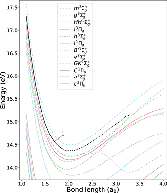
Figure 4.
 resonance (thick black lines) and target state energies (coloured lines) as a function of inter-nuclear separation. Other details as in figure 3.
Download figure:
Standard image High-resolution image4.3.
resonances

We have confidently identified four resonances of  symmetry converging to the H(2l) + H−(1s2) dissociation limit. These are shown in figure 5.

Figure 5.
 resonance (thick black lines) and target state energies (coloured lines) as a function of inter-nuclear separation. Other details as in figure 3.
Download figure:
Standard image High-resolution imageResonance 1 is observed between 1.5 and 4.0 a0. Although the Lorentzian in the time-delay is well defined for the first bond lengths, for R = 1.7, 1.8 a0 the proximity of the a
 threshold and the increase in resonance width (by 1.8 a0 ∼5× the width at 1.5 a0) mean that reliable fits could not be obtained. For higher R the dramatic widening of the resonance means the thresholds for the B
 state increasingly affect its profile in the time-delay: by 2.2 a0, we were unable to produce reliable fits and report only estimates of the position. The resonance is likely core-excited shape in character with
  as parent.
At the initial bond length of 1.1 a0, resonance 2 is below state e
 , its likely parent state, making it Feshbach in character. By R = 1.3 a0 the resonance has become so close to the threshold that only a 'tail' is present in the time-delays, preventing fits from being obtained for the remainder of the R. The 'tail' appears to shift from being predominately on the low-energy side below 1.5 a0 to the high-energy side above this R, perhaps indicating a change in character from Feshbach to core-excited shape.
Resonance 3 is initially detected at 1.1 a0, below target state B
 . For increasing R it both narrows and moves closer to state B
 , until at 2.6 a0 it can no longer be reliably fitted. There is no convincing evidence of the resonance for
  2.8 a0, when the GK
 target state drops below
  . Although the resonance curve does not obviously follow that of state B
 , this is a possible parent state making the resonance Feshbach.
Resonance 4 follows closely the GK
 target state over the range of bond lengths where it is detected. This state has little effect on the resonance profile in the time-delay (that is neither skewed nor truncated by it). The resonance has several target states, B
 and h
and h at the lower R and i
 and I
and I at the higher R, very close to it, making it impossible to assign it a specific parent state. The width increases from ∼0.11 eV at 1.1 a0 to a maximum of ∼0.14 eV at 1.6 a0 and then decreases again to ∼0.11 eV at 2.0 a0. At higher R, up to around 2.5 a0 there is still some evidence of the resonance in the form of Lorentzian tails; however, it is impossible to provide an accurate estimate of the resonance position.
In addition to these  resonances, there is some evidence of other resonances in the time-delay, in the form of Lorentzian tails: firstly, around the c
 and C
and C target states over nearly the entire range of R in both cases; also above the a
 target state running from 2.0 to 4.0 a0; finally, just above the GK
 (but below the e
 ) target state from 3.3 to 4.0 a0 and around the C
 state over the entire range of R.
4.4.
resonances

The energy curves for the resonances of  symmetry are plotted in figure 6. Resonance 1
 , located between the a
 and c
and c target states, is clearly identifiable in the time-delay. Its energy closely follows that of state c
 , making it potentially its parent and the resonance Feshbach in character. As the R increases from 1.1 a0, the resonance narrows rapidly and the a
 and c
and c thresholds get closer; however, the narrowing occurs at a greater rate (than the encroachment of the targets) and by ∼1.7 a0 nearly the entire Lorentzian-like form is visible in the time-delay, with little interruption from the surrounding target states. After the
  and c
and c states cross, it is no longer possible to follow the resonance with any certainty. It is therefore not possible to ascertain whether 2
 is a continuation of this resonance.

Figure 6.
 resonance (thick black lines) and target state energies (coloured lines) as a function of inter-nuclear separation. Other details as in figure 3. Note that, to aid the reader, we have used dashes at higher bond lengths for S&T 11 where S&T actually report single R values.
Download figure:
Standard image High-resolution imageResonance 2 is first evident at R = 2.1 a0 (some inconclusive evidence is visible at 2.0 a0 and even smaller R where the crossing of the a
 and c
and c target states complicates the time-delay). The resonance lies above the c
 state and is therefore likely core-excited shape in character. As R increases, the resonance moves away from its parent, first widening and then, after ∼3.1 a0, narrowing. At ∼3.4 a0, the EF
 state crosses both the resonance and state c
 , and the resonance again begins to widen.
Resonance 3 is sandwiched between states EF
 and C
and C . Similarly to resonance 1
 , it narrows rapidly as R increases and appears to disappear after the above-mentioned states cross.
Resonance 4 is a higher energy, relatively wide, resonance. It was clearly evident in the time-delays from 2.0 a0 up until 2.6 a0. It may continue to the lower bond lengths but the large number of target states in close proximity made this impossible to ascertain with confidence. The energy curve of this resonance behaves quite differently to those of the nearby target states but more similarly to those of the h
 or m
or m states; we therefore assume that these latter are the more likely parent states.
The highest energy and widest resonance, 5 , sits just above the g
 , HH
, HH and i
and i states at the lower bond lengths (only the latter converges on to the H(2l) + H−(1s2) limit). The resonance moves slowly away from these states with increasing R. By R = 1.9 a0 the Lorentzian is barely discernible in the time-delay and, as such, widths cannot be provided. The resonance does not have obvious parentage.
In addition to the resonances reported, inconclusive evidence (a Lorentzian 'tail' on the high-energy side in the time-delay) of a further resonance above the C target state running from
  2.1 a0 to at least 3.2 a0 is visible.
4.5.
resonances

The energy curves of the nine identified and characterised resonances of  symmetry are shown in figure 7. Resonance 1
 is documented in S&T. The remaining eight resonances are, to our knowledge, undocumented in the current literature. S&T describe another
  resonance, that follows the b
 target state, which we also saw evidence of in our time-delays. However, since the b
 target state dissociates into H(1s) + H(1s), it is outside the scope of this study and has been excluded from figure 7.

Figure 7.
 resonance (thick black lines) and target state energies (coloured lines) as a function of inter-nuclear separation. Other details as in figure 3.
Download figure:
Standard image High-resolution imageResonance 1 is likely Feshbach in character and was identified for the whole range of R, although at 1.0 a0 it is too close to state a
 for TIMEDELn to be fitted. However, evidence of this resonance is clear in the eigenphase sum, with a jump of approximately π around the a
 threshold. As R increases, the energy gap between the 1
 resonance and state a
 increases, and the width rapidly decreases. At
  1.6 a0, the B
 state drops below the a
 state and approaches the resonance: by 2.5 a0 the resonance is nearly on top of this state and its width has decreased by a factor of ten. From this bond length up until R = 3.8 a0, TIMEDELn fails to fit the resonance, although the tails of the Lorentzian profile are clearly visible in the time-delay. Successful fits are not obtained again until 3.8 a0, at which point the resonance is moving away from the B
 state and its width is increasing with R.
As mentioned, the 1 resonance has previously been documented by S&T and, as such, provided a useful comparison for our calculations. The results agree well; our positions (relative to the ground state equilibrium energy) are slightly higher for
  2.9 a0 and slightly lower for
  2.9 a0. The maximum difference is ∼0.12 eV, although this is much smaller for the central bond lengths, with an average difference of ∼0.02 eV. The widths also follow the same trends, but the differences are higher: approximately −40% and +7% (our results relative to S&T) for the biggest and smallest values of the widths, respectively. We note that S&T experienced the same issues when fitting their time-delays for this resonance at the central bond lengths. S&T [13, 44] have shown, using reduced state calculations, that the parentage is shared by both B
 and a
and a states, with B
 dominating at higher R and a
 at lower ones.
Between 2.0 and 2.8 a0, sandwiched by the C (above) and EF
 (below) states, we found evidence of the relatively narrow (∼0.01–0.02 eV) resonance 2
 . Outside this range (where
  is below the C
 state) there was no definitive evidence of the resonance: Lorentzian tails can be observed in the time-delay near the EF
 threshold until this state crosses below a
 , but we deemed this to be insufficient evidence.
Resonance 3 is evident from the time-delay from 3.4 to 4.0 a0. The resonance is wide enough such that the associated Lorentzian in the time-delay is truncated by the nearby GK
 state, which is its likely parent. After the avoided crossing between the EF
 and GK
 states the resonance disappears.
The e target state is associated with (and is the likely parent of) two resonances at lower R. Resonance 4
 is narrower, with a width decreasing from ∼0.035 eV at 1.1 a0 to ∼0.02 eV at 1.4 a0. After 1.4 a0 the resonance moves closer to the e
 target state, and no TIMEDELn fits were obtained (although a Lorentzian 'tail' is present throughout the remainder of the R on the low-energy side of the e
 threshold). The resonance appears to be Feshbach in character, with e
 as its parent state. The second resonance, 5
 , appears to be core-excited shape and is wider: ∼0.05 eV at 1.1 a0, increasing to ∼0.24 eV at 1.6 a0. Shortly after 1.6 a0, as the resonance widens, evidence of its presence gradually diminishes until it is no longer discernible from the background.
Resonance 6 displays a clear Lorentzian peak in the time-delay at 1.5 a0. Below this bond length, evidence of this resonance is from a Lorentzian 'tail' on the high-energy side of the B
 threshold. The resonance follows this target state, sitting above it, until the GK
 state crosses them both from above, after which no evidence of the resonance can be found in the time-delay. The resonance is likely core-excited shape in character. Both the resonance and its parent are crossed by the h
 target state
  1.55 a0 without affecting the resonant Lorentzian peak in the time-delay. The resonance width increases from ∼0.04 eV at 1.5 a0 to a maximum of ∼0.13 eV at 2.6 a0 before decreasing again.
In addition to the resonances mentioned, there is some evidence in the time-delay of other possible resonances of this symmetry: (i) above the threshold of state a over the entire range of R (a Lorentzian 'tail' is seen); (ii) running above the I
 and i
and i thresholds and below the g
 and HH
 from 1.1 to ∼2.0 a0 we observe the peak of what looks like a resonance that is much wider than the energy difference between thresholds; (iii) from 1.1 to ∼2.9 a0 there is a Lorentzian 'tail' on the low-energy side of the B
 threshold.
4.6.
resonances

There was no conclusive evidence of any resonances of  symmetry within the investigated R and energy ranges. However, there was some indication of possible resonances in the time-delays that could not be fitted: above the B
 and c
and c target states between 1.1 and ∼1.7 a0, above the a
 state between ∼1.7 and at least 3.1 a0 and also above the EF
 state from ∼1.7 to ∼2.8 a0. Some further indication of resonances in the shape of tails on the higher energy side of the I
 and i
and i thresholds was also visible.
4.7.
resonances

We found strong evidence of seven resonances of  symmetry. Their energies are shown in figure 8.
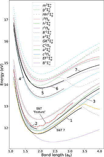
Figure 8.
 resonance (thick black lines) and target state energies (coloured lines) as a function of inter-nuclear separation.
Other details as in figure 3.
resonance (thick black lines) and target state energies (coloured lines) as a function of inter-nuclear separation.
Other details as in figure 3.
Download figure:
Standard image High-resolution imageResonance 1 , which was also documented by S&T, has a distinct Lorentzian maximum in the time-delays between R = 1.2 a0 and R = 3.4 a0. At 1.1 a0 the Lorentzian is truncated by the a
 threshold, and no reliable fits could be obtained. For the higher R, up until 3.4 a0, the resonance is sufficiently far from the surrounding thresholds to allow good fits with provision of reliable widths. The width at 1.2 a0 is ∼0.027 eV, which decreases to a minimum at ∼1.8 a0 of ∼0.0076 eV, just after the B
 state drops below the resonance. After this, the width increases to ∼0.1 eV at 3.4 a0.
Agreement with the results of S&T for this resonance is poorer than for the  and
and  ones. Although the trends in the width are roughly the same, with a minimum at ∼1.8 a0, there is significant difference in the positions and the widths. Our widths vary more smoothly with bond length than those reported by S&T: a large number of 'jags' in their widths are not present in our results. Our relative positions are higher throughout, with an average absolute difference of ∼0.077 eV. For the widths, the average absolute/relative difference is ∼0.013 eV/55%, with our results higher throughout, except at the lowest bond lengths. A possible source for the differences between our results and those of S&T is the likely better description of polarisation effects in our calculations.
S&T assign a , c
, c and EF
 as parent states of this resonance. Our results also suggest the a
 and c
and c states as parents below 3.4 a0: the resonance sits below both of these states throughout, immediately below the a
 state at lower bond lengths and immediately below the c
 state at the higher ones (the a
 and c
and c
 states cross one another at ∼1.9 a0), making the resonance Feshbach in character.
Evidence of a relatively wide ( 0.2 eV), core-excited shape resonance, 2
 , was found above the c
 target state (its likely parent) at the lower bond lengths. Reliable fits were only obtained for 1.7, 1.8 and 1.9 a0. For shorter bond lengths, although a maximum of the Lorentzian was sometimes visible in the time-delay, attempted fits were too poor to provide reliable values for the position and width. Below 1.4 a0 the Lorentzian maximum was not visible in the time-delays due to truncation by the c
 target state. The resonance is no longer present in our data after the a
 target state crosses the c
 state from below, at ∼1.9 a0.
Although relatively wide (0.1–0.2 eV), resonance 3 is sufficiently far from the surrounding thresholds at 4.0 a0 to manifest as a nearly complete Lorentzian in the time-delays. However, as the bond length shortens, the resonance gradually approaches the a
 threshold from below, until at R = 2.5 a0, the maximum is no longer discernible in the time-delay profile and only a 'tail' on the low-energy side of the a
 target state indicates its presence. It may also be linked to a (seemingly separate) 'tail' on the high-energy side of a
 running from at least 1.5 a0 (below our cut-off for this resonance) up until 1.7 a0. It is hard to know for sure whether this high-energy 'tail' is connected to 3
 ; if it is, this would extend the bond length range of 3
 to potentially the whole range of R investigated. The width, throughout the range where we obtained fits, increases from ∼0.14 eV at 2.6 a0 to a maximum value of ∼0.19 eV at 3.3 a0 (just after the resonance crosses the descending EF
 state). After this, the width decreases to a value of ∼0.1 eV at 4.0 a0. For most of the bond length range, 3
 appears to be Feshbach in character with the a
 target state as parent.
Although the Lorentzian peak in the time-delay associated with resonance 4 is truncated on the low-energy side, it is well fitted at the initial bond length of 1.1 a0, which yields a width of ∼0.05 eV. However, as R increases, the resonance rapidly widens to ∼0.22 eV at 1.4 a0, the final fitted bond length. Above this bond length, although the time-delay profile has a distinct maximum, it is asymmetrically skewed by the (lower lying) e
 target state, and achieving reliable fits is impossible. However, it is clear from visual inspection of the time-delays that the resonance continues to widen, such that by 2.8 a0 it is barely discernible from the non-resonant background. It is highly likely that the resonance is core-excited shape in character with e
 as its parent state.
The resonance behaviour around the h and B
and B target states is impossible to decipher with certainty, especially around R = 1.5 and 1.6 a0 where the two states cross. Resonance 5
 initially appears, at 1.1 a0, above the h
 state, where its width is much higher than that of resonances 4
 and 6
and 6 . In the time-delay, the associated Lorentzian is 'tail-less' due to the influence of these two surrounding resonances. The central section of the Lorentzian, however, can be fitted well, which provided a width of ∼0.17 eV at 1.1 a0. After this, up to the final fitted bond length, 1.6 a0, the resonance narrows slightly (to ∼0.17 eV at 1.6 a0). For R = 1.1, 1.2 a0 resonance 5
 is located above the h
 and below the B
 target states. At around 1.3 a0 it moves below the h
 state where it remains for increasing bond length. By ∼1.6 a0 the h
 target state crosses the B
 state from below and continues to move away from the resonance. The resonance appears (from visual inspection of the time-delays) to continue to the higher bond lengths as a 'tail' on the low-energy side of the B
 state that is present even as the h
 and B
and B states move apart from one another. By 2.2 a0 the 'tail' is barely discernible. We thus consider the 5
 resonance as Feshbach in character with the B
 state as parent, although there may be some contribution to parentage from the h
 state at the lower bond lengths.
Resonance 6 is detected at 1.1 a0 as a relatively narrow (∼0.017 eV) resonance, truncated below its maximum by the B
 target state. As R increases, the resonance appears to widen, to ∼0.09 eV at 1.6 a0 (just after the B
 and h
and h states cross). At 1.7 a0, we were unable to get a reliable fit; however, for 1.7 a
 2.8 a0, acceptable fits were obtained. After 1.7 a0 there is an initial (quite dramatic) drop in the width to ∼0.06 eV, after which the width increases to a maximum of ∼0.11 eV at 2.6 a0. Above 2.6 a0, where the avoided crossing between states GK
 and EF
 starts to play a role, the resonance appears to narrow.
Resonance 7 becomes apparent in the time-delays just after the GK
 state crosses below the B
 state at 2.9 a0. As R increases and the GK
 state moves away from it, the resonance narrows quickly to a minimum at ∼3.1 a0 and then slowly widens over the remaining R, so that at 4.0 a0 it has a width of ∼0.43 eV. This is the widest of all the
  included in figure 8. It is likely that this resonance has state B
 as parent and is core-excited shape in character. There is a possibility that 7
 is a continuation of resonance 6
 , but the complexity of the time-delays around the bond lengths where the GK target state crosses both the resonance and the B
 target states make this difficult to determine with reasonable certainty.
In addition to the resonances documented above, there were several tails around many of the target states: (i) on the high-energy side of state h just after it crosses the B
 state, present up until at least 3.0 a0 after which the close proximity of the I
 and i
and i thresholds make the 'tail' impossible to discern confidently; (ii) on the low-energy side of the C
 target state from ∼1.9 a0, where this state crosses below the EF
 state, to 4.0 a0; this 'tail' has relatively large time-delay values; (iii) on the high-energy side of the EF
 state from 1.0 a0 to before it crosses above the C
 state at ∼1.9 a0; (iv) a smaller tail above the GK
 target state, which is most significant after GK
 crosses under the B
 state.
4.8.
resonances

Figure 9 shows the two resonances of  symmetry we have identified. Both were detected across the entire range of R and are core-excited shape in character: the parents are the e
 state for 1
 and the B
 state for 2
 . The widths of both resonances increase for increasing R, with 2
 the narrower of the two throughout.
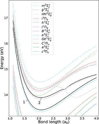
Figure 9.
 resonance (thick black lines) and target state energies (coloured lines) as a function of inter-nuclear separation.
Other details as in figure 3.
resonance (thick black lines) and target state energies (coloured lines) as a function of inter-nuclear separation.
Other details as in figure 3.
Download figure:
Standard image High-resolution imageWe were unable to fit resonance 2 at R = 2.9 a0, although a Lorentzian 'tail' was still visible in the time-delays. There is a small step in the width of resonance 1
 at 3.7 a0, very likely related to changes in the quality of the fit; at
  3.7 a0 the time-delay eigenvalue associated with this resonance drops abruptly at the B
 threshold, and for higher R it cleanly crosses the threshold. This allowed more data points to be provided to the fit routines at the higher R.
In addition to these resonances, we found some potential evidence of other resonances of  symmetry: above the C
 threshold across all R, above c
 at lower R and above a
 at the higher R.
5. Discussion: link to DEA at around 14.5 eV
The VSI experiments of Krishnakumar et al [2] revealed an asymmetry in the momentum distributions of H− for scattering energies 14.5, 15 and 15.5 eV. In their paper, the experimental asymmetry is quantified using:
where  and
and  are, respectively, the signal strength in the forward and backward directions (with respect to the incident electron beam). The measured values for η vary from −0.19±0.02 at 14.5 eV to −0.17 at 15.0 eV and −0.12±0.02 at 15.5 eV, indicating a stronger anion signal in the backward direction at the three energies.
Krishnakumar et al assumed that two interacting resonances, of  and
and  symmetry, are responsible for the DEA and calculated η using the following expression:
Here E is the scattering energy and µ the reduced mass of the system. In addition, the theoretical expression depends on: the energy curve of each resonance as a function of bond length,  and
and  , the average auto-detachment lifetime of each resonance, τu
and τg
, the 'dissociation time' associated with each resonance, tu
and tg
, and the bond length at which electron capture takes place, Rc.
, the average auto-detachment lifetime of each resonance, τu
and τg
, the 'dissociation time' associated with each resonance, tu
and tg
, and the bond length at which electron capture takes place, Rc.
As input to their model, Krishnakumar et al used for the  curve that of one of the two closely lying
  resonances reported in Eliezer's early work [4] (they do not indicate which one), and τg
= 8 fs (taken from [5]). For
resonances reported in Eliezer's early work [4] (they do not indicate which one), and τg
= 8 fs (taken from [5]). For  they used the H2 B
 and C
and C target state energies shifted by an unspecified amount, which we assumed to be the difference between the H(2l) + H−(1s2) and H(1s) + H(2l) asymptotic energies. Both curves can be seen in figure 10. The asymmetry η was obtained for several τu
ranging from 1 to 50 fs and compared with experiment. The closest match to their VSI experiments was obtained using the C
target state energies shifted by an unspecified amount, which we assumed to be the difference between the H(2l) + H−(1s2) and H(1s) + H(2l) asymptotic energies. Both curves can be seen in figure 10. The asymmetry η was obtained for several τu
ranging from 1 to 50 fs and compared with experiment. The closest match to their VSI experiments was obtained using the C shifted target state with
  3.5 fs or
  25 fs.
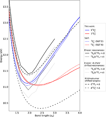
Figure 10. Potential energy curves of the resonances considered when attempting to calculate the asymmetry parameter. In addition to the resonances calculated in this work (coloured full lines), data from Stibbe and Tennyson [13] (coloured dotted lines), Eliezer's data for the relevant  resonances [4], both original (black full and dotted lines) and shifted by 0.25 eV (grey lines), and those used by Krishnakumar et al [2] for the
  state (dashed lines) are also included. All resonance energies are relative to the (explicit or implicit) target ground state energy in the respective works.
Download figure:
Standard image High-resolution image
Assuming a 25 fs dissociation time for both resonances and using the lower energy  (
( ) resonance reported in [4] shifted down by 0.25 eV, we came closest to reproducing Krishnakumar et al's calculated values of η. The 0.25 eV shift applied to the Eliezer resonances was proposed in an early review by Schulz [12] but not mentioned by Krishnakumar et al.
These input data, however, are not consistent with our calculated resonances, as can be clearly seen in figure 10; nor are they consistent with the data from S&T, which are reasonably close to our results. For the  resonance, both the unshifted
  and the shifted
  energy curves are in reasonable agreement with ours, but it is the shifted
 resonance that produces better agreement with Krishnakumar et al's experimental η when we perform the calculation (see above). However, the shifted potential curve is significantly lower in energy than that of our resonance (although the shape of both is not too dissimilar). For the
  resonance, the shifted C
 and B
and B target state energies do not coincide with any resonance of
  or other symmetry obtained in this work. The shifted B
 target state is between 0.5 and 0.7 eV from any calculated resonance of
  symmetry for all bond lengths above ∼1.9 a0. The shifted C
 target state is closer to the nearest
  resonance than the shifted B
 state up until ∼2.8 a0. What is more, our resonance curves cross near 2.0 a0, whereas the curves employed by Krishnakumar do not. The
  lifetime of 8 fs is different to our calculated values: our bond length averaged lifetime is 15 fs and 9.4 fs at equilibrium bond length (that of S&T is 17 fs). Our averaged auto-detachment lifetime for the
  resonance is 31 fs, within the range of values tested by Krishnakumar et al.
The above discussion indicates an inconsistency between the data used by Krishnakumar et al and the resonance data we obtained from our calculations. Attempts to reproduce the observed η using our calculated resonance positions and average lifetimes and equation (6) were unsuccessful. The more significant problem is the high sensitivity of the asymmetry to the resonance potential curves. The 'phase' of η (δ in equation (6)) depends on the potential energy curves of the resonances and the inter-nuclear separation for which the electron capture takes place; for the latter we have assumed the equilibrium bond length. It is this phase that determines the sign of the calculated asymmetry at a given scattering energy, i.e. whether the anion signal is stronger in the forward or backward direction, or symmetric. In order to use equation (6), a significant extrapolation of our calculated data was required. This extrapolation was numerically not very stable, with small changes resulting in quite large changes to the calculated η and therefore to the sign of the asymmetry and the energy at which it changed. In other words, a given extrapolation can lead, for example, to positive asymmetry parameters in the 14.5–15.5 eV range while another can lead to a parameter that changes from negative to positive in this interval. We note that the short cut-off point for the bond length in our calculations also affected the number of widths available for determining the average values of τg and τu .
The 'amplitude' of η (at
in equation (6)) depends only on the auto-ionisation and dissociation times and provides upper and lower bounds to it. Our calculated values for this amplitude using our data are ∼50% bigger than those obtained using the data we assume Krishnakumar et al used (and  25–30 fs), but they are consistent with the measured asymmetries. We also unsuccessfully attempted to reproduce the η using our 7
 and 4
and 4 resonances.
6. Conclusion
Potential energy curves and corresponding widths have been obtained for 35 resonances formed during electron scattering from H2 around the energy of the H(1s) + H(2l) dissociation limit (∼12–16 eV at equilibrium geometry) over the H–H bond length range of 1.1 to 4.0 a0. The time-delay was used for the identification and characterisation of the resonances. We found that this method provided good results for reasonable computational resource, with the main benefit coming from the separation of the resonances across the time-delay eigenvalues. The limitations encountered when using this approach were mostly related to the large number of target thresholds in the energy region of interest and the fact that many resonances are close enough to these thresholds for their associated Lorentzian peak in the time-delay to be truncated or otherwise deformed by their presence. The majority of the resonances are, to our knowledge, identified and characterised for the first time, although several of the lower energy ones were previously documented by S&T. The resonance spectrum that emerges is quite complex.
The uncertainty in the calculated asymmetry makes it impossible to provide a definite conclusion as to whether our resonance data are consistent with the asymmetry η quantified by Krishnakumar et al. The phase of η, which determines the forward/backward asymmetry, is extremely sensitive to the shape of the resonances' potential energy curves: in our case large extrapolations were required, leading to the significant uncertainty in the calculated η. Our resonance energy curves, in particular that of  , are very different to those used by Krishnakumar et al in their calculation of η. Nonetheless, if we were able to accurately continue our resonance curves to larger bond lengths, given the periodic nature of the phase, it would be possible for both our and their resonance data to produce η that match the experiments in terms of their sign. The amplitude, that gives the size of η, can be 'fitted' by choosing the dissociation times which Krishnakumar et al do not provide. Our average lifetimes for the resonances are not too different to those employed by Krishnakumar et al: given the uncertainty in the dissociation times, the amplitude of the measured asymmetry would be relatively straightforward to replicate.
Although interference between two resonant states is the simplest and therefore most elegant explanation for the asymmetry, the resonance data provided in this paper are insufficient to support this conclusion due to the sensitivity to the resonance potential curves of the expression used to calculate η. This opens the possibility that a mechanism based on two interfering Σ resonances of opposite parity does not actually account for the full process and that three (as proposed by Kumar et al) or more resonances are involved. Our calculations show that there are a number of resonances in the appropriate energy region that could contribute to the DEA process. Resonance 7 could be the third resonance that Kumar et al invoke to explain their measurements, but there is also at least one bound
  resonance accessible at 14 eV. Proper nuclear dynamics calculations are needed to confirm the origin of the anion signal asymmetry in DEA to H2 at ∼14.5 eV. Further calculations of these high lying resonances, particularly extending the range of bond lengths studied, would help with this accurate modelling of DEA. Alternatively, the vibrational–electronic molecular convergent close-coupling (MCCC) approach that includes the contribution of resonance states without the need to separately calculate their position and width [45] could be further developed to describe DEA.
Acknowledgments
We acknowledge helpful discussions about resonance modelling and identification with Drs Zdeněk Mašín and Tom Meltzer. In addition, J D G acknowledges support from the UK-AMOR consortium (EP/R029342/1).
Data availability statement
The data that support the findings of this study are openly available at the following URL/DOI: https://ordo.open.ac.uk/articles/dataset/Calculated_energy_and_width_for_resonances_in_electron_H_sub_2_sub_collisions/24148200 [46]. In addition, the widths for all the resonances discussed are also provided in the repository together with figures comparing them to the widths from S&T.