Wigner time delay in atomic photoionization

In this section, we follow closely the work of Kheifets and Ivanov (2010). We consider an atom exposed to a short burst of ionizing radiation. For simplicity, we restrict ourselves to the single active electron (SAE) approximation. This approximation will be relaxed in section 4.3 where we consider multiple ionization processes. For not very strong field intensities, one can use the perturbation theory and expand the time evolving EWP on the basis of scattering states

$$\begin{align} \Phi(\boldsymbol{r},t)= \sum_L \int d^3k \ a_{\boldsymbol{k} L}(t) \chi_{\boldsymbol{k} L}(\boldsymbol{r}) e^{-i E_k t} \ . \end{align} \tag{ 1 }$$

This basis is defined according to equation (136.5) and (c.11) of Landau and Lifshitz (1985):

$$\begin{align} \chi_{\boldsymbol{k} L}(\boldsymbol{r}) = {2\pi\over k} \ i^l e^{-i\delta_l(k)} R_{kl}(r) Y_L^{\,*}(\hat{\boldsymbol{k}}) Y_L(\hat{\boldsymbol{r}}) \ \ , \ \ L\equiv\{l,m\}. \end{align} \tag{ 2 }$$

The asymptotics of the radial orbital $R_{kl}(r)$ is given by equation (36.23)

$$\begin{align} R_{kl}(r\to\infty)\simeq {2\over r} \sin\left(kr+{1\over k}\log\,2kr-{l\pi\over2}+\delta_l\right) \ . \end{align} \tag{ 3 }$$

After termination of the pulse at $t\gt T_1$, the expansion coefficients in equation (1) are expressed as

$$\begin{align} a_{\boldsymbol{k} L}(t>T_1) & =-i \int\limits_{-\infty}^{\,\infty} \langle \chi_{\boldsymbol{k} L}|z|\phi_i\rangle e^{i(E_k-E_i)\tau} {\cal E}(\tau)\ d\tau \ \nonumber\\ & = -i \langle \chi_{\boldsymbol{k} L}|z|\phi_i\rangle \ \tilde{\cal E}(E_k-E_i) \ . \end{align} \tag{ 4 }$$

Here we extended the integration limits outside the pulse duration and wrote the dipole matrix element $\langle \chi_{k\lambda}|z|\phi_i\rangle$ in the length gauge. By separating the angular and radial integration, we can present this matrix element in the reduced form

$$\begin{align} \langle \chi_{kL}|z|\phi_i\rangle \propto C^{lm}_{10\,l_im_i} d_\lambda(k) \ , \end{align} \tag{ 5 }$$

where $C^{lm}_{10\,l_im_i}$ is the Clebsch–Gordan coefficient, $\lambda\equiv L,l_i$ and

$$\begin{align} d_\lambda(k) = \sqrt{2l_i+1} \ C^{l0}_{10\,l_i0} \int r^2dr \, R_{kl}(r)\,r\,R_{n_il_i}(r) \ , \end{align} \tag{ 6 }$$

which is a real quantity. With this definition, we can write

$$\begin{align} a_{kL}\propto-i\,d_\lambda(k) \tilde {\cal E}(E_k-E_i) \ \ , \ \ \tilde {\cal E}(\omega)= \int_{-\infty}^{\infty} e^{i\omega\tau} {\cal E}(\tau)\ d\tau \ . \end{align} \tag{ 7 }$$

Here the Fourier transform of the XUV field $\tilde {\cal E}(\omega)$ is real for a symmetric pulse that we presently consider. In result, we can express the wavepacket as

$$\begin{align} \Phi(\boldsymbol{r},t)& \propto \sum_L \int dk \ C^{lm}_{10\,l_im_i} d_\lambda(k) \ R_{kl}(r) Y_L(\hat{\boldsymbol{r}}) \ e^{-i E_k t}\ \tilde{\cal E}(E_k-E_i) \ . \end{align} \tag{ 8 }$$

The phase of the wave function after the pulse termination

$$\begin{align*} \arg\Phi(\boldsymbol{r}\to\infty,t>T) & \propto \sum_L \int dk \ d_\lambda(k) Y_L(\boldsymbol{r}/r) \ \tilde{\cal E}(E_k-\epsilon_k)\\ & \quad \times \ \Big[ \!- E_k t \!+\! kr+\delta_l(k)\!+\!{1/k}\ln(2kr)\!-\!l\pi/2 \Big]. \end{align*}$$

For the center of the EWP to remain stationary, it is required that

$$\begin{align} {d\over dk} \arg\Phi(\boldsymbol{r}\to\infty,t>T) & \propto \sum_L \int dk \ d_\lambda(k) Y_L(\boldsymbol{r}/r) \ \tilde{\cal E}(E_k-\epsilon_k)\nonumber\\ & \quad \times {d\over dk} \Big[ - {k^2\over2} t + kr+\delta_l(k)+{1/k}\nonumber\\ & \quad \qquad\quad\times\ln(2kr)-l\pi/2 \Big]=0. \end{align} \tag{ 9 }$$

At large times $t\gt T_1$, the crest of the wave packet is moving quasi-classically along the trajectory which is given by the equation:

$$\begin{align} r = k\left\{ t-{d\over dE} \left[\delta_l(k)+{1\over k} \ln(2kr) \right]_{k=\sqrt{2E_0}} \right\} \ . \end{align} \tag{ 10 }$$

Equation (10) describes a straight line $r = k(t-t_0)+r_0$ with $t_0 = d\delta_l(k)/dE\big|_{k = \sqrt{2E_0}}\$. Deviation of the photoelectron trajectory from this straight line due to the Coulomb logarithmic term will be insignificant as long as $\displaystyle t\gg |t_C| = \ln(2kr)/k^3 \ .$ Thus the relative time delay between various photoionization channels is determined primarily by the derivatives of the corresponding elastic scattering phases $\delta_l(k)$ (de Carvalho and Nussenzveig 2002).

At this point, several remarks need to be made.

• (a)  
  In derivation of equation (10) we assumed that the dipole matrix element equation (6) is real. Hence it does not contribute to the photoionization phase and it does not alter the photoemission time delay. This is not always the case and a more general expression should read

  $$\begin{align} r=k \left\{ t-{d\over dE} \left[ \delta_l(k)+{1\over k} \ln(2kr) + \arg D_\lambda(k) \right]_{k=\sqrt{2E_0}} \right\}. \end{align} \tag{ 11 }$$

  Here we replaced a real $d_\lambda(k)$ with a complex $D_\lambda(k)$ which accounts for a complex phase acquired during the photoelectron birth. We note that this generalization was also introduced by Schultze et al (2010) in their equation (S10). More details on evaluation of the complex $D_\lambda(k)$ is given in section 2.3 below.
• (b)  
  We discarded the slow varying logarithmic term in equation (10) when evaluating the photoelectron group delay. However, this term becomes significant, even divergent, for slow photoelectrons in the limit k → 0. This case needs a special treatment which is given by Pazourek et al (2013) and Serov et al (2015).
• (c)  
  We note that in a general case equation (9) contains the sum of several partial waves weighted with corresponding spherical harmonics. This combination of the phase factors and angular factors makes the EWP phase and group delay angular dependent. This angular dependence of the Wigner time delay will be studied in more detail in section 4.1.
• (d)  
  Relativistic case needs a special treatment when the initial bound states and the final ionized channels are specified with the corresponding spin–orbit coupling Kheifets et al (2016). This leads to the spin-dependent photoemission time delay which is examined in detail in section 4.2.
• (e)  
  We restrict ourselves with the dipole approximation which is valid for a sufficiently long wavelength. A more general non-dipole case is considered by Amusia and Chernysheva (2020).

The perturbation theory treatment given in section 2.1 is useful in revealing the key qualitative features of time-resolved atomic ionization. For accurate quantitiative description, numerical simulations are more appropriate. To this end, we seek solution of the time-dependent Schrödinger equation (TDSE) in the SAE approximation:

$$\begin{align} i {\partial \Psi(\boldsymbol{r}) / \partial t}= \left[\hat H_{\mathrm{atom}} + \hat H_{\mathrm{int}}(t)\right] \Psi(\boldsymbol{r}) \ . \end{align} \tag{ 12 }$$

Here $\hat H_{\mathrm{atom}}$ is the Hamiltonian of the field-free atom with an effective one-electron potential. Various choices for this potential exist including a parameterized optimized effective potential (Sarsa et al 2004) and a localized Hartree–Fock potential (Wendin and Starace 1978). The Hamiltonian $\hat H_{\mathrm{int}}(t)$ describes the interaction with the external field and is written in the velocity gauge

$$\begin{align} \hat H_{\mathrm{int}}(t) = {\boldsymbol{A}}(t)\cdot \hat{\boldsymbol{p}} \ \ , \ \ {\boldsymbol{A}(t)}=-\int_{0}^{t}{{\boldsymbol{E}}(t^{^{\prime}})}\ d t^{^{\prime}}. \end{align} \tag{ 13 }$$

As compared to the alternative length gauge, this form of the interaction has a numerical advantage of a faster convergence. The TDSE is propagated from the time t = 0 when the atomic electron is bound to the initial state $\Psi(\boldsymbol{r},t = 0) = \phi_i(\boldsymbol{r})$. Numerical details of the TDSE solution can be found in earlier works (Ivanov 2011, Ivanov and Kheifets 2013) or elsewhere (Morales et al 2016, Patchkovskii and Muller 2016).

In the following, we illustrate the utility of the TDSE solution by evaluating the relative time delay in the 2s and 2p shells of Ne as measured and estimated by Schultze et al (2010). We use two indicators of the evolution of the EWP defined by equation (1). First is the norm given by the integral $N(t) = \sum_L \int dk \ |a_{kL}(t)|^2$. The expansion coefficients $a_{kL}(t)$ are found by projecting the time-dependent wave function $\Psi(\boldsymbol{r},t)$ on the scattering states given by equation (2). The norm of the EWP is plotted in the left panel of figure 2 with the red solid and green dashed lines for the wave packets originated from the 2s and 2p sub-shells of neon, respectively. The driving XUV pulse is displayed on the scale of the figure for the sake of comparison. From this comparison, it is seen clearly that the evolution of the EWP starts and ends at the very same time and there is no noticeable delay between 2s and 2p photoelectrons. Similarly, the norm reaches its asymptotic value once the interaction with the XUV pulse is over. This point is further strengthened in the inset where the variation of the norm $[N(t)-N(T_1)]/N(T_1)$ is shown on an expanded time scale near the XUV pulse end.

Zoom In Zoom Out Reset image size

In the right panel of figure 2, we display the crest position of the 2s and 2p wave packets propagating in time. The crest moves along a straight line when the norm reaches its asymptotic value and the wave packet is fully formed. We fit the crest trajectory with the straight line $r = k(t-t_0)+r_0$ for large times $t\gt T_1$. This fit is not upset by the Coulomb phase in equation (10) as long as t stays within the range chosen in the figure. Thus obtained straight line trajectory is propagated back to the origin. Here the 2s wavepacket seems to have an earlier start time t₀ than that of the 2p wavepacket. This difference of about 6 as is magnified in the inset.

We need to emphasize two important observations, highlighted in figure 2. Firstly, there is no real time delay in photoemission. The sacramental question When Does Photoemission Begin? has a simple answer: it starts with the arrival of the ionizing pulse. Secondly, what sets apart the photoemission from the 2s and 2p shells of Ne is a difference in their seeming time delay. This time delay would have been measured in a Gedanken experiment by propagating the photoelectron trajectory back in time to the origin. Real experiments described in section 3 access the phase, not the time delay

The photoelectron scattering phases $\delta_l(k)$ are shown in the left panel of figure 3. The photoelectron ejected from the 2s shell has only one value of the angular momentum l = 1 restricted by the Clebsch–Gordan coefficient in equation (6). At the same time, the 2p photoelectron can acquire two angular momenta l = 0 and 2. To fit the scale of the figure, the phases in the s- and p-waves are shifted downwards by subtraction π and $\pi/2$, respectively. These additive constants are accumulated due to the exchange of the departing photoelectron with the core which has the bound electrons of the same s and p angular character. This effect discovered by Levinson (1949) is common to all quantum scattering phenomena. The centers of the EWPs determined by the energy conservation $E_0 = \omega-\varepsilon_{nl}$ are marked by the vertical dotted lines in figure 3. These lines mark the energy derivative of the corresponding scattering phases $d\delta_l(k)/dE\Big|_{k = \sqrt{2E_0}} \ .$ It is seen that the energy derivatives of the s- and p-phases are negative while that of the d-phase is positive. This is explained by the occupied 2s and 2p shells in the Ne⁺ ion which disturbs the monotonic decrease with energy of the Coulomb phase (Rosenberg 1995). Since the $2p\to kd$ transition is much stronger than the $2p\to ks$ one due to the Fano (1985) propensity rule, it is the d-phase that determines the shift of the apparent 'zero time' of the 2p EWP relative the physical 'zero time' t = 0. This shift is positive for the 2p EWP and negative for the 2s EWP, in accordance with our observation displayed in the inset of the right panel of figure 1.

Zoom In Zoom Out Reset image size

So far, we confined ourselves with an independent electron approximation and calculated the dipole matrix elements $d_\lambda(k)$ and the scattering phases $\delta_l(k)$ in the Hartree–Fock (HF) approximation (Chernysheva et al 1976, 1979). It is well known, however, that many-electron correlation modifies strongly the dipole matrix elements. The full account for this effect can be taken within the random phase approximation with exchange (RPAE) by solving a set of coupled integral equations (Amusia 1990)

$$\begin{align} D_\lambda(k) & = d_\lambda(k)+ \sum_\nu\int\! dp\, D_\nu(p)\ g_\nu(p) \ U_{\nu\lambda}(p,k) \ , \ \nonumber\\ g_\nu(p)& =(\omega-E_p-\epsilon_\nu+i\epsilon)^{-1}. \end{align} \tag{ 14 }$$

Here $g_\nu(p)$ is the Green's function and $U_{\nu\lambda}(p,k)$ is the Coulomb interaction matrix.

This equation is represented graphically in figure 4. Here we use the following graphical symbols. A straight line with an arrow to the right represents the photoelectron whereas an arrow pointing to the left exhibits the holes in atomic shells $i, j$. The wavy line denotes the Coulomb interaction between the electrons. The dashed line represents an absorbed photon. The Green's function $g_\nu(p)$ acquires a pole when the energy denominator goes to zero. This corresponds to a real time the photoelectron, ejected initially from the shell i, spends by exciting the hole in the accompanying shell j. This real time induces an additional phase shift to the dipole matrix elements $\arg D_\lambda(k)$ which is plotted in the right panel of figure 3.

Zoom In Zoom Out Reset image size

The HF phase derivatives alone account for the apparent 'time zero' shift between the 2s and 2p ionization $\Delta t^{2s-2p}_0 = 6.2$ a.s. The RPAE correction adds an extra 2.2 a.s. In total, this accounts for the apparent 'time zero' shift $\Delta t^{2s-2p}_0 = 8.4$ a.s. These numbers are close to analogous theoretical values reported by Schultze et al (2010). Both sets of calculations are well below the experimental value of $21\pm5$ a.s. Other theoretical results reported to date are collected in table 1. These results are very close to the latest measurement of Isinger et al (2017) who achieved a much better energy resolution than in the original measurement by Schultze et al (2010). It is claimed by Isinger et al (2017) that this way they were able to clean their data from the shake-up excitations which contaminated the earlier measurement by Schultze et al (2010). We touch on this topic in section 4.3 where we consider two-electron ionization processes.

Table 1. Relative time delay $\tau_{2p}-\tau_{2s}$ in photoionization of Ne at 105 eV.

Authors	Value, as	Method
Schultze et al (2010)	$21\pm5$	Experiment
	8.67	Theory
Kheifets and Ivanov (2010)	8.4	TDSE
Moore et al (2011)	$10.2\pm1.3$	R-matrix
Dahlström et al (2012)	12	MBPT
Kheifets (2013)	10	RPAE
Feist et al (2014)	11.9	B-splines
Omiste and Madsen (2018)	10	TDHF
Isinger et al (2017)	$11\pm7$	Experiment

MBPT—many-body perturbation theory;TDHF—time-dependent Hartree–Fock.

While the RPAE corrections are only marginal in the case of the relative $2s-2p$ time delay in Ne, they become decisive in the case of $3s-3p$ time delay in Ar. The correlation with the outer 3p shell reshapes completely the photoionization of the 3s shell. The 3p orbital in Ar possesses a node and its photoionization cross-section passes through a Cooper minimum (CM). There is no such a minimum in the nodeless 2p orbital in Ne. The intershell correlation induces this CM in the 3s shell photoionization. This sharp feature drives the time delay in the 3s shell to several hundreds of attoseconds as shown in figure 5. The prediction of RPAE is supported by another calculations performed within the time-dependent local density approximation (TDLDA) (Magrakvelidze et al 2015, Pi and Landsman 2018). The TDLDA method has the same order of approximation as the RPAE, but using a local density approximation for the exchange-correlation instead of the exact non-local form. While the experiment by Guénot et al (2012) displayed a similar tendency, it did not reach such large time delay values. The subsequent measurement by Alexandridi et al (2021) indicated that the photoelectron spectrum of the 3s shell of Ar near its CM was spectrally overlapping with the shake-up satellites similarly to the 2s spectrum of Ne. While the measurement of Alexandridi et al (2021) was found in good agreement with theoretical predictions by Vinbladh et al (2019) near the CM of the 3 p shell, this agreement was still unsatisfactory in the 3s CM region. It is the instrumental effects which are discussed in section 3.1.1 that are likely the reason for this disagreement.

Zoom In Zoom Out Reset image size

In heavy $Z\gg1$ atoms and in inner shells of moderate Z atoms, relativistic effects become important. These effects manifest themsleves in spin–orbit (SO) induced splitting of atomic shells. Account for this effects requires relativistic modification of the RPAE equations which is extended to relativistic RPAE or RRPA in short. Application of RRPA to time resolved atomic ionization is presented in earlier works (Saha et al 2014, Kheifets et al 2016). Further development of RRPA is conducted by Vinbladh et al (2022) who extended it to two-photon ionization processes considered in section 3.1.

In brief, the structure of the RPAE and RRPA coupled integral equations is similar. However, the reduced dipole matrix elements entering these equations are specified by different sets of quantum numbers. In the relativistic case, the reduced matrix element of the spherical tensor for a one-electron transition from an initial bound state $\{nljm\}$ to a final continuum state $\{E\bar{l}\bar{j}\bar{m}\}$ is written as

$$\begin{align} \left\langle \bar{a} \|Q_J^{(\lambda)}\|a\right\rangle & = (-1)^{j+1/2}[\,\bar j][\,j] \left(\!\!\!\begin{array}{rrr} {{j}\!}&{{\bar j}\!}&{{J}\!}\\ {{-1/2}\!}&{{1/2}\!}&{0\!}\\ \end{array}\!\right) \nonumber\\ & \quad \times \pi(\bar l,l,J-\lambda+1) R^{(\lambda)}_J(\bar a,a). \end{align} \tag{ 15 }$$

Here $a = (n\kappa)$ and $\bar a = (E, \bar\kappa)$ with $\kappa = \mp(\,{j}+\frac{1}{2})$ for ${j} = ({l} \pm \frac{1}{2})$. The parity factor $\pi(\bar l,l,J-\lambda+1) = 1$ or 0 for $\bar l+l+J-\lambda+1$ even or odd, respectively, and $R^{(\lambda)}_J(\bar a,a)$ is the radial integral. The angular factors are defined as $[\,j]\equiv \sqrt{2j+1}$. For electric dipole transitions, we set λ = 1, J = 1 and choose M = 0 which corresponds to linear polarization in the z-direction. The amplitude of such transition should be written as

$$\begin{align} T_{1 0}^{1\nu} & = \sum_{\bar{\kappa}\bar{m}} C^{jM}_{l,M-\nu,1/2\nu} Y_{l m-\nu} (\hat p)\chi_{\nu} (-1)^{\bar{j}+j+1+ \bar{j}-\bar{m}} \nonumber\\ & \quad \times \left( \begin{array}{c c c} \bar{j} & 1 & j \\ -\bar{m} & 0 & m \end{array} \right) D_{lj \to \bar{l}\bar{j}}\ . \end{align} \tag{ 16 }$$

Here $\nu = \pm1/2$ is the photoelectron spin projection and $D_{lj \to \bar{l}\bar{j}} = i^{1-\bar{l}} e^{i\delta_{\bar{\kappa}}} \left\langle \bar{a} \|Q_J^{(\lambda)} \|a\right\rangle$ is a shorthand for a reduced matrix element (6) modulated by the phase factor.

Each amplitude has its own associated photoelectron group delay (the Wigner time delay defined as

$$\begin{align} \tau = \frac{d\eta}{dE} \ \ , \ \ \eta = \tan^{-1}\left[ {{\mathrm{Im}} T_{1 0}^{1\pm} \over {\mathrm{Re}} T_{1 0}^{1\pm}} \right] \ . \end{align} \tag{ 17 }$$

The spin averaged time delay can be expressed as a weighted sum of various spin components. Here is an example of the spin averaging for a $np_{1/2}$ initial state:

$$\begin{align} \bar\tau_{np_{1/2}} = { \tau^{m=\frac12,+}_{np_{1/2}} \left|[T^{1+}_{10}]_{np_{1/2}}^{m=\frac12}\right|^2 + \left|[T^{1-}_{10}]_{np_{1/2}}^{m=\frac12}\right|^2 \tau^{m=\frac12,-}_{np_{1/2}} \over \left|[T^{1+}_{10}]_{np_{1/2}}^{m=\frac12}\right|^2 + \left|[T^{1-}_{10}]_{np_{1/2}}^{m=\frac12}\right|^2}. \end{align} \tag{ 18 }$$

Similar expression for other bound state symmetries can be found in (Kheifets et al 2016, Mandal et al 2017).

The most straightforward measurement of the Wigner time delay could be performed in a thought (Gedanken) experiment by propagating the free photoelectron trajectory back to the origin as illustrated in the right panel of figure 2. However, in real experiments, it is the Wigner phase rather than the time delay that is actually measured. For this purpose, various two-color interferometric techniques are deployed. The most common of them are the attosecond streak camera (ASC) (Constant et al 1997, Itatani et al 2002, Yakovlev et al 2005, Ivanov and Smirnova 2011, Zhang and Thumm 2011) and reconstruction of attosecond beating by interference of two-photon transitions (RABBITT) (Muller 2002, Toma and Muller 2002). Developed originally for attosecond pulse characterization, both techniques found wide use in time resolution of ionization processes. The common element of ASC and RABBITT is a combination of an ionizing XUV pulse and a steering IR pulse. Both pulses are linearly polarized and phase-locked while their relative time delay is varied. This time delay is imprinted in the photoelectron spectra which are continuous in ASC and discrete in RABBITT. By post-processing of these spectra, the Wigner time delay can be deduced.

The principles of the two-color photoelectron intreferometry are illustrated in figure 6 for RABBITT (left) and ASC (right). Here we follow closely the presentation of Dahlström et al (2012). In RABBITT, a train of attosecond pulses is used to generate acomb of odd order harmonics $(2q\pm1)\omega$ of the driving IR pulse base frequency ω. The spectral harmonic width is smaller than their separation. So the photoelectron spectrum contains well separated harmonic peaks H$_{2q-1}$ and H$_{2q+1}$. An additional sideband SB$_{2q}$ is formed in the spectrum when the XUV photon absorption is augmented by absorption (a) or emission (e) of a single photon ω from the driving IR pulse. In ASC, an ionizing attosecond pulse is short and its spectral width is broad. In result, the photoelectron spectrum is continuous. This spectrum can accommodate a photoelectron with an energy $E_k = k^2/2$ which is formed by a direct (d) XUV photon absorption $E_k = E_i+\Omega$. Alternatively, the same photoelectron state is formed through an additional IR photon absorption (a) $E_k = E_i+\Omega_\lt+ \omega$ or emission (e) $E_k = E_i+\Omega_\gt- \omega$.

Zoom In Zoom Out Reset image size

Both in RABBITT and ASC, two distinct quantum paths interfere thus leading to the identical final state. In RABBITT (figure 6 left), it is the interference of the absorption (a) and emission (e) paths each of which containing two-photon ionization process. In ASC (figure 6 right), the direct one-photon process (d) interferes with two-photon absorption (a) or emission (e) processes. Relative phases of these two paths define their mutual interference. In the following, we will demonstrate that the Wigner phase and time delay are imprinted and can be extracted from this interference pattern.

Similarly to section 2.1, we adopt the lowest order perturbation theory (LOPT) and write the amplitudes of one- and two-photon processes in the following form:

$$\begin{align} M^{(1)}(\boldsymbol{k}) & =-i \tilde{\cal E}_{\mathrm XUV}(\Omega) \, \langle kL\|r\|i\rangle (-i)^L e^{i\eta_L} Y_{LM}(\hat{\boldsymbol{k}}) \, \ \ , \ \ \nonumber\\ E_k & = E_i + \Omega \end{align} \tag{ 19 }$$

$$\begin{align} M^{(2)}(\boldsymbol{k}) & =-i \tilde{\cal E}_{\mathrm XUV}(\Omega) \tilde{\cal E}_{\mathrm IR}(\omega) \left\{ \sum_{E_n \lt 0} +\int_0^\infty d\kappa^2 \right\} (-i)^L e^{i\eta_L} Y_{LM}(\hat{\boldsymbol{k}})\nonumber\\ & \quad \times \left[ {\langle kL\|r\|E_n\lambda\rangle \langle E_n\lambda\|r\|i\rangle\over E_i+\Omega-E_n-i\gamma} + {\langle kL\|r\|\kappa\lambda\rangle \langle \kappa\lambda\|r\|i\rangle\over E_i+\Omega-\kappa^2/2-i\gamma} \right]. \end{align} \tag{ 20 }$$

Here $\langle i|, \langle \kappa\lambda|$ and $\langle kL|$ are the initial, intermediate and final states defined by their linear and angular momenta, the latter are determined by the angular momentum coupling rule. The symbol $i\gamma$ denotes the pole bypass in the complex energy plane. The reduced dipole matrix elements $\langle \|r\|\rangle$ in the above expression are made real by stripping them of the exponential phases and magnetic quantum numbers. We note that equation (19) is identical to equation (4). Both in ASC and RABBITT, the co-linearly polarized XUV and IR pulses are used with the joint polarization direction chosen as the $\hat z$ axis. The photoelectron momentum is detected in this direction $\hat{\boldsymbol{k}} = \hat z$ and hence M = 0.

3.1.1. Conventional RABBITT.

In this case, the discrete XUV photon energies are $\Omega = (2q\pm1)\omega$. In the conventional RABBITT process, the sum over discrete intermediate states is neglected in equation (20) as the corresponding energy denominators are large. The integral term can be estimated by using the large distance asymptotic of the radial orbitals equation (3). In result, the phase of the two-photon amplitude can be expressed as

$$\begin{align} \arg M^{(2)}_{2q\pm1}(k,\kappa) &= \phi_{2q\mp1} + \eta_\lambda(\kappa)+\phi_{\mathrm{cc}}(k,\kappa) +\pi-\pi\lambda/2. \end{align} \tag{ 21 }$$

Here $\phi_{2q\mp1} = \arg\tilde{\cal E}_{\mathrm XUV}[(2q\pm1)\omega]$ is the harmonics phase for emission $(+)$ or absorption $(-)$ of an IR photon, $\eta_\lambda(\kappa)$ is the Wigner phase of XUV photoionization and $\phi_{\mathrm cc}(k,\kappa_0)$ is the phase acquired due to the complex pole in the integral term of equation (20) at $\kappa = \kappa_0$, known as the continuous–continuous (CC) phase.

The phase of the two-path interference in RABBITT becomes

$$\begin{align} \Phi_{\mathrm R} & = \arg \big[ M^{(2)*}_{2q-1} M^{(2)}_{2q+1} \big] = \Delta\phi_{2q\pm1} +\eta_\lambda(\kappa_>)-\eta_\lambda(\kappa_\lt)\nonumber\\ & \quad + \phi_{\mathrm cc}(k,\kappa_>) -\phi_{\mathrm cc}(k,\kappa_\lt) \equiv \Delta\phi_{2q\pm1} + 2\omega[\tau_{W}(k)+\tau_{cc}(k)]. \end{align} \tag{ 22 }$$

In the above expression, the photoelectron momenta in the final k and intermediate $\kappa_\lt,\kappa_\gt$ states satisfy the energy conservation $\kappa_\gt^2/2 -k^2/2 = k^2/2- \kappa_\lt^2/2 = \omega$. The phase differences are used to find the corresponding time delays by using the finite difference formula

$$\begin{align} \tau_{\mathrm W}=\Delta\phi_{\mathrm W}/(2\omega) \ , \ \tau_{\mathrm cc}=\Delta\phi_{\mathrm cc}/(2\omega). \end{align} \tag{ 23 }$$

The two time delays in equation (23) are combined to the atomic time delay $\tau_a = \tau_{\mathrm W}+\tau_{\mathrm cc}$. The latter describes the group delay of the EWP propagating in the combined field of the ion remainder and the dressing IR field.

When the relative XUV/IR pulse delay τ varies, the SB's oscillate with twice the driving laser frequency ω

$$\begin{align} S_{2q}(\tau) &= \alpha+\beta\cos(2\omega\tau-\Phi_R)\nonumber\\ \Phi_{\mathrm R}&= \Delta\phi_{2q\pm1}+\Delta\phi_{\mathrm{W}}+\Delta\phi_{\mathrm cc}. \end{align} \tag{ 24 }$$

Here the constants α and β depend on the conditions of the specific experiment. The RABBITT phase $\Phi_{\mathrm R}$ can be expressed as the sum of several components. It contains the phase difference between the neighboring odd harmonics ($\Delta\phi_{2q\pm1} = \phi_{2q+1}-\phi_{2q-1}$), a similar difference of the Wigner phases ($\Delta\phi_{\mathrm W}$) and the analogous difference of the continuum–continuum (CC) phases ($\Delta\phi_{\mathrm cc}$). The contribution of the harmonic phase to a RABBITT measurement (atto-chirp) can be removed by a relative measurement. Such measurements are performed on two atomic levels (Klünder et al 2011, Guénot et al 2012, Isinger et al 2017) or two spin-split components of the same level (Jordan et al 2017). Similarly, a RABBITT measurement may be performed on two atomic species (Guénot et al 2014, Palatchi et al 2014, Jain et al 2018a, 2018b). The direction of the photoelectron emission can be varied (Heuser et al 2016, Cirelli et al 2018, Busto et al 2019) as well as the relative angle of the XUV/IR polarization directions (Jiang et al 2022). At present, there is no direct experimental access to the CC phase $\phi_{\mathrm cc}$. The latter phase is evaluated from a hydrogenic model (Dahlström et al 2012). Recently, a combined $\omega/2\omega$ RABBITT measurement was suggested to extract $\tau_{\mathrm cc}$ (Harth et al 2019). Some restricted information on $\delta\tau_{cc}$ between various photoionization channels has been extracted experimentally Fuchs et al (2020).

3.1.2. Under-threshold RABBITT.

When the lower XUV harmonic energy submerges below the ionization threshold $(2q-1)\omega \lt|E_i|\lt(2q+1)\omega \,,$ one of the harmonic peaks H$_{2q-1}$ disappears from the RABBITT spectrum. In the meantime, the missing absorption path of the conventional RABBITT process can proceed via a bound atomic state $E_n\lt0$. Such an under-threshold or uRABBITT process is illustrated graphically in the left panel of figure 7. The uRABBITT was observed experimentally in He (Swoboda et al 2010) and in Ne (Villeneuve et al 2017). Theoretically, uRABBITT is described by the discrete sum in equation (20). The phase of the uRABBITT sideband oscillation equation (24) is shifted from the conventional RABBITT phase by the amount

$$\begin{align} \Phi_{\mathrm uR} - \Phi_{\mathrm R} \approx - \omega[\tau_W(k)+\tau_{\mathrm cc}(k)]+\pi +\phi_n \end{align} \tag{ 25 }$$

where the discrete resonant phase

$$\begin{align} \phi_n = \arg (E_{2q-1}-E_n-i\Gamma)^{-1} =\arctan(\Gamma/\Delta) \end{align} \tag{ 26 }$$

can be expressed via the spectral width of the XUV pulse Γ and the displacement Δ of the lower harmonic energy relative to the bound state.

Zoom In Zoom Out Reset image size

This deviation of the RABBITT and uRABBITT phases given by equation (25) is illustrated in the left panel of figure 8. Here we show the RABBITT trace of the Ne atom driven at 800 nm. In the figure the false colors represent the photoelectron spectrum as a function of the energy and the XUV/IR time delay. The data presented in the figure are obtained by performing a set of TDSE simulations with a variable XUV/IR delay. An additional XUV only simulation was run to subtract the principle harmonic peaks and to visualize the SBs more clearly. At the photon energy ω = 1.55 eV the harmonic peak H13 goes under the threshold. Accordingly, the SB14 is populated by a transition from a bound 3d state. While the centers of all the higher SBs are perfectly aligned, SB14 is misaligned by the amount $\Delta\tau = (\Phi_{\mathrm uR} - \Phi_{\mathrm R})/2\omega$. A smooth variation of this misalignment with a gradual detuning of the harmonic energy relative to the bound state can be used to observe the RABBITT to uRABBITT phase transition. Part of this transition was mapped experimentally in He (Swoboda et al 2010). Complete mapping in He and Ne was done using numerical TDSE simulations (Kheifets and Bray 2021a).

Zoom In Zoom Out Reset image size

3.1.3. Strongly resonant RABBITT.

3.1.4. Attosecond streak camera ASC.

In this case, the direct photoabsorption process marked (d) in the right diagram of figure 6 interferes with the two-photon absorption (a) and emission (e) processes. When the final energy is higher than the central energy of the EWP $E = E_i+\Omega\gt E_i+\Omega_0$ (this case is exhibited in the right panel of figure 6), the ASC process is dominated by the (d–a) interference. The phase of this two-path interference can be expressed by equation (50) of Dahlström et al (2012):

$$\begin{align} \arg \big[ M^{(a)*} M^{(d)} \big] & \approx -\omega\tau + \phi_\Omega-\phi_{\Omega_\lt} +\eta_\lambda(k)-\eta_\lambda(\kappa_\lt)\nonumber\\ & \quad -\phi_{cc}(k,\kappa_<)+{\pi\over2}. \end{align} \tag{ 27 }$$

The most notable in the ASC oscillation is its characteristic ωτ modulation whereas the conventional RABBITT signal oscillates as $2\omega\tau$. The corresponding time delay in the ASC ω modulation is obtained from equation (27)

$$\begin{align} \tau = {\phi_\Omega-\phi_{\Omega_<}\over\omega} +\tau_W(k)+\tau_{cc}(k,k_<)-{\pi\over 2\omega}. \end{align} \tag{ 28 }$$

Both the instrumental phase due to the XUV phase dispersion and the additive constant in equation (28) cancel out in relative measurements on two atomic levels like in Schultze et al (2010).

Notably, if RABBITT is driven by a mixture of odd and even harmonics, its signal also aquires the ωτ component (Laurent et al 2012, Kheifets 2022b).

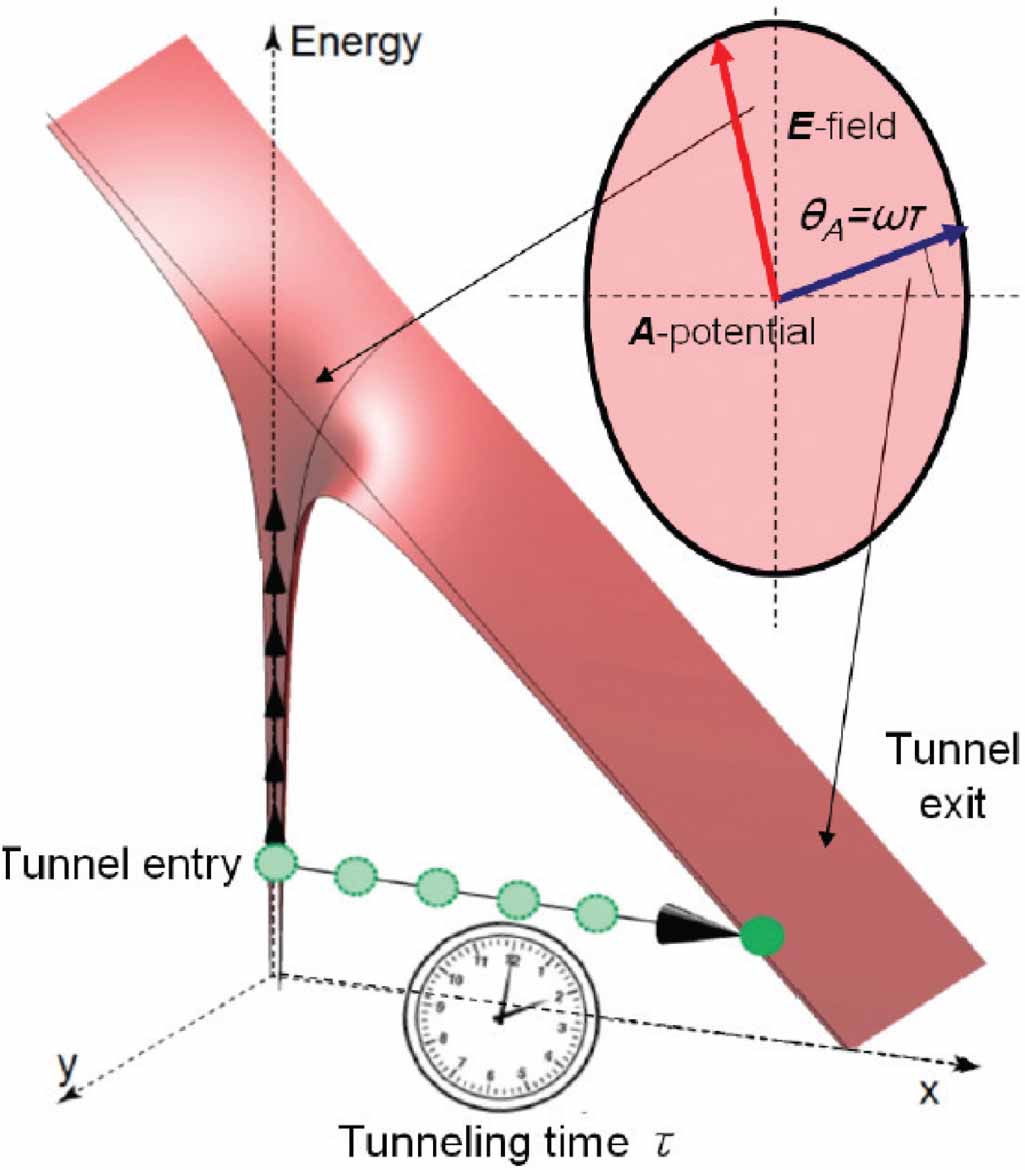
The attoclock is a self-referencing technique in which both the tunneling ionization and the subsequent steering of the photoelectron is driven by the same strong, close-to-circular IR pulse (Eckle et al 2008, Pfeiffer et al 2012). The principle of the attoclock is illustrated in figure 9. The Coulomb potential, which binds the atomic electron, is tilted by the strong electric field of the driving pulse. The bound electron is able to tunnel through the potential barrier. The tunneling starts when the electric field of the driving pulse is at its maximum. The photoelectron exits the tunnel with a cloe to zero velocity and its canonical momentum captures the vector potential of the driving field. This conserving momentum is carried to the detector where it becomes the kinetic momentum as the driving pulse is off at the arrival. The tilt angle of the photoelectron momentum at the detector relative to the vector potential at the start of tunneling (the minor polarization axis of the laser pulse) is converted to the tunneling time $\tau = \theta_A/\omega$.

Zoom In Zoom Out Reset image size

Unlike the Wigner time which is a thought quantity that can only be deduced from measuring the Wigner phase, it is claimed that the tunneling time is real and can be measured directly. This claim has been challenged both theoretically (Torlina et al 2015, Ni et al 2016, 2018, Bray et al 2018) and experimentally (Sainadh et al 2019) and the issue is under debate at present (Hofmann et al 2019, 2021, Kheifets 2020, Sainadh et al 2020).

In an attempt to reconcile the concepts of the Wigner time and the tunneling time, Yakaboylu et al (2014) performed quasi-classical trajectory simulations in a classically inaccessible region inside the tunnel. These simulations were used to interpret the experimental results by Camus et al (2018) in terms of a finite tunneling time. In section 2.2 we showed that the Wigner time delay can be visualized by the back propagation of the photoelectron trajectory to the origin and its termination at a 'time zero' that is displaced relative to the peak electric field of the driving laser pulse. This displacement is the measure of the Wigner time delay. In the attoclock, the tunnel exit extends to many Bohr radii away from the origin. Termination of the photoelectron trajectory at such a large distance results in a seemingly large 'Wigner' tunnelling time running in 100s of as. However, such a Wigner-like definition of the tunnelling time is questionable as a classical photoelectron trajectory cannot be continued into a classically inaccessible region under the barrier. Moreover, tunneling acts as an energy filter, favouring higher-energy components of the EWP and distorting the group delay (Hofmann et al 2019).

There had been several attempts to improve the original concept of the attoclock by adding a secondary field. Han et al (2019) superimposed a weak linearly polarized field to a long circularly polarized ionizing pulse. Because of an exponential sensitivity of the tunneling ionization, such a superposition produces a pronounced peak in the PMD which can be easily traced, both experimentally and numerically. In their Wigner function simulation, Han et al (2019) found quite a significant photoelectron exit time exceeding 200 as. However, this exit time appeared to be decoupled from the observed attoclock tilt angle which was wholly attributed to the Coulomb field of the ion reminder.

Closely related to an improved attoclock is the concept of holographic angular streaking of electrons (HASE) introduced by Eckart (2020). In HASE, two corotating circular pulses are used with the central frequencies 2ω (the driver, strong intensity) and ω (the stirrer, weak intensity). This field configuration gives rise to a subcycle interference pattern which is reflected in the PMD. This way HASE allows for the measurement of the phase of the initial wave packet in the momentum space at the tunnel exit.

3.3.1. Attoseond angular streaking of XUV ionization ASX.

This method was developed for a shot-to-shot characterization of isolated attosecond pulses at free-electron lasers (FEL) (Hartmann et al 2018, Duris et al 2020). Angular streaking of XUV ionization (ASXUVI or ASX for brevity) has common elements with the attosecond streak camera (section 3.1.4) and the attoclock (section 3.2). As in ASC, ASX uses XUV pulses to ionize the target. Then, similarly to the attoclock, the photoelectrons are steered by a circularly polarized laser field which makes its imprint on the photoelectron momentum distribution (PMD). This imprint is most graphical in the plane perpendicular to the laser propagation direction as illustrated in figure 10.

Zoom In Zoom Out Reset image size

The ASX as suggested initially (Kazansky et al 2016, 2019, Li et al 2018), employed an intense IR laser field and was interpreted within the strong field approximation (SFA) (Zhao et al 2022). In these strong field settings, the phase of the XUV ionization is commonly neglected and the timing information associated with this phase is lost. Kheifets et al (2022) provided an alternative interpretation based on the interferometric streaking picture as illustrated in the right panel of figure 6. This way the streaking phase was reintroduced to ASX and thus could be extracted from the PMD. Such an extraction is illustrated in figure 11.

Zoom In Zoom Out Reset image size

In the left panel of this figure, we plot the up $k_+[0^\circ]$ and down $k_-[180^\circ]$ vertical displacements of the PMD lobes displayed in the right panel of figure 10. These displacements satisfies the following isochrone equation

$$\begin{align} k_\pm^2(\tau)/2-E_0 = \pm A_0\, k_\pm(\tau)\cos(\omega\tau+\Phi_S)\ . \end{align} \tag{ 29 }$$

In the SFA, the streaking phase $\Phi_S = 0$ (Kazansky et al 2016). As the streaking signal (29) oscillates with the ω frequency, the corresponding time delay can be expressed as $\tau_S = \Phi_S/\omega$. The RABBITT signal (24) oscillates with the 2ω frequency, hence $\tau_R = \Phi_R/(2\omega)$. The corresponding time delays τ_S and τ_R in hydrogen are plotted in the right panel of figure 11 for various photoelectron energies. In the same plot we display the RABBITT data for the Yukawa atom in which the Coulomb field of the nucleus is fully screened while the ionization potential of the hydrogen atom is maintained. We observe from this figure that $\tau_S \approx\tau_R$ for the hydrogen atom which validates the phase extraction method in ASX. Both determinations of the time delay agree well with analytic predictions for hydrogen (Pazourek et al 2013, Serov et al 2015). In the meantime, $\tau_R\approx0$ for the Yukawa atom. This illustrates the Coulomb origin of the Wigner time delay and the CC correction in hydrogen.

3.3.2. High-order harmonics generation HHG.

The high-order harmonics generation (HHG) process makes an up frequency conversion of the IR driving pulse to the XUV spectral range. The simpleman three-step model (Corkum 1993) describes this process as (i) tunnel ionization of the traget atom, (ii) driven acceleration of the photoelectron by the laser field and its return to the origin and (iii) recombination of the photoelectron with the parent ion. As recombination is the time reversal of photoemission, the ionization phase and hence the Wigner time delay are encoded in it. It was believed that the spectral phase of HHG is shaped mostly by the photoelectron interaction with the driving IR field. However, it was demonstrated both experimentally (Schoun et al 2014) and theoretically (Brown et al 2022) that the recombination phase makes a significant contribution to the HHG spectrum and can be truthfully retrieved from it. An important specificity of HHG compared to photoionization is the selection of particular angular components of the target orbital and the photoelectron momenutm (Higuet et al 2011). First, tunnel ionization selects the quantization axis of the atomic orbital parallel to the polarization axis of the IR generating field. Then the IR field drives the trajectory of the recombining electron along the same axis.

Schoun et al (2014) used a RABBITT measurement in which the spectral harmonic phase (the attochirp) is usually considered as an unwanted instrumental effect. This effect is typically eliminated in comparative measurements (see section 3.1.1). Schoun et al (2014) turned this effect to a practical use and was able to measure the recombination phase near the CM of the 3 p shell of Ar. This phase can be expressed as the argument of the recombination amplitude

$$\begin{align*} D_{\boldsymbol{k}\to 3p}= {1\over\sqrt3} \left[ R_{Es\to 3p}e^{i\delta_0} - 2R_{Ed\to 3p}e^{i\delta_2} \right]. \end{align*}$$

Here the exponential terms contain the photoelectron scattering phases $\delta_\ell$ and $R_{E\ell\to 3p}$ are the corresponding radial integrals. Results of Schoun et al (2014) are shown in figure 12. Here the TDSE simulation reproduces the experiment accurately whereas the RPAE calculation misses some of the phase variation above the CM.

Zoom In Zoom Out Reset image size

As was highlihted in section 2.1, the phase of the EWP (9) contains the sum of several partial waves supported by corresponding spherical harmonics. Hence the Wigner time delay could be angular dependent. The first experimental observation of the angular dependent time delay was made by Heuser et al (2016) who measured this effect in helium using the RABBITT technique. The authors noted that the single XUV photon absorption by the He 1 s orbital leads to the sole p partial wave and the Wigner time delay in such a case should not depend on the photoelectron emission angle. The observed angular dependence was attributed to the auxiliary IR photon absorption that lead to the two competing s and d partial waves in the final photoelectron continuum. This effect was encoded in the angular dependent CC correction.

The true angular dependence of the Wigner time delay can be observed in heavier noble gases. Here the valence np shell ionization leads to the competing s and d partial waves and the Wigner time delay becomes angular dependent. This effect was predicted theoretically in Ne (Ivanov and Kheifets 2017) and heavier noble gases (Bray et al 2018a , 2018b ). An illustration of this effect is presented in figure 13.

Zoom In Zoom Out Reset image size

Experimentally, the angular dependent time delay was measured in RABBITT on Ar (Cirelli et al 2018, Busto et al 2019) and Ne (Joseph et al 2020). Cirelli et al (2018) observed anisotropic photoemission time delays close to the Fano $3s^{-1}4p$ resonance in Ar. Their results showed that the atomic time delay measured near the resonance depends strongly on the electron emission angle relative to the polarization of the ionizing XUV field. The ratio of the ionization channels $3p\to Ed$ and $3p\to Es$ abruptly changes across the resonances, leading to a strong variation of the ionization delay with the electron emission angle and energy.

A conventional RABBITT measurement does not allow to disentangle the competing photoemission channels and to resolve their individual spectral phases. In a polarization-skewed and angular dependent RABBITT scheme introduced by Jiang et al (2022) such a determination can be made for each partial wave. In this scheme, polarization axes of the XUV and IR laser pulses are rotated from a parallel to a perpendicular orientation. This way the contribution of different partial waves is manipulated.

Relativistic theory outlined in section 2.4 predicts a significant variation of the photoelectron phase and the Wigner time delay between various SO split ionization channels. Particularly strong such a variation is expected in the inner shells of heavy atoms. Banerjee et al (2020) predicted a very considerable SO effect on the time delay near the threshold of the 3d ionization of xenon. Similar effects can still be observed in valence shells of heavy atoms. By using RABBITT, Jordan et al (2017) and Jain et al (2018b) measured time delay from the SO split valance orbitals $4p_{\frac12/\frac32}$ in Kr and $5p_{\frac12/\frac32}$ in Xe. In the subsequent RABBITT measurements, Jain et al (2018a) and Zhong et al (2020) reached the inner $4d_{\frac32/\frac52}$ shell of Xe.

In lighter atoms, the relativistic effects in the photoemission phase and the Wigner time delay are notable close to sharp spectral features such as Fano resonances (Turconi et al 2020) and Cooper minima (Saha et al 2014, Ganesan et al 2020, Kheifets et al 2020). Turconi et al (2020) measured the spectral phase across the $3s^{-1}4p$ Fano resonance in argon for both the SO components by using RABBIT with a very fine energy resolution. Such a measurement allowed for a complete separation of the two SO components.

A notable manifestation of relativistic effects can be seen in an angular dependent time delay near correlation induced Cooper minima in noble gas atoms. Such CM can be seen in photoionization cross-sections of valence shells of Ar, Kr and Xe. The corresponding photoionization amplitudes change their sign and the phase makes a jump close to π as can be seen in figure 10 for the 3 p shell of Ar. As was noted in section 4.1, a non-relativistic time delay in an ns atomic shell is angular independent because of a single photoionization channel ns → Ep. The SO interaction splits the continuum into the two channels $ns\to Ep_{\frac12/\frac32}$ each of which passes through its respective CM at a slightly different photoelectron energy. As a result, the photoemission phase and the Wigner time delay become angular dependent. This effect is displayed in figure 14 near the 3 s CM in argon.

Zoom In Zoom Out Reset image size

Up to now, we considered ionization processes involving emission of a single photoelectron and leaving the remaining ion in its ground state. However, if a sufficient energy is transferred to the target atom, two or more electrons can be ejected. Alternatively, this energy may be used to promote one or several of the target electrons to excited states when the photoelectron leaves the atom. In this section we restrict ourselves with two-electron ionization processes such as double photoionization (DPI) and single ionization with excitation (shake up—SU). Both processes are driven by a single XUV photon absorption and involve simultaneous (non-sequential) two-electron transition. Such a transition can only be facilitated by many-electron correlation. So the time resolution of DPI and shake-up processes allows to gauge this correlation on the time scale. Several theoretical investigations of time-resolved DPI (Kheifets et al 2011, Kheifets and Bray 2021b, Kheifets 2022a) and shake up (Pazourek et al 2012, Donsa et al 2020) have been reported to date.

The time resolved RABBITT measurement of DPI was conducted by Mansson et al (2014) in the Xe atom. They clocked the DPI against the single photoionization and observed a considerable time lag between the two processes. The experimental time resolution of the shake-up ionization channel was achieved by Isinger et al (2017) who disentangled the ground state ionization of the 2s shell in Ne with an accompanying $2p^{-2}nl$ SU satellite. While the time delay difference between the $2s^{-1}$ and $2p^{-1}$ ionic states was found in excellent agreement with theory, the time delay between the SU and $2p^{-1}$ appeared to be consistently larger in magnitude. Isinger et al (2017) noted that the influence of shake-up processes on the earlier streaking experiment by Schultze et al (2010) was investigated theoretically in Dahlström et al (2012) and not found to explain the difference between theory and experiment. Similar conclusion was reached by Nicolaides (2018). Consistently large SU-2p time delay, of the order of 50 as, across a wide photoelectron energy range of 10 eV, means a spectral phase variation of about 0.8 radians. No such phase variation can be found in any of the Ne ionization continua in the photoelectron energy range of interest (see figure 3 left). The correlation induced phase in the SU process in Ne is also small (Kheifets 2022a). In the meantime, RABBITT instrumental effects could be responsible for seemingly large SU time delay as was found to be the case in the argon measurement by Alexandridi et al (2021).

A complicated potential landscape of molecules is capable to produce a significant variation of the Wigner time delay both with the photoelectron energy and its emission angle. The energy variation can be particularly strong near sharp spectral features such as shape resonances. In addition, molecular vibration can be an additional factor affecting the Wigner time delay. All these effects stimulate a strong interest in time-resolved photoionization studies on molecular targets.

The first theoretical prediction of an angular asymmetry of the Wigner time delay in a small hetero-nuclear molecule was made by Chacon et al (2014). An effect of the two-center interferences on the attosecond streaking of the H$_2^+$ molecular ion was studied theoretically (Ning et al 2014, Serov and Kheifets 2016). A broad theoretical study of time delays in molecular photoionization was conducted by Hockett et al (2016).

The spectral phase of molecular ionization was first determined experimentally by Haessler et al (2009) and then analysed theoretically by Caillat et al (2011). The first experimental study of the Wigner time delay in molecules was reported by Huppert et al (2016) in their RABBITT measurements on N₂O and H₂O. These results were interpreted theoretically by Baykusheva and Wörner (2017) and Serov and Kheifets (2017). Stimulated by theoretical predictions of an anisotropic time delay in hetero-nuclear molecules, Vos et al (2018) conducted RABBITT measurements on CO and introduced a concept of the stereo Wigner time delay. It was confirmed that it would indeed take a considerably different time to detect a photoelectron emitted from the carbon and oxygen ends. RABBITT allowed to measure the photoelectron group delay in the shape resonance region of various molecules: N₂ (Haessler et al 2009, Nandi et al 2020, Loriot et al 2021), N₂O (Huppert et al 2016), CO₂ (Kamalov et al 2020), NO (Gong et al 2022) and CF₄ (Heck et al 2021, Ahmadi et al 2022). A similar shape resonance measurement in NO (Driver et al 2020) was conducted using the ASX technique (Kheifets et al 2022). Probing molecular environment through photoemission delays in the complex CH₃I molecule was conducted by Biswas et al (2020).

A novel technique of photoelectron phase determination and their conversion to the Wigner time delay was implemented by Rist et al (2021) and Holzmeier et al (2021). This technique is related to the concept of a complete photoemission experiment in which the photoelectron angular distribution (PAD) is determined by a set of dipole matrix elements and phase differences (Cherepkov et al 2000). By fitting the experimental PAD with such a set, both groups of authors were able to trace the photoelectron phases across a range of energies and to convert them to the corresponding Wigner time delays. Trabert et al (2021) used the HASE technique to measure the angular dependent Wigner time delay in H₂.

A clear indication of the coupled electron-nuclear attosecond dynamics was presented in the RABBITT measurement on H₂ by Cattaneo et al (2018, 2022). This effect was investigated in more detail by Wang et al (2021) who studied the role of nuclear-electronic coupling in attosecond photoionization of H₂. Theoretically, this effect was studied by Kowalewski et al (2016) using nuclear autocorrelation functions.