
Abstract
Aims: tungsten has been chosen for use as a plasma facing component in the divertor for the ITER experiment, and is currently being used on existing tokamaks such as JET. W+ plays an integral role in assessing the impurity influx from plasma facing component of tokamaks and subsequent redeposition. Together with previously calculated a neutral tungsten electron-impact dataset this study allows us to determine neighbouring spectral lines in the same wavelength window of the spectrometer, and detect if there is strong blending of overlapping lines between these two ion stages as well as providing ionisation per photon ratios for both species. The new data is to be used for tungsten erosion/redeposition diagnostics. Methods: a significantly modified version of the GRASP0 atomic structure code in conjunction with DARC (Dirac Atomic R-matrix Code) are used to calculate the Einstein A coefficients and collisional rates used to generate a synthetic W II spectrum. The W II spectrum is compared against tungsten spectral emission experiments. Results: this study is used to model the spectrum of W ii, providing the predictive capability of identifying spectral lines from recent experiments. These results provide an integral part of impurity influx and redeposition determination, as the ionisation rates may be used to calculate S/XB ratios.
Export citation and abstract BibTeX RIS

Original content from this work may be used under the terms of the Creative Commons Attribution 4.0 licence. Any further distribution of this work must maintain attribution to the author(s) and the title of the work, journal citation and DOI.
1. Introduction
Tungsten is being employed as a plasma facing component (PFC) in the divertor region of ITER [1] and other ongoing tokamak experiments [2, 3]. The impurity influx of tungsten from PFCs into the plasma is undesirable, as highlighted by P tterich et al [4], yet its quantification remains important if we are to determine tungsten erosion and redeposition. Earlier work of Isler [5] and Murakami et al [6] states that the presence of as little as 0.1% of this high-Z element, within the plasma may be sufficient to quench the reaction, confirmed by P
 tterich et al [4] but at even smaller quantities. The impurity influx is a critical issue for fusion reactor design, and is one of the primary motivations for this study. The atomic structure combined with electron-impact excitation and effective ionisation rates underpin reliable erosion diagnostics to characterise the influx of tungsten impurities into the core plasma. In recent years there has been much focus on the calculation of relevant data for highly charged tungsten species. Examples of such works include; Turkington et al [7] (W63+), Hussein et al [8] (W39+), El-Maaref et al [9] (W44+) and Aggarwal [10] (W44+). Less focus has been placed on data for the low-ion stages of tungsten. While the work of Smyth et al [11] presents extensive calculations for neutral tungsten there is a very noticeable gap in available collisional data for its neighbouring ion stages, specifically W+ and W2+. Calculations for W3+ have been presented previously in the work of Ballance et al [12].
The ITER tokamak is currently under construction in Cadarache, France, and must address these problems of impurity influx and plasma stability. Benchmarking new atomic data for the low charge states of W is a challenge. The Compact Toroidal Hybrid (CTH) experiment at Auburn University can measure W spectra to assist benchmarking photon emissivities, and thus indirectly benchmark the electron-impact excitation rate coefficients and spontaneous emission coefficients. Due to the ongoing importance of tungsten to ITER, it was also crucial to provide atomic data for neutral system. Therefore, Smyth et al [11] calculated the electron-impact excitation cross sections for fine structure transitions in W I. These atomic data are integrated into the collisional-radiative modelling codes [13] to aid in the development of diagnostic for gross erosion rates [14]. Theoretically, it is electron-impact excitation/ionisation calculations that are needed for such erosion diagnostics.
Historically, the modelling of singly ionised tungsten has only slowly progressed to sufficient accuracy required to complete such a thorough analysis. The first experimental study of this ion stage was completed by Laun [15], and presented 77 energy levels that were derived from 500 W II lines which ranged in wavelength from 1961.43 Å to 4348.13 Å. Laun continued working on analysing W II and published a second paper [16], comprising of 194 levels from 4 configurations, which included, 5d46p, 5d46s, 5d36s6p, and 5d26s26p. 2173 transitions were observed from 1756.6 Å to 6219.77 Å. Further wavelengths for W II were published by Cabeza et al [17], with the experiment carried out by forming a low-voltage sliding spark discharge which was recorded photographically on the National Institute of Science and Technology (NIST) 10.7 m normal incidence vacuum spectrograph [18] in the 600–2680 Å spectral region. Theoretically, low even parity configurations were analysed through the use of a parametric method by Wyart [19] using energy levels supplied by Laun [16], where nine experimental levels were omitted in the least square fit.
Continuing his work, and in collaboration with Blasé, Wyart repeated a similar calculation for the low-lying odd parity configurations, such as, 5d46p, 5d36s6p and 5d26s26p. 132 experimental levels were identified by Wyart and Blasé [20]. However, these calculations were limited with respect to the small number of configurations considered. An experimental study carried out by Ekberg et al [21] identified almost 2500 spectral lines in the region of 1850 Å to 5800 Å, analysed using a Penning discharge spectrogram obtained with a Fourier transform spectrograph. Wavelengths were also identified from a similar set of configurations but employing the HFR code of Cowan [22]. Even (5d5, 5d46s and 5d36s2) and odd configurations (5d46p, 5d36s6p and 5d26s26p) were included in the calculations. Further spectral lines were presented in the work of Kling et al [23] for the same spectral region. More recently, Kramida and Shirai [24] presented energy levels, wavelengths, and transition probabilities for W ii. Quinet et al [25] presented transition probabilities for allowed and forbidden lines in neutral, singly ionised and doubly ionised tungsten. They summarised the existing electric dipole transitions identified from the literature, and obtained both magnetic dipole and electric quadrupole transitions using the relativistic Hartree–Fock method.
Lennartsson et al [26] recorded spectra of W ii between 1950–4350 Å, observed using a spectrometer (FT500 UV Fourier Transform Spectrometer). These observations were incorporated with previous data measured by the time resolved laser induced fluorescence technique, resulting in transition probabilities and log gf values for W ii. They observed 95 transitions which originated from 9 upper levels. Only 15 of these transitions had been measured previously. Since Lennartsson et al [26] completed their study, there has been a conference paper by Husain et al [27] where they carried out calculations using the cowan code [22], and the levels used to complete the least square fit were taken from National Institute of Standards and Technology (NIST [28]).
Despite the efforts of these investigations into W ii there exists no comprehensive and publicly available close-coupled datasets for electron-impact excitation, preventing the determination of erosion diagnostics for fusion plasmas. We have carried out an evaluation of the electron-impact excitation for W ii. These atomic data can then be integrated into sophisticated modelling codes to provide impurity influx predictions. We compare with the transition probabilities in NIST, which contain data provided by Ekberg et al [21], Lennartsson et al [26] and Quinet et al [25]. After completing the electron-impact excitation calculations for W ii, we have carried out collisional-radiative modelling in order to generate a synthetic spectra from our data. The data set is compared to spectra observed from recent CTH measurements.
In the present work we compare with Johnston et al [14], who carried out an analysis of the spectral lines of tungsten. Their recent observations found unidentified lines in the spectrum produced by the CTH experiment, suspected to be W II. Having two ion stages emitting within the same wavelength window of the spectrometer, provides greater confidence in any temperature or density determinations. To achieve a complete picture of the spectra it is highly desirable to provide further diagnostics at densities and temperatures relevant to the conditions expected in ITER. We have difficulty identifying lines due to the fact that NIST [28] does not provide a complete dataset for comparison. Therefore, CTH experiments, cowan code calculations and grasp calculations may aid in the designations of lines.
In section 2 we investigate the atomic structure using the multi-configurational Dirac–Fock method, implemented by grasp0 [29]. We present three calculations, the first an 8 configuration model to provide a benchmark for comparison with the second model, a 13 configuration model. A third calculation presents an extensive 17 configuration model. In section 3 we discuss our electron-impact excitation calculations using the R-matrix codes (DARC) [30]. Lastly, in section 4 we present our population modelling calculations, benchmarked against recent CTH measurements.
2. GRASP0: atomic structure
W+ has a complex atomic structure due to the open d shell nature of both the ground and excited states. Our goal is to describe the spectrum of W+ at temperatures and densities pertinent to the interpretation of spectra from magnetically-confined plasmas. Difficulties may arise when comparing the present theoretical calculations with existing work due to the strong mixing of excited state levels and the lack of identified and labelled observed data (see figure 1). Three calculations were completed, based upon three different configuration lists and the resulting energy levels calculated using the relativistic grasp0 (General Purpose Relativistic Atomic Structure Package, [29]). grasp0 which implements the multi-configuration Dirac Hartree Fock method, solving the time independent Dirac equation (TIDE),

where ϕ is the Dirac orbital, and E corresponds to energy eigenvalues of the Hamiltonian. Specifically the Dirac–Coulomb Hamiltonian HD can be defined as,

where c is the speed of light, and p is the momentum operator defined as p = −iℏ∇. The parameters α and β are Dirac matrices.

Figure 1. Energy level spectrum of W ii organised by electronic configuration (for the first 5 configurations which contribute to the lowest-lying levels). Each horizontal line designates a specific fine structure level (taken from the NIST database).
Download figure:
Standard image High-resolution imageWith grasp0 we used the extended average level (EAL) method. For the EAL method we optimise the Hamiltonian on the weighted sum of the diagonal matrix elements,

where rij = |rj − ri |. Initially, we construct a relatively small model in order to create a benchmark for our more complex structure described later. This model contained 16 orbitals, and 8 non-relativistic configurations, described below,
| 4f145s25p65d46s | 4f145s25p65d46d | 4f145s25p65d36s2 |
| 4f145s25p45d7 | 4f145s25p65d46p | 4f145s25p65d36s6p |
| 4f145s25p65d5 | 4f145p65d7, |
| 4f145s25p65d5 | 4f145s25p65d36s2 | 4f145s25p65d36s6d |
| 4f145s25p65d46s | 4f145s25p55d56d | 4f145s25p65d36s6p |
| 4f145s25p65d46p | 4f145s25p55d56p | 4f145s25p65d36p2 |
| 4f145s25p65d46d | 4f145s25p55d56s | 4f145s25p65d36d2 |
| 4f145s25p45d7. |
resulting in 1068 jj-levels. The energy levels produced from this model did show promising results, particularly for the odd parity states. This model will be known as model 1 for the duration of this paper.
Even though model 1 showed promising results, the low-lying even parity states had an average percentage error of around 20%, in terms of absolute energy relative to the ground state, when compared with the existing literature. This necessitated a second more sophisticated model.
In the second model we created a more complex structure, containing all the configurations from the first model but also allowing all single and double promotions from the 5d orbital to the 6d orbital, and double promotion to the 6p orbital were also included. In order to build up the structure for the second model the 6p and 6d orbitals were introduced separately. This was a larger model containing 13 non-relativistic configurations,
This resulted in a 5816 jj-level structure, and shall be referred to as model 2 throughout the rest of the paper. This model showed very promising results. However, comparisons with the CTH experiment showed additional spectral lines (dipole transitions) not included in this model. Therefore, we created a third model containing 17 non-relativistic configurations. The building up of the configurations for this model is presented in table 1. The initial model included 11 configurations, giving rise to 6910 close coupled channels, which was reduced to 2626 channels by removing configurations which caused a lot of configuration interaction but did not contribute value to the model. Configurations were also included that contained the 7s orbital. Finally further configurations were incorporated, including configurations containing the 7p orbital. The corresponding energy levels can be found in table 2. This final model contains,
| 4f145s25p65d5 | 4f145s25p65d36s2 | 4f145s25p45d46s7s2 |
| 4f145s25p65d46s | 4f145s25p65d36p2 | 4f145s25p65d36s6p |
| 4f145s25p65d46p | 4f145s25p65d36d2 | 4f145s25p45d66s |
| 4f145s25p65d46d | 4f145s25p65d37s2 | 4f145s25p55d56s |
| 4f145s25p55d57s | 4f145s25p65d37p2 | 4f145s25p45d7 |
| 4f145s25p65d47p | 4f145s25p45d56s2. |
Table 1. Table showing the development of the configuration set for the grasp0 atomic structure of model 3 for singly ionised tungsten.
| Model | No. of levels | Configurations included |
|---|---|---|
| M3a | 6910 | 5s25p65d5 |
| 5s25p65d4 {6s,6p,6d}, | ||
| 5s25p65d3 {6s2,6p2,6d2}, | ||
| 5s25p4 {5d66s,5d66d,5d7}, | ||
| 5s25p55d56s | ||
| M3b | 2626 | M3a + 5s25p65d37s2,5s25p55d57s − 5s25p4 {5d66s,5d66d} |
| M3 | 5509 | M3b + 5s25p6 {5d36s6p,5d47p,5d37p2}, 5s25p4 {5d66s,5d46s7s2,5d56s2} |
Table 2. A representative sample of fine structure energies of W ii, in Ryds (relative to the ground state). Energies from the various grasp0 models are presented and are compared to the experimental values (Expt) compiled by Kramida and Shirai [24].
| No. | Config. | Level | M3a | M3b | M3 | Expt |
|---|---|---|---|---|---|---|
| 1 | 5d46s | 6D1/2 | 0.000 00 | 0.000 00 | 0.000 00 | 0.000 00 |
| 2 | 5d46s | 6D3/2 | 0.134 17 | 0.008 19 | 0.008 98 | 0.013 84 |
| 3 | 5d46s | 6D5/2 | 0.149 08 | 0.019 20 | 0.020 68 | 0.028 91 |
| 4 | 5d46s | 6D7/2 | 0.167 29 | 0.031 54 | 0.033 47 | 0.042 98 |
| 5 | 5d46s | 6D9/2 | 0.177 00 | 0.044 70 | 0.046 86 | 0.056 02 |
| 6 | 5d5 | 6S5/2 | 0.185 62 | 0.085 21 | 0.065 79 | 0.067 62 |
| 7 | 5d36s2 | 4F3/2 | 0.187 05 | 0.097 22 | 0.076 57 | 0.079 38 |
| 8 | 5d46s | 4P1/2 | 0.193 68 | 0.099 68 | 0.092 28 | 0.080 49 |
| 9 | 5d36s2 | 4P3/2 | 0.198 37 | 0.106 32 | 0.105 05 | 0.096 53 |
| 10 | 5d36s2 | 4F5/2 | 0.203 38 | 0.112 62 | 0.099 21 | 0.102 98 |
| 11 | 5d46s | 4D1/2 | 0.203 74 | 0.127 36 | 0.126 09 | 0.120 04 |
| 12 | 5d36s2 | 4F7/2 | 0.212 37 | 0.139 48 | 0.121 66 | 0.122 22 |
| 13 | 5d36s2 | 4P5/2 | 0.212 85 | 0.140 56 | 0.131 08 | 0.122 42 |
| 14 | 5d46s | 4D3/2 | 0.228 88 | 0.145 80 | 0.138 63 | 0.133 36 |
| 15 | 5d36s2 | 4F9/2 | 0.230 97 | 0.151 89 | 0.141 59 | 0.135 39 |
| 16 | 5d46s | 4D5/2 | 0.236 75 | 0.163 36 | 0.150 67 | 0.136 40 |
| 17 | 5d46s | 4H7/2 | 0.239 29 | 0.166 32 | 0.173 74 | 0.138 03 |
| 18 | 5d46s | 4G5/2 | 0.285 37 | 0.173 78 | 0.178 79 | 0.147 94 |
| 19 | 5d46s | 4H9/2 | 0.286 38 | 0.178 50 | 0.177 48 | 0.150 84 |
| 20 | 5d46s | 4D5/2 | 0.307 26 | 0.186 93 | 0.161 08 | 0.151 18 |
| 21 | 5d46p |
6

| 0.569 30 | 0.328 12 | 0.340 02 | 0.329 56 |
| 22 | 5d36s6p |
6

| — | — | 0.352 01 | 0.346 02 |
| 23 | 5d46p |
4

| 0.591 74 | 0.527 08 | 0.353 16 | 0.351 53 |
| 24 | 5d46p |
6

| 0.587 29 | 0.338 12 | 0.355 69 | 0.356 57 |
| 25 | 5d36s6p |
6

| — | — | 0.367 37 | 0.363 93 |
| 26 | 5d46p |
6

| 0.609 11 | 0.352 30 | 0.750 00 | 0.383 18 |
| 27 | 5d46p |
6

| 0.655 04 | 0.353 12 | 0.378 57 | 0.385 45 |
| 28 | 5d36s6p |
6

| — | — | 0.385 85 | 0.386 29 |
| 29 | 5d46p |
6

| 0.692 23 | 0.395 21 | 0.398 01 | 0.404 19 |
| 30 | 5d36s6p |
6

| — | — | 0.405 93 | 0.405 11 |
| 31 | 5d46p |
6

| 0.660 56 | 0.390 82 | 0.405 93 | 0.407 87 |
| 32 | 5d46p |
6

| 0.633 40 | 0.369 74 | 0.390 52 | 0.408 95 |
| 33 | 5d46p |
6

| 0.626 58 | 0.404 00 | 0.402 13 | 0.409 27 |
| 34 | 5d46p |
6

| 0.704 78 | 0.424 21 | 0.394 84 | 0.414 24 |
| 35 | 5d36s6p |
6

| — | — | 0.410 24 | 0.415 12 |
| 36 | 5d36s6p |
6

| — | — | 0.413 21 | 0.420 78 |
| 37 | 5d36s6p |
6

| — | — | 0.422 24 | 0.423 68 |
| 38 | 5d36s6p |
6

| — | — | 0.434 30 | 0.424 88 |
| 39 | 5d36s6p |
6

| — | — | 0.447 70 | 0.429 94 |
| 40 | 5d46p |
6

| 0.692 23 | 0.413 96 | 0.452 25 | 0.432 06 |
This resulted in a 5509 jj-level structure. We will refer to this model as model 3 for the remainder of this paper.
2.1. Atomic structure evaluation
It is necessary to evaluate the accuracy of our models. For atomic structure evaluations, a well established method of testing accuracy is to compare the energy levels and oscillator strengths with existing observed and theoretical data in the literature, such as the values found in NIST [28].
Table 3 displays the energy levels in Ryds for 24 energy levels (the first 20 lowest lying even parity states, and 4 lowest lying odd parity states) of W+ included in both model 1, model 2 and model 3. These energy levels are evaluated against energy levels compiled by Kramida and Shirai [24] (recorded on NIST).
Table 3. Comparing energy levels of all presented models with NIST values (this is the work of Kramida and Shirai [24]). All energy values are listed in Rydbergs.
| No. | Configuration | J | Parity | Model 1 (Ryd) | Model 2 (Ryd) | Model 3 (Ryd) | NIST (Ryd) | Absolute error 1 | Absolute error 2 | Absolute error 3 |
|---|---|---|---|---|---|---|---|---|---|---|
| 1 | 5p65d46s (6D) | 1/2 | Even | 0.000 × 101 | 0.000 × 101 | 0.000 × 101 | 0.000 × 101 | 0.00 × 101 | 0.00 × 101 | 0.00 × 101 |
| 2 | 5p65d46s (6D) | 3/2 | Even | 5.672 × 10⁻³ | 8.749 × 10⁻³ | 8.984 × 10⁻³ | 1.384 × 10⁻² | 4.07 × 10⁻³ | 5.09 × 10⁻³ | 4.86 × 10⁻³ |
| 3 | 5p65d46s (6D) | 5/2 | Even | 1.921 × 10⁻² | 2.023 × 10⁻² | 2.068 × 10⁻² | 2.891 × 10⁻² | 9.69 × 10⁻³ | 8.68 × 10⁻³ | 8.23 × 10⁻³ |
| 4 | 5p65d46s (6D) | 7/2 | Even | 3.173 × 10⁻² | 3.287 × 10⁻² | 3.347 × 10⁻² | 4.298 × 10⁻² | 1.12 × 10⁻² | 1.01 × 10⁻² | 9.51 × 10⁻³ |
| 5 | 5p65d46s (6D) | 9/2 | Even | 4.514 × 10⁻² | 4.621 × 10⁻² | 4.686 × 10⁻² | 5.602 × 10⁻² | 1.09 × 10⁻² | 9.81 × 10⁻³ | 9.16 × 10⁻³ |
| 6 | 5s25p65d5 (6S) | 5/2 | Even | 6.062 × 10⁻² | 7.116 × 10⁻² | 6.579 × 10⁻² | 6.762 × 10⁻² | 7.00 × 10⁻² | 3.54 × 10⁻³ | 1.83 × 10⁻³ |
| 7 | 5p65d36s2 (4F) | 3/2 | Even | 1.041 × 10⁻¹ | 9.123 × 10⁻² | 7.657 × 10⁻² | 7.938 × 10⁻² | 2.36 × 10⁻² | 1.18 × 10⁻² | 2.82 × 10⁻³ |
| 8 | 5p65d46s (4P) | 1/2 | Even | 1.060 × 10⁻¹ | 9.776 × 10⁻² | 9.228 × 10⁻² | 8.049 × 10⁻² | 2.66 × 10⁻² | 1.72 × 10⁻² | 1.18 × 10⁻² |
| 9 | 5p65d46s (4P) | 3/2 | Even | 1.171 × 10⁻¹ | 1.109 × 10⁻¹ | 1.050 × 10⁻¹ | 9.653 × 10⁻² | 2.06 × 10⁻² | 1.44 × 10⁻² | 8.52 × 10⁻³ |
| 10 | 5p65d36s2 (4F) | 5/2 | Even | 1.249 × 10⁻¹ | 1.113 × 10⁻¹ | 9.921 × 10⁻² | 1.030 × 10⁻¹ | 2.19 × 10⁻² | 8.29 × 10⁻³ | 3.77 × 10⁻³ |
| 11 | 5p65d46s (4D) | 1/2 | Even | 1.424 × 10⁻¹ | 1.366 × 10⁻¹ | 1.261 × 10⁻¹ | 1.200 × 10⁻¹ | 1.66 × 10⁻² | 1.66 × 10⁻² | 6.05 × 10⁻³ |
| 12 | 5p65d36s2 (4F) | 7/2 | Even | 1.439 × 10⁻¹ | 1.314 × 10⁻¹ | 1.217 × 10⁻¹ | 1.222 × 10⁻¹ | 2.17 × 10⁻² | 9.15 × 10⁻³ | 5.55 × 10⁻⁴ |
| 13 | 5p65d36s2 (4F) | 5/2 | Even | 1.390 × 10⁻¹ | 1.357 × 10⁻¹ | 1.311 × 10⁻¹ | 1.224 × 10⁻¹ | 2.48 × 10⁻² | 1.33 × 10⁻² | 8.66 × 10⁻³ |
| 14 | 5p65d46s (4D) | 3/2 | Even | 1.533 × 10⁻¹ | 1.484 × 10⁻¹ | 1.386 × 10⁻¹ | 1.333 × 10⁻¹ | 2.23 × 10⁻² | 1.50 × 10⁻² | 5.27 × 10⁻³ |
| 15 | 5p65d46s (4F) | 9/2 | Even | 1.602 × 10⁻¹ | 1.489 × 10⁻¹ | 1.416 × 10⁻¹ | 1.354 × 10⁻¹ | 1.99 × 10⁻² | 1.35 × 10⁻² | 6.20 × 10⁻³ |
| 16 | 5p65d46s (4D) | 5/2 | Even | 1.637 × 10⁻¹ | 1.590 × 10⁻¹ | 1.507 × 10⁻¹ | 1.364 × 10⁻¹ | 2.73 × 10⁻² | 2.26 × 10⁻² | 1.43 × 10⁻² |
| 17 | 5p65d46s (4H) | 7/2 | Even | 1.720 × 10⁻¹ | 1.642 × 10⁻¹ | 1.737 × 10⁻¹ | 1.380 × 10⁻¹ | 3.40 × 10⁻² | 2.62 × 10⁻² | 3.57 × 10⁻² |
| 18 | 5p65d46s (4G) | 5/2 | Even | 1.763 × 10⁻¹ | 1.724 × 10⁻¹ | 1.788 × 10⁻¹ | 1.480 × 10⁻¹ | 2.82 × 10⁻² | 2.44 × 10⁻² | 3.08 × 10⁻² |
| 19 | 5p65d46s (2H) | 9/2 | Even | 1.790 × 10⁻¹ | 1.730 × 10⁻¹ | 1.775 × 10⁻¹ | 1.508 × 10⁻¹ | 2.82 × 10⁻² | 2.22 × 10⁻² | 2.66 × 10⁻² |
| 20 | 5p65d46s (4D) | 7/2 | Even | 1.872 × 10⁻¹ | 1.766 × 10⁻¹ | 1.611 × 10⁻¹ | 1.512 × 10⁻¹ | 3.61 × 10⁻² | 2.53 × 10⁻² | 9.90 × 10⁻³ |
| 21 | 5p65d46p (6Fo) | 1/2 | Odd | 3.146 × 10⁻¹ | 3.177 × 10⁻¹ | 3.400 × 10⁻¹ | 3.296 × 10⁻¹ | 1.71 × 10⁻² | 1.19 × 10⁻² | 1.05 × 10⁻² |
| 22 | 5p65d36s6p (6Go) | 3/2 | Odd | 3.056 × 10⁻¹ | 3.042 × 10⁻¹ | 3.520 × 10⁻¹ | 3.460 × 10⁻¹ | 3.04 × 10⁻² | 4.18 × 10⁻² | 5.99 × 10⁻³ |
| 23 | 5p65d46p (4Po) | 1/2 | Odd | 3.293 × 10⁻¹ | 3.346 × 10⁻¹ | 3.532 × 10⁻¹ | 3.515 × 10⁻¹ | 2.23 × 10⁻² | 1.70 × 10⁻² | 1.63 × 10⁻³ |
| 24 | 5p65d46p (6Fo) | 3/2 | Odd | 3.297 × 10⁻¹ | 3.322 × 10⁻¹ | 3.557 × 10⁻¹ | 3.566 × 10⁻¹ | 2.69 × 10⁻² | 2.45 × 10⁻² | 8.81 × 10⁻⁴ |
For model 1 the atomic structure shows an average percentage error of 20.5% for the even parity levels, and 6.7% for the odd levels with the values of NIST. This indicates that model 1 provides an accurate representation for the configuration states containing a single promotion from the 5d orbital to the 6p (5p65d46p), and double promotions from the 5d orbital split between the 6s and 6p (5p65d36s6p). However, model 1 does not appear to be a sufficiently accurate representation for the configuration states containing single or double promotions from the 5d orbital to the 6s (5p65d46s and 5p65d36s2) as they exhibit much larger errors. As model 1 is comprised of only 8 configurations in the target wavefunction expansion, the model lacks configurations which when included may affect the configuration interaction expansion.
There is a significant improvement for model 2 as the atomic structure shows a reasonable average error of 7.7% for the even parity levels, ranging from 1.0% up to 17.2%. The odd parity levels are well represented having an average error of only 0.7%, with errors ranging from 0.002% up to 2.5%. These results indicates that model 2 provides an accurate representation for both the even and the odd configuration states. These uncertainties show continued improvement for model 3, the average error for the even parity levels decreases to 1.3% and the odd parity levels to 0.4%.
Another valid comparison metric is the transition probabilities. In table 4 the transition probabilities for both models have been compared with the values in NIST which have been obtained from the experiments of Ekberg et al [21] and Lennartsson et al [26]. For model 1 most of the values agree within the same order of magnitude, however there are values which are quite different from the measured values, such as for the 232.4285 nm wavelength with a value of 2.41 × 10⁴ s−1 which is 2 orders of magnitude smaller than the value of NIST (4.46 × 10⁶ s−1). This improves greatly for the second model which falls within the same order of magnitude as NIST. Model 3 improves to 5.98 × 10⁶ s−1. A similar trend can be seen in table 5 for the transitions when compared with the results from Quinet et al [25], the second model shows a more consistent agreement. The third model has better agreement across most of the forbidden lines. To compare the results of the improving atomic structure, calculations for the electron-impact excitation of W+ were carried out for all models.
Table 4. A-values (s−1) for dipole transitions for both models and the values available in NIST (Ekberg et al [21], Lennartsson et al [26]).
| Wavelength (nm) | Lower level | Upper level | A(s−1): | A(s−1): | A(s−1): | A(s−1): | A(s−1): |
|---|---|---|---|---|---|---|---|
| Level | Level | Ekberg et al (2000) | Lennartsson et al (2011) | Model 3 | Model 2 | Model 1 | |
| 232.4285 | 5s25p65d5 (6S5/2) | 5p65d46p (4
 ) ) | 4.46 × 10⁶ | 5.98 × 10⁶ | 1.72 × 10⁶ | 2.41 × 10⁴ | |
| 233.9733 | 5p65d36s2 (4F3/2) | 5p65d46p (4
 ) ) | 5.33 × 10⁶ | 8.54 × 10⁶ | 8.62 × 10⁶ | 1.79 × 10⁶ | |
| 234.9835 | 5p65d36s2 (4F3/2) | 5p65d36s6p (6
 ) ) | 7.14 × 10⁷ | 4.04 × 10⁷ | 5.92 × 10⁷ | 1.95 × 10⁷ | |
| 239.037 01 | 5s25p65d5 (6S5/2) | 5p65d36s6p (6
 ) ) | 6.69 × 10⁷ | 3.84 × 10⁷ | 4.86 × 10⁷ | 1.19 × 10⁸ | |
| 239.292 814 | 5p65d46s (6D7/2) | 5p65d36s6p (6
 ) ) | 2.28 × 10⁷ | 2.53 × 10⁷ | 2.22 × 10⁷ | 2.20 × 10⁷ | |
| 239.6219 | 5p65d36s2 (4F3/2) | 5p65d46p (4
 ) ) | 8.91 × 10⁶ | 6.44 × 10⁶ | 9.37 × 10⁶ | 2.94 × 10⁷ | |
| 239.707 936 | 5p65d46s (6D5/2) | 5p65d46p (6
 ) ) | 5.24 × 10⁷ | 5.69 × 10⁷ | 6.77 × 10⁷ | 1.13 × 10⁸ | |
| 240.3215 | 5p65d46s (4P1/2) | 5p65d46p (4
 ) ) | 3.42 × 10⁶ | 4.84 × 10⁶ | 1.07 × 10⁶ | 2.25 × 10⁷ | |
| 242.749 007 | 5p65d46s (6D5/2) | 5p65d46p (6
 ) ) | 2.56 × 10⁷ | 1.68 × 10⁷ | 4.14 × 10⁷ | 2.10 × 10⁷ | |
| 244.6386 | 5s25p65d5 (6S5/2) | 5p65d46p (6
 ) ) | 5.39 × 10⁷ | 3.84 × 10⁷ | 4.33 × 10⁷ | 5.09 × 10⁷ | |
| 246.652 281 | 5p65d46s (6D3/2) | 5p65d46p (6
 ) ) | 2.26 × 10⁷ | 2.46 × 10⁷ | 2.22 × 10⁷ | 7.33 × 10⁷ | |
| 247.779 535 | 5p65d46s (6D9/2) | 5p65d36s6p (6
 ) ) | 2.84 × 10⁷ | 4.65 × 10⁷ | 4.86 × 10⁷ | 2.19 × 10⁷ | |
| 248.8769 | 5s25p65d5 (6S5/2) | 5p65d46p (6
 ) ) | 1.26 × 10⁸ | 1.52 × 10⁸ | 9.85 × 10⁷ | 7.76 × 10⁶ | |
| 248.923 102 | 5p65d46s (6D7/2) | 5p65d46p (6
 ) ) | 6.95 × 10⁷ | 5.78 × 10⁷ | 8.27 × 10⁷ | 1.11 × 10⁸ | |
| 249.0714 | 5p65d36s2 (4F5/2) | 5p65d46p (4
 ) ) | 1.93 × 10⁷ | 8.90 × 10⁶ | 2.50 × 10⁷ | 1.15 × 10⁷ | |
| 249.663 628 | 5p65d46s (6D7/2) | 5p65d36s6p (6
 ) ) | 9.62 × 10⁶ | 7.40 × 10⁶ | 6.34 × 10⁶ | 8.65 × 10⁷ | |
| 250.2161 | 5p65d36s2 (4F5/2) | 5p65d36s6p (6
 ) ) | 1.51 × 10⁷ | 1.46 × 10⁷ | 2.16 × 10⁷ | 2.28 × 10⁷ | |
| 252.204 075 | 5p65d46s (6D7/2) | 5p65d46p (6
 ) ) | 2.48 × 10⁷ | 2.73 × 10⁷ | 1.61 × 10⁷ | 6.33 × 10⁷ | |
| 252.6202 | 5p65d36s2 (4F3/2) | 5p65d46p (6
 ) ) | 2.81 × 10⁶ | 2.24 × 10⁶ | 6.32 × 10⁵ | 4.71 × 10⁵ | |
| 254.909 651 | 5p65d46s (6D5/2) | 5p65d36s6p (6
 ) ) | 1.36 × 10⁶ | 1.82 × 10⁶ | 2.97 × 10⁶ | 5.22 × 10⁶ | |
| 255.482 | 5p65d36s2 (4F5/2) | 5p65d46p (4
 ) ) | 1.49 × 10⁷ | 1.91 × 10⁷ | 5.04 × 10⁵ | 4.11 × 10⁵ | |
| 255.485 272 | 5p65d46s (6D1/2) | 5p65d46p (6
 ) ) | 1.78 × 10⁷ | 2.18 × 10⁷ | 1.86 × 10⁷ | 7.21 × 10⁷ | |
| 255.509 506 | 5p65d46s (6D5/2) | 5p65d46p (6
 ) ) | 4.06 × 10⁷ | 1.03 × 10⁷ | 5.38 × 10⁷ | 8.93 × 10⁷ | |
| 257.144 433 | 5p65d46s (6D5/2) | 5p65d46p (6
 ) ) | 4.38 × 10⁷ | 6.11 × 10⁷ | 4.13 × 10⁷ | 9.59 × 10⁷ | |
| 258.916 038 | 5p65d46s (6D9/2) | 5p65d36s6p (6
 ) ) | 1.82 × 10⁷ | 4.65 × 10⁷ | 4.86 × 10⁷ | 8.52 × 10⁷ | |
| 259.874 161 | 5p65d36s2 (4F3/2) | 5p65d46p (6
 ) ) | 3.19 × 10⁷ | 3.14 × 10⁷ | 3.10 × 10⁷ | 1.63 × 10⁶ | 1.88 × 10⁵ |
| 262.8987 | 5p65d36s2 (4F7/2) | 5p65d46p (4F5/2) | 1.70 × 10⁷ | 3.19 × 10⁷ | 2.88 × 10⁷ | 5.14 × 10⁶ | |
| 263.0518 | 5p65d46s (4P1/2) | 5p65d46p (4
 ) ) | 5.26 × 10⁶ | 3.13 × 10⁶ | 8.54 × 10⁶ | 3.01 × 10⁶ | |
| 264.3291 | 5p65d46s (4P1/2) | 5p65d36s6p (6
 ) ) | 4.01 × 10⁷ | 4.04 × 10⁷ | 4.65 × 10⁷ | 5.34 × 10⁶ | |
| 265.355 999 | 5p65d46s (6D7/2) | 5p65d36s6p (6
 ) ) | 3.79 × 10⁶ | 7.29 × 10⁶ | 5.89 × 10⁵ | 7.01 × 10⁶ | |
| 265.6427 | 5p65d46s (4P1/2) | 5p65d36s6p (6
 ) ) | 4.96 × 10⁶ | 3.88 × 10⁶ | 2.21 × 10⁶ | 2.05 × 10⁵ | |
| 265.803 186 | 5p65d46s (6D3/2) | 5p65d46p (6
 ) ) | 3.38 × 10⁷ | 3.67 × 10⁷ | 4.43 × 10⁷ | 8.25 × 10⁷ | |
| 268.3215 | 5p65d46s (4D1/2) | 5p65d46p (4
 ) ) | 4.74 × 10⁷ | 2.99 × 10⁷ | 2.26 × 10⁷ | 3.09 × 10⁷ | |
| 269.770 985 | 5p65d46s (6D3/2) | 5p65d46p (4
 ) ) | 4.96 × 10⁷ | 4.67 × 10⁷ | 3.65 × 10⁷ | 8.48 × 10⁷ | |
| 364.140 75 | 5d36s2 (4F3/2) | 5p65d46p (4
 ) ) | 9.91 × 10⁶ | 1.10 × 10⁷ | 4.23 × 10⁷ | 8.42 × 10⁷ | |
| 364.559 582 | 5p65d46s (6D3/2) | 5p65d46p (4
 ) ) | 1.46 × 10⁶ | 2.12 × 10⁶ | 3.15 × 10⁶ | 8.52 × 10⁶ |
Table 5. A-values (s−1) for forbidden lines for both models and values from the work of Quinet et al [25].
| Wavelength (nm) | Lower level | Upper level | A(s−1): | A(s−1): | A(s−1): | A(s−1): |
|---|---|---|---|---|---|---|
| Level | Level | Quinet et al (2010) | Model 3 | Model 2 | Model 1 | |
| 515.214 | 5p65d46s (6D1/2) | 5p65d46s (2F5/2) | 1.67 × 101 | 1.73 × 101 | 1.41 × 101 | 1.63 × 101 |
| 551.769 | 5p65d46s (6D3/2) | 5p65d46s (4H13/2) | 2.80 × 10⁻¹ | 1.68 × 10⁻¹ | 1.12 × 10⁻¹ | 1.06 × 10⁻² |
| 558.967 | 5p65d46s (6D3/2) | 5p65d46s (2F5/2) | 3.90 × 10⁻¹ | 1.76 × 10⁻¹ | 1.08 × 10⁻¹ | 1.88 × 10⁻¹ |
| 562.983 | 5p65d46s (6D3/2) | 5p65d46s (4G9/2) | 3.90 × 10⁻¹ | 2.05 × 10⁻¹ | 1.86 × 10⁻¹ | 3.56 × 10⁻² |
| 607.187 | 5p65d46s (6D5/2) | 5p65d46s (4H13/2) | 2.90 × 10⁻¹ | 8.58 × 10⁻¹ | 8.30 × 10⁻¹ | 8.18 × 10⁻² |
| 620.794 | 5p65d46s (6D5/2) | 5p65d46s (4G9/2) | 2.00 × 10⁻¹ | 1.91 × 10⁻¹ | 6.74 × 10⁻¹ | 9.98 × 10⁻² |
| 670.01 | 5p65d46s (6D7/2) | 5p65d46s (4H13/2) | 4.40 × 10⁻¹ | 3.63 × 10⁻¹ | 3.52 × 10⁻¹ | 1.32 × 10⁻⁴ |
| 686.617 | 5p65d46s (6D7/2) | 5p65d46s (4G9/2) | 2.10 × 10⁻¹ | 1.94 × 10⁻¹ | 4.68 × 10⁻¹ | 8.82 × 10⁻² |
| 758.9 | 5p65d46s (6D1/2) | 5p65d46s (4P5/2) | 3.90 × 10⁻¹ | 1.45 × 10⁻¹ | 3.03 × 10⁻¹ | 6.13 × 10⁻⁴ |
| 857.801 | 5p65d46s (6D3/2) | 5p65d46s (4P5/2) | 7.70 × 10⁻¹ | 4.64 × 10⁻¹ | 2.17 × 10⁻¹ | 1.11 × 10⁻² |
| 914.994 | 5p65d46s (4P1/2) | 5p65d46s (4H13/2) | 9.10 × 10⁻¹ | 1.07 × 101 | 6.97 × 10⁻¹ | 5.28 × 10⁻¹ |
| 934.959 | 5p65d46s (4P1/2) | 5p65d46s (2F5/2) | 5.40 × 10⁻¹ | 5.61 × 10⁻¹ | 5.38 × 10⁻¹ | 4.07 × 10⁻¹ |
| 972.529 | 5p65d46s (4P1/2) | 5p65d46s (4G7/2) | 9.90 × 10⁻¹ | 3.53 × 10⁻¹ | 2.86 × 10⁻¹ | 8.76 × 10⁻⁴ |
| 976.346 | 5p65d46s (6D5/2) | 5p65d36s2 (4F7/2) | 4.90 × 10⁻¹ | 3.03 × 10⁻¹ | 3.31 × 10⁻¹ | 3.30 × 10⁻¹ |
| 985.837 | 5p65d46s (6D7/2) | 5p65d46s (4D3/2) | 4.80 × 10⁻¹ | 4.44 × 10⁻¹ | 4.15 × 10⁻¹ | 4.20 × 10⁻¹ |
3. Electron impact excitation
R-matrix theory will be briefly introduced here, it is fully detailed by Burke [31] and Descouvemont and Baye [32]. R-matrix theory divides configuration space into two distinct regions, the inner and outer regions. These regions are separated at the R-matrix boundary r = a, which captures the most diffuse orbital, and acts as an interface between the two regions. The R-matrix is defined as follows,

where  are the eigenenergies of the N + 1 Hamiltonian, E is the energy of the incident electron, and ωik
are the surface amplitudes. Expanding the wavefunction in terms of energy-independent wavefunctions ψk
, we get the following,
are the eigenenergies of the N + 1 Hamiltonian, E is the energy of the incident electron, and ωik
are the surface amplitudes. Expanding the wavefunction in terms of energy-independent wavefunctions ψk
, we get the following,

where  are energy dependent coefficients, and
x
= (x1, x2, ..., xN
) where xi
= (
r
i
, βi
). For a particular electron i, the terms
r
i
and βi
represent the position and spin state of that electron, respectively. The energy-independent wavefunctions are defined as expansion of the continuum orbitals ϕij
(xN+1) and square-integrable correlation functions χi
(
x
, xN+1),
are energy dependent coefficients, and
x
= (x1, x2, ..., xN
) where xi
= (
r
i
, βi
). For a particular electron i, the terms
r
i
and βi
represent the position and spin state of that electron, respectively. The energy-independent wavefunctions are defined as expansion of the continuum orbitals ϕij
(xN+1) and square-integrable correlation functions χi
(
x
, xN+1),


where  is an antisymmetrisation operator and Φi
(
x
) denotes the bound states of the N electron system. The terms cijk
and dik
are expansion coefficients, in the inner region they are obtained by diagonalising the N + 1 electron Hamiltonian. The collision strength between the initial i and final j states are related to the cross section σi→j
as follows,
is an antisymmetrisation operator and Φi
(
x
) denotes the bound states of the N electron system. The terms cijk
and dik
are expansion coefficients, in the inner region they are obtained by diagonalising the N + 1 electron Hamiltonian. The collision strength between the initial i and final j states are related to the cross section σi→j
as follows,

where gi
is the statistical weight of the initial state,  is the energy of the incident electron in Rydbergs, and a0 is the mean radius of the orbit of an electron around the nucleus of a hydrogen atom in its ground state. Effective collision strengths (γij
) can be calculated by,
is the energy of the incident electron in Rydbergs, and a0 is the mean radius of the orbit of an electron around the nucleus of a hydrogen atom in its ground state. Effective collision strengths (γij
) can be calculated by,

where the excited electron has energy  j
. The terms k and Te
are Boltzmann's constant and the electron temperature (in Kelvin), respectively.
j
. The terms k and Te
are Boltzmann's constant and the electron temperature (in Kelvin), respectively.
3.1. Results
For all calculations the energy levels have been shifted to their predicted NIST values where possible. The first calculation is a small calculation completed using model 1, containing just 200 levels in the close-coupling expansion of the target wavefunction. For the duration of this paper we will refer to this calculation as DARC200. The second calculation is a much larger calculation using model 2 which agrees more closely for both energy levels and oscillator strengths, and contains more configurations. In order to reduce the computational size of this calculation we retained 400 levels in the close-coupling expansion of the scattering model. This calculation will be referred to as DARC400. Model 3 extends model 2 by including configurations involving the 7p orbital. Using model 3, 450 levels were included in the close-coupling expansion of the scattering model. We refer to this calculation as DARC450. In all calculations, energy levels were shifted to the experimental values given in the NIST database, and 'top-up' procedures were employed to estimate contributions from the higher partial waves 2J ⩾ 60 [33].
For the DARC400 and DARC450 calculations, figure 2 present collision strengths for four transitions from the ground state (5d46s 6D1/2) to the 5d46s 6D3/2 (1–2, top-left), 5d46s 6D1/2 to 6D5/2 (1–3, top-right), 5d46s 6D1/2 to 5d46p 6
 (1–23, bottom-left), and 5d46s 6D1/2 to 5d36s6p 6
 (1–24, bottom-right) states respectively. There is a lack of any collision strength data in the literature to draw comparison with. However, both calculations display generally good agreement, with some smaller differences at the higher energies for the dipole transitions. The difference in the dipole collision strengths at higher energies is due to the different radiative values. The A-value for the 5d46s 6D1/2 to 5d46p 6
 (1–23) transition is 4.14 × 10⁷ s−1 for the DARC400 calculation and 4.34 × 10⁷ s−1 for the DARC450 calculation. All collision strengths exhibit the expected form of a near-degenerate non-dipole transition, the strongest dipole being from the ground state. There are fine resonances at low energies, with some resonance structure up to the ionisation threshold of approximately 1.2 Rydbergs. The cross sections and collision strengths were generated using a mesh of 2500 points for 2J = 0 to 2J = 38. We used a coarse mesh of 500 points for the contributions from partial waves of 2J = 40 up to 2J = 58 were we included 'top-up' for contributions for partial waves with a value greater than 2J = 58. This spanned the energy range of 0–2 Ryds. To make the calculation computationally possible we cannot include partial collision strengths for higher angular momenta, the term 'top-up' [33] means we apply a procedure to estimates these higher contributions instead.
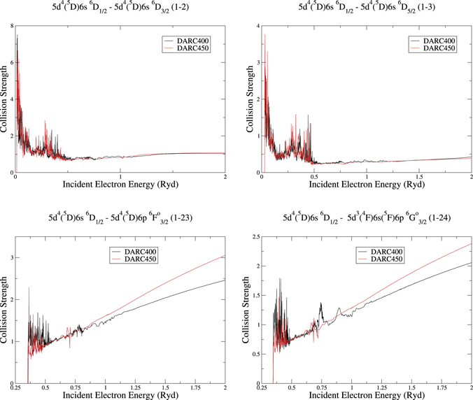
Figure 2. Collision strengths, from the DARC400 (model 2) and DARC450 (model 3) calculations, for the (top-left) 5d46s 6D1/2 to the 5d46s 6D3/2 (1–2), (top-right) 5d46s 6D1/2 to 6D5/2 (1–3), (bottom-left) 5d46s 6D1/2 to 5d46p 6
 (1–23), and (bottom-right) 5d46s 6D1/2 to 5d36s6p 6
 (1–24) lines respectively.
Download figure:
Standard image High-resolution imageFigure 3 present the effective collision strengths which correspond to transitions 5d46s 6D1/2–5d46s 6D3/2 (1–2, top-left), 5d46s 6D1/2–6D5/2 (1–3, top-right), 5d46s 6D1/2–5d46p 6
 (1–23, bottom-left), and 5d46s 6D1/2–5d36s6p 6
 (1–24, bottom-right) respectively for log Te
[K] = 3.0–6.0. For the forbidden transitions there is some divergence at low temperatures between the three calculations, however excellent agreement is seen between all calculations at higher temperatures. For the dipole interactions excellent agreement is shown between the DARC400 and DARC450 calculations, the DARC200 calculation deviates at higher temperatures. The more sophisticated models produce weaker collision strengths for these transitions. These variations arise due to differences in the target structures used. For the DARC200 calculation, the model 1 structure gives an A-value of 8.13 × 10⁷ s−1 compared to the value of 6.98 × 10⁷ s−1 for the model 2 structure in the DARC400 calculation and 5.58 × 10⁷ s−1 for the model 3 structure in the DARC450 calculation.
(1–24, bottom-right) respectively for log Te
[K] = 3.0–6.0. For the forbidden transitions there is some divergence at low temperatures between the three calculations, however excellent agreement is seen between all calculations at higher temperatures. For the dipole interactions excellent agreement is shown between the DARC400 and DARC450 calculations, the DARC200 calculation deviates at higher temperatures. The more sophisticated models produce weaker collision strengths for these transitions. These variations arise due to differences in the target structures used. For the DARC200 calculation, the model 1 structure gives an A-value of 8.13 × 10⁷ s−1 compared to the value of 6.98 × 10⁷ s−1 for the model 2 structure in the DARC400 calculation and 5.58 × 10⁷ s−1 for the model 3 structure in the DARC450 calculation.
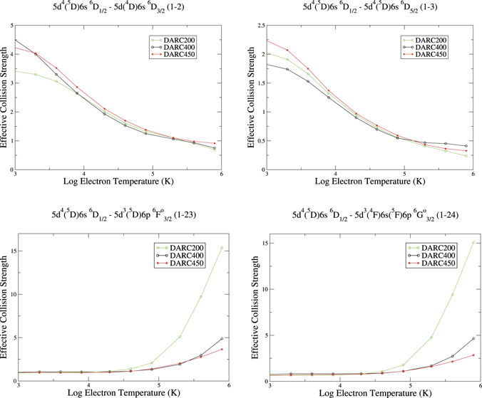
Figure 3. Effective collision strengths, from the DARC200 (model 1), DARC400 (model 2) and DARC450 (model 3) calculations, for the (top-left) 5d46s 6D1/2 to the 5d46s 6D3/2 (1–2), (top-right) 5d46s 6D1/2 to 6D5/2 (1–3), (bottom-left) 5d46s 6D1/2 to 5d46p 6
 (1–23), and (bottom-right) 5d46s 6D1/2 to 5d36s6p 6
 (1–24) lines respectively. Presented for log Te
[K] = 3.0–6.0.
(1–24) lines respectively. Presented for log Te
[K] = 3.0–6.0.
Download figure:
Standard image High-resolution imageTo provide a test for convergence, in figure 4 we present the transition from the ground state 5d46s 6D1/2 to the 5d46p 4P1/2 (1–22) state. We will follow this labelling convention throughout this paper for describing the transition from a lower level (1) to an upper level (22), corresponding to the final adf04 dataset. In this figure we show the collision strength computed with the inclusion of contributions from successively higher partial waves. There is a large contribution to the cross section from the partial waves between 2J = 0 and 20. Near convergence is achieved with the addition of the next 20 partial waves up to 2J = 40 and the resonance structures at low energies show excellent agreement. The contribution from partial waves  = 40 is clearly much smaller and shows that we have achieved near convergence. In fact including additional partial waves in the calculations would have a negligible effect. These Maxwellian-averaged effective collision strengths were generated from the collision strengths and the dataset will be made available.
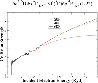
Figure 4. Collision strength for the 5d46s 6D1/2–5d46p 4P1/2 (1–22) line showing the successive contributions for 20, 40, and 60 partial waves.
Download figure:
Standard image High-resolution image4. Collisional radiative modelling
As detailed in the study by P tterich et al [4], tungsten erosion measurements are of the upmost importance to fusion reactors. In order to estimate the redeposition of tungsten spectroscopically, one needs W II and W I spectral lines. A complete analysis of which W II lines to be used for such diagnostics will be the subject of future work. However, in this paper we present some W II spectral comparisons with CTH spectral measurements as part of the benchmarking of the atomic data in this paper. Identifying W ii lines which lie in the same wavelength region as W i lines would allow for a redeposition investigation. W i lines have been identified in the 355–366 nm wavelength region by JET [34], therefore we have included this region in our analysis. To illustrate and draw comparison with observed sources of W ii we utilised the data computed in model 3 (DARC450 calculation). We built a collisional-radiative model [13] for W ii using the effective collision strengths from the electron-impact excitation calculation and the radiative transition probabilities from the atomic structure calculations. Forming a collisional-radiative matrix Cjk
requires both the electron impact excitation and radiative decay rates. This matrix is utilised to calculate photon emissivity coefficients (PECs), which for a particular transition (i → j), within the quasi-static approximation, can be described as the product of the radiative transition probability value (Einstein A coefficient) and the population of the upper level. PECs (in number of photons cm−3) are calculated as the following,
tterich et al [4], tungsten erosion measurements are of the upmost importance to fusion reactors. In order to estimate the redeposition of tungsten spectroscopically, one needs W II and W I spectral lines. A complete analysis of which W II lines to be used for such diagnostics will be the subject of future work. However, in this paper we present some W II spectral comparisons with CTH spectral measurements as part of the benchmarking of the atomic data in this paper. Identifying W ii lines which lie in the same wavelength region as W i lines would allow for a redeposition investigation. W i lines have been identified in the 355–366 nm wavelength region by JET [34], therefore we have included this region in our analysis. To illustrate and draw comparison with observed sources of W ii we utilised the data computed in model 3 (DARC450 calculation). We built a collisional-radiative model [13] for W ii using the effective collision strengths from the electron-impact excitation calculation and the radiative transition probabilities from the atomic structure calculations. Forming a collisional-radiative matrix Cjk
requires both the electron impact excitation and radiative decay rates. This matrix is utilised to calculate photon emissivity coefficients (PECs), which for a particular transition (i → j), within the quasi-static approximation, can be described as the product of the radiative transition probability value (Einstein A coefficient) and the population of the upper level. PECs (in number of photons cm−3) are calculated as the following,

The reduced collisional-radiative matrix  has the ground state row removed. For plasma diagnostics, in order to classify impurity influx [35] it is important to mention the sxb value, which is the ratio between the effective ionisation rate Sz→z+1 and the photon emissivity coefficient for transition i → j. This sxb ratio is defined as,

where the effective ionisation rate encapsulates the ground and excited state ionisation. The impurity influx Γ incorporates the sxb ratio as follows,

As the sxb ratio is dependent upon data from ground, metastables, and excited states, classifying this impurity influx is particularly difficult for heavier elements where time-dependent metastable populations may be important. Therefore, it is beneficial to have both experimental observations and theoretical data.
The DARC450 data was incorporated into the ColRadPy collisional-radiative modelling code [14] to model the spectra of W ii to help identify potential diagnostic lines. Of particular interest are the wavelength regions which overlap between neutral and singly ionised tungsten. We do not consider the effects of metastable states on the level populations in this work, however this may be explored in future work.
The CTH plasma experiment [36] located at Auburn University provided tungsten emission measurements for comparison with the dataset presented in this paper. A high-resolution, UV optimized spectrometer observed emission between 200 and 400 nm from plasma–tungsten interactions. The experiment involved inserting a vertically translating tungsten tipped probe into the edge of the CTH plasma, spectrometers are coupled by an optical fibre to collection optics focussed on the tungsten tip. The temperature at the probe tip is expected to be within the 10–30 eV range and the electron density to be  cm−3. We note that many W I and W II lines occur in the spectra, along with impurity lines largely due to B, C, O, and N.
Figure 5 presents the results from the current model compared to observations from the CTH experiment across the 216–227 nm and 243–253 nm ranges. In the 216–227 nm wavelength range, we see that the 5d46s 6D5/2–5d36s6p 6
 (218.22), 5d46s 6D3/2–5d46p 4
 (218.93), 5d46s 6D7/2–5d46p 4
 (224.52), 5d46s 6D1/2–5d36s6p 6
 (224.88), and 5d46s 6D5/2–5d46p 6
 (225.07) transitions all exhibit reasonable agreement, in terms of both spectral height and wavelength. These lines are observed in both the work of Ekberg et al [21] and Kling et al [23]. The upper identifications of the 218.93 nm and 224.52 nm lines have not been previously identified, however the identifications we have listed are of the correct energy, and Jπ symmetry. The A-values of the 218.93 nm and 224.52 nm lines from our dataset are 3.63 × 10⁷ s−1 and 3.83 × 10⁷ s−1, respectively, showing agreement with the observations of Kling et al [23], who recorded A-values of 4.33 × 10⁷ s−1 and 4.91 × 10⁷ s−1, respectively.
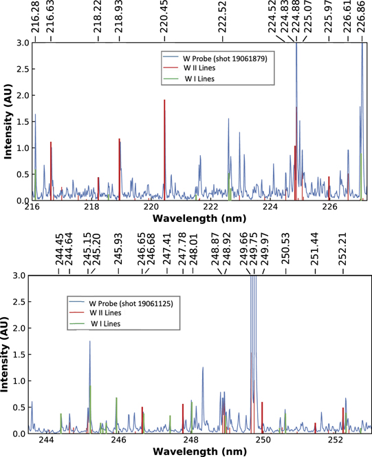
Figure 5. Observed spectra from the CTH experiment (solid blue line) compared to the present theoretical results between 216–227 nm (top) and 243–253 nm (bottom). Vertical red and green sticks are the relative PECs for W ii and W i, respectively, for an electron temperature of 8 eV and electron density of 1 × 1012 cm−3.
Download figure:
Standard image High-resolution imageThere are several lines which display reasonable agreement between the CTH experiment and the DARC450 calculation; however, these lines have not been previously identified with both the lower and upper levels and have no radiative data to compare with. The lines however have been observed in the work of Ekberg et al [21]. All level identifications for these lines are of the correct energy, and have the correct Jπ symmetry. The following lines have been identified using the limited information available; the 5d46s 6D7/2–5d46p 6
 (216.63), 5d46s 6D9/2–5d36s6p 6
 (220.45), 5d46s 6D7/2–5d46p 6
 (224.83), 5d46s 6D5/2–5d46p 4
 (225.97) and 5d46s 6D7/2–5d46p 6
 (226.61) transitions. The W i lines presented in this plot have been produced by Smyth et al [11], however there is no comparative data in existing literature to confirm these lines. There is agreement with CTH spectra, which gives us confidence in the results.
The bottom plot of figure 5 presents spectral plots of W ii in the 243–253 nm wavelength region. We identify the following spectral lines; the 5d56S5/2–5d46p 4
 (244.64), 5d46s 6D3/2–5d46p 6
 (245.15), 5d46s 6D3/2–5d46p 6
 (246.65), 5d46s 6D9/2–5d36s6p 6
 (247.78), 5d56S5/2–5d46p 6
 (248.87), 5d46s 6D7/2–5d46p 6
 (249.65), 5d46s 6D9/2–5d46p 6
 (249.75), 5d56S5/2–5d46p 4
 (249.97) and 5d56S5/2–5d46p 4
 (251.44), and 5d46s 6D5/2–5d46p 6
 (252.21) transitions. When compared to the CTH experiment the data exhibits reasonable agreement in terms of position and height for all lines listed. The upper level identification for the 245.15 nm, 249.66 nm and 251.44 nm lines has not been identified in the literature, and the lower level identification has not been completed for the 252.20 nm line, however our identification agrees with the energy and Jπ symmetry listed. These lines have been observed and radiative data recorded by Kling et al [23]. The 244.64 nm, 249.75 nm, and 249.97 nm have no radiative data in existing literature for comparison, however the energy and Jπ symmetries agree for each line. As our data displays good agreement with the CTH experiment we are confident in identifying these lines. This region also contains W i lines, identified at 244.45 nm, 245.20 nm, 246.68 nm, 247.41 nm, 248.01 nm, and 250.53 nm, which agree with the results presented by Kling and Kock [37].
Figure 6 presents the spectral plots of W ii in the 360–365 nm wavelength region. Previous investigations have focussed on diagnostics in the visible region, so it is important to compare within this region to give additional confidence in the results. This region also contains W i lines, for example there is a feature observed at 361.71 nm in the CTH experiment data which is identified as a W i line and agrees with the result of van Rooij et al [34]. Also the 363.19 nm line agrees with the observed results of Hartog et al [38]. Identifying both neutral and singly ionised tungsten in the same region would prove useful for a redeposition investigation, particularly lines which are not blended with each other. The 364.14 nm (5d36s24F3/2–5p65d46p 4
 ) and 364.56 (5p65d46s 4D5/2–5p65d36s6p 6
 ) both display good agreement with the experimental observations, and the corresponding radiative data also agrees with the experimental results recorded by Ekberg et al [21].

Figure 6. Observed spectrum from the CTH experiment (solid blue line) compared to the present theoretical results between 360–365 nm. Vertical red and green sticks are the relative PECs for W ii and W i, respectively, for an electron temperature of 8 eV and electron density of 1 × 1012 cm−3.
Download figure:
Standard image High-resolution image
The main purpose of the CTH comparison shown in this section is to check that the strong W ii lines observed in CTH are also predicted from the atomic data calculated here, when used in a collisional-radiative model. For a detailed study, investigating time-dependent metastables and the role of neutral W on the modelling of W ii spectra, a more complex model should be constructed. It has already been shown for neutral W [39] that time-dependent modelling of metastable states may be required to accurately predict the line intensities of W i lines that decay to metastable levels. In the current model, the metastable states are assumed to be in steady-state conditions with the ground, i.e., the quasi-static approximation. In addition, it seems reasonable that the excited states of W+ may be significantly populated from ionization of metastable and excited states of neutral W, for which no data currently exists. The reasonable agreement of the current model with observed CTH spectral lines indicates that the bulk of the populating mechanisms for the excited states of W+ is likely to be collisional excitation within W+. However, future work should include a model that simultaneously includes time-dependent metastable modelling of both neutral W and W+.
5. Conclusion
The atomic data reported here represents the most comprehensive dataset for electron-impact excitation of W ii currently available. Three atomic structures have been created, an initial structure (model 1) contained 8 configurations. The larger structures, model 2 and model 3, contained 13 and 17 configurations in the description of the target ion, respectively. The fully relativistic DARC R-matrix packages were utilised in the collision calculations. Comparisons were made with experimental observations in the works of Ekberg et al [21], Lennartsson et al [26], and Quinet et al [25] between the A-values for many transitions. It was found that model 3 was in agreement with observed values.
Collision strengths were evaluated for all transitions, both forbidden and allowed, between the lowest 400 fine structure levels for incident electron energies up to 2 Rydbergs. Careful attention was given to ensure the Rydberg resonances were resolved and the high partial wave contributions were converged. In accessing the accuracy of the collision strengths, three calculations were completed, a 200 jj-level (model 1: DARC200), a more substantial 400 jj-level (model 2: DARC400), and a 450 jj-level (model 3: DARC450). The corresponding Maxwellian averaged effective collision strengths were evaluated for a large range of electron temperatures log Te [K] = 3.0–6.0. Excellent agreement was achieved for the forbidden lines between all calculations, however the dipole lines showed a greater divergence due to the differences in the atomic structure models. The data set presented in this work represents the most comprehensive calculation to date for W ii and will be available in adf04 format in the ADAS database [40].
Through the use of extensive collisional-radiative modelling and the incorporation of the results from both the atomic structure and collisional models, a synthetic spectra for singly ionised tungsten was produced. Comparisons were drawn between relative intensities and wavelength using recent measurements from the CTH experiment. These spectral line diagnostics will help characterise the impurity influx predictions of W ii in fusion relevant plasmas. It is hoped that model 3 and the subsequent collisional calculation DARC450 will provide insight for future experiments and identify a single wavelength window in which both W i and W ii emit strong emission lines to be used for diagnostic purposes. In addition, it is hoped the dataset will be useful for redeposition studies.
The effective collision strengths produced here will be made available in an adf04 file via OPEN-ADAS at http://open.adas.co.uk/.
Acknowledgments
This work is supported by funding from the STFC ST/P000312/1 QUB Astronomy Observation and Theory Consolidated Grant. This work was also supported by the Prof. James Caldwell Travel Scholarship, and the experimental data was funded by US Department of Energy Grants DE-SC0015877 and DE-FG02-00ER54610. This work used the ARCHER UK National Supercomputing Service (http://archer.ac.uk), the Cray XC40 Hazel Hen supercomputer at HLRS Stuttgart, Summit at ORNL and a local cluster at Queen's University Belfast. We would like to acknowledge R T Smyth for contributions towards the structure and write up of this work.
Data availability statement
The data that support the findings of this study are available upon reasonable request from the authors.