

Abstract
A good experimental task for a high school physics competition requires an interesting and relatable topic, careful testing, and meeting constraints of time, budget, and curriculum. This article presents the experimental task from the European Physics Olympiad in the year 2022. The students explored the properties of light sources, such as their colour temperature, angular light distribution, efficacy, and heating. The task was stated without explicit instructions, inviting the students to devise their own approach to measurement and data processing. The original task was designed for a level slightly above the European high-school curriculum, so parts of it can be directly used as a lab exercise at a university level or simplified and given more specific instructions for inclusion in high school level education.
Export citation and abstract BibTeX RIS

Original content from this work may be used under the terms of the Creative Commons Attribution 4.0 licence. Any further distribution of this work must maintain attribution to the author(s) and the title of the work, journal citation and DOI.
1. Introduction
The European Physics Olympiad (EuPhO) was introduced in 2017 with the goal of bringing shorter and more challenging tasks [1] in comparison to other international competitions [2]. The chosen task, solved by individuals, consists of a theoretical and an experimental part, both with a five hour allotted time. The tasks only state the required results without explicit instructions, so the students must apply their knowledge to devise the approach to the solution. The tasks are kept secret from the participants before the competition and are revealed only by handing out the task sheets at the start of the allotted competition time. In May 2022, the EuPhO took place in Ljubljana, Slovenia [3]. It was attended by 182 high school pupils from 37 countries. It is notable that only 16 participants were female, showing a large gender disparity within applicants of this competition.
The theoretical tasks were prepared by the international academic committee, while the experimental tasks (figure 1) were prepared by the local academic committee. Preparation of the tasks by the local academic committee started two years before the competition, when the exact number of participants was not yet known, and consisted of the selection of a preliminary topic, followed by an evaluation of feasibility and scalability. The experiment had to be designed in such a way that it was (a) financially feasible to acquire about 200 experimental sets, including extra sets for testing and redundancy, and (b) that the activity filled a five-hour time period. During this development phase, the intensive testing of the task draft took nine months, followed by selection and purchase of required equipment and performing repeated tests under different conditions to ensure reproducibility and to gather statistics for appropriate grading. During this phase, we also improved upon the design of the prototypes of the custom-developed experimental materials. Prototypes were made by 3D printing, and the final version was laser-cut from plywood. The text of the tasks was improved following test evaluations by students, which helped us find ambiguous or unclear parts of the questions through the examination of their solutions.
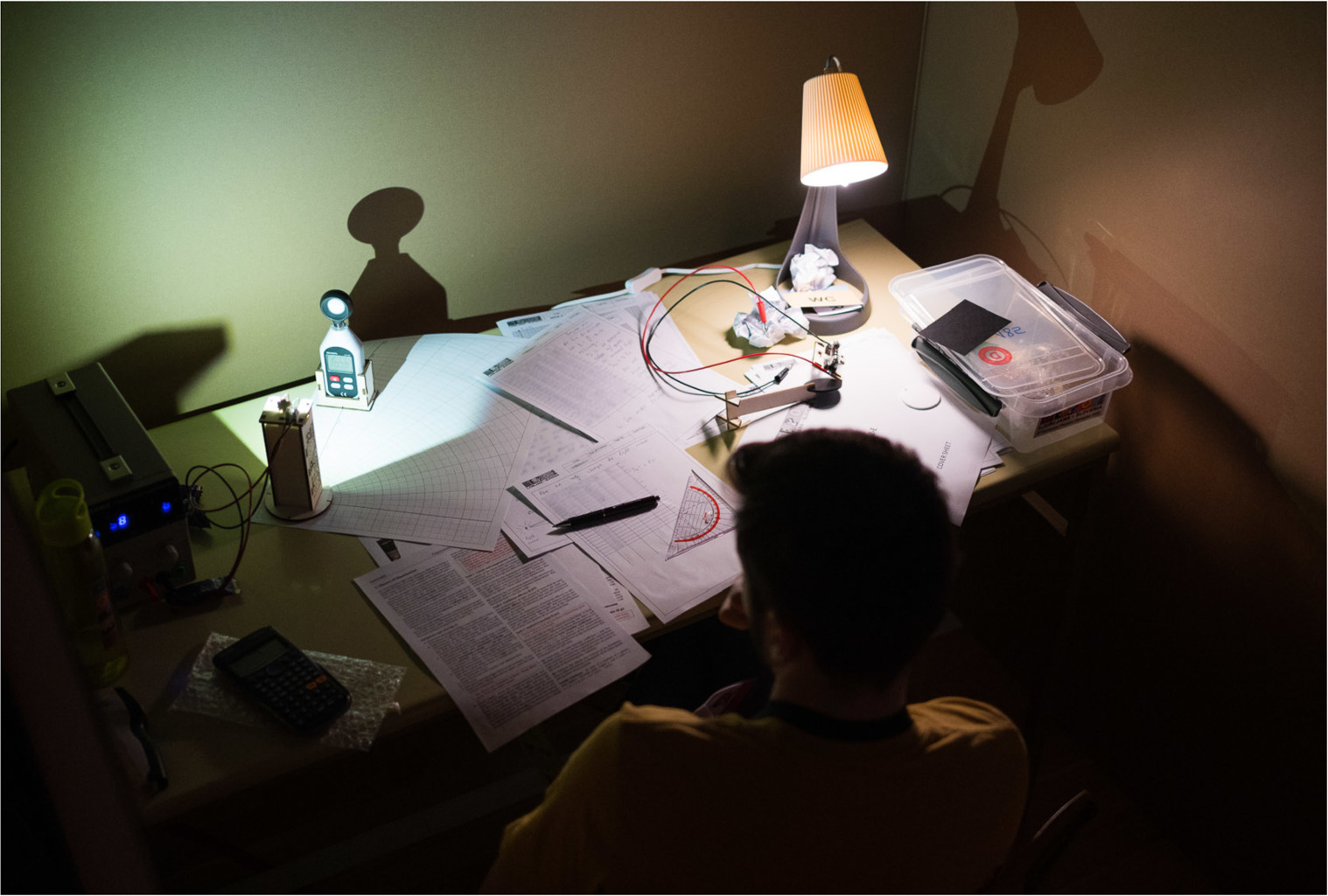
Figure 1. The experimental station at the competition. The experiment was performed in a darkened gymnasium to eliminate ambient illumination in photometric measurements. Photo: Jan Šuntajs.
Download figure:
Standard image High-resolution imageIn this manuscript, we present the idea behind the experiment, which was centered broadly around illumination and more specifically around properties of light sources. We discuss the tasks not only as a part of the competition but as components that can be reused by readers directly or in a modified form. We anticipate that the tasks could be adapted for use in the classroom, training lessons before physics competitions, workshops, and other hands-on events. For that purpose, we discuss the physics knowledge involved in solving each task, the reasoning required to devise an appropriate path to the solution, and different experimental approaches that lead to accurate results.
2. The topic
Light and its physical properties in the context of illumination are an ever-present part of our lives—in indoor lighting, photography, art, road safety, and displays of personal electronic devices. In indoor illumination, we must pay attention not only to the light intensity but its distribution in the room, possible overheating, power consumption efficiency, and faithfulness of colour reproduction. All these parameters play important roles in the usability of light sources and their effect on our safety and comfort.
Throughout most of human history, we relied on incandescent light sources, such as sunlight and flame. Since the commercial success of Edison's light bulbs in 1879, electric lighting entered our homes and replaced previously widespread combustion-based light sources. A modern incandescent light bulb uses a thin tungsten filament heated to a high enough temperature for it to glow as a black body in the visible part of the spectrum. Such light sources dissipate a lot of energy through the emission of invisible infrared light, which constitutes a significant part of the black body spectrum. This low efficiency spurred the development of more efficient lighting technologies, such as fluorescent tubes, compact fluorescent lights, and LED lights. For household use, especially with the increasing importance of energy saving, it is imperative to reduce energy losses, where waste heat and light emissions outside the bounds of human vision present two major contributions. Simultaneously, the spectrum of light must be optimised to still look white and to make the illuminated objects appear similar to the human eye as in daylight. In light source specifications, this property is measured by the colour rendering index (CRI) [4].
An important side-effect of incandescent emitters is the heating of the surroundings via absorption of the infrared emissions. Incandescent light bulbs cause significant heating of the light fixture and nearby furniture and walls and consequently contribute to the heating of the room. The effect depends on the albedo (reflectivity) of the surface in the relevant range of wavelengths. For example, the Sun heats dark vehicles more than light-coloured ones and also causes the urban heat island effect by heating the dark asphalt and concrete surfaces. For incandescent light bulbs, we can judge from the peak around 1 μm in the spectrum in figure 2, that absorption in the near-infrared range is the main factor in the heating effect. In the visible part of the spectrum, absorption is determined by colour, and we can raise the question of whether black and white objects also differ in absorption in the near-infrared range.

Figure 2. Comparison of the LED spectrum, reference incandescent bulb spectrum (Thorlabs SLS201L [5]), and ideal black body spectra at three temperatures. Incandescent light sources emit a lot of light in the infrared range.
Download figure:
Standard image High-resolution image3. The tasks
The experiment was crafted so that competitors could relate their everyday experience about light source efficiency and the effects of albedo on surface temperature with quantitative measurements of photometric, radiometric, and electrical quantities. They could experiment with different aspects of light sources and familiarise themselves with the physical characteristics of light.
The nature of the experiment required the competition to take place in a dark environment. Daylight was blocked by covering the windows of the gymnasium where the competition took place. The possibility of stray light from other competitors to disrupt the measurements was mitigated by enclosing each competitor in a tall cardboard cubicle from 3 sides. For writing and reading, they were provided with individual desk lamps which they could, and in fact should, turn off during measurements (figure 1).
The experiment consisted of three tasks, with 5 h of allotted time. In this section, we will present the tasks in the descriptive form. The full original instructions, solutions, and grading schemes can be found in the official repository [6]. Detailed equipment specifications and resources required to reproduce the experiment are freely available online [7].
In this section, we will discuss each task in more detail. The instructions for each task were short, leaving the decisions of how to measure and process the data to the participants. They had to choose the correct assumptions, familiarise themselves with the workings of the experimental devices, and design the experimental procedure. The experimental equipment they were provided with is shown in figure 3. Special attention had to be given to using the tabletop power supply, which doubled as a voltage or current meter. The kit was selected to keep the cost within the constraints of the event budget, which also makes it affordable for hands-on experiments in high schools.
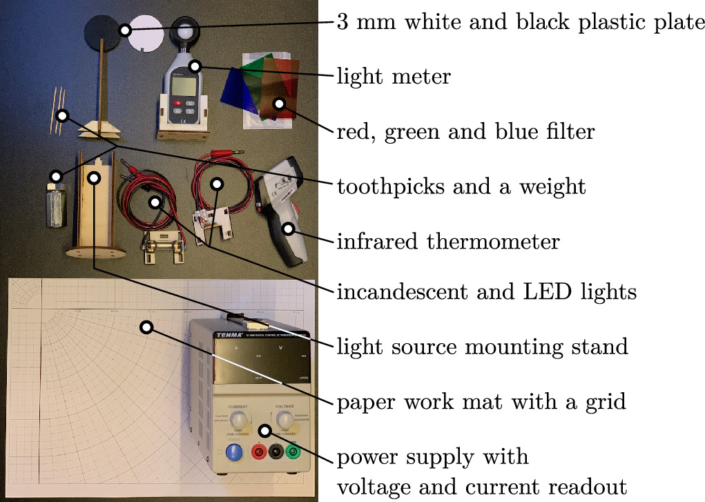
Figure 3. A full set of experimental equipment provided to the competitors. The toothpicks and a weight were provided to stabilize the light source mount against the torque of the stiff wires.
Download figure:
Standard image High-resolution imageThe open-ended approach, favoured by the EuPhO competition [1], is in line with modern approaches to laboratory activities in physics education [8, 9]. A shift from guided experiments to experiments that engage students in experimental design shows improvements in both knowledge and confidence in experimental work post-instruction [10]. Through experimentation, an interest in the observed phenomenon is increased, resulting in a productive motivation of the student [11]. To obtain the results and thus construct the answers to the task, the students had to improve upon the simple observation by constructing a set of appropriate hypotheses and assumptions on which to base their experiments. Performing the experiments that should either confirm or disprove their hypothesis required getting acquainted with the realistic experimental equipment and thus assisted in building transferable technical skills. These design considerations, in fact, are well aligned with the inclusion of the experimental task in classrooms.
Should one undertake the translation of the task into the classroom or physics laboratory, the equipment needed is either affordable or already available at the school or university. The full list of equipment used for the experiment is available in the official repository [6] and depicted in figure 3. In brief, one should have access to a power supply with integrated voltage and current meters, light bulbs with appropriate symmetry (in the official materials, a car light bulb with rotational symmetry and an ordinary SMD LED were used), as well as a means to measure light intensity (a light meter) and temperature (preferably an IR contact-less thermometer). To observe the heating of materials, different samples could be used, but for the official task, white and black circular samples of foamed PVC material (forex) were used. In the official repository, the plans for the specialised components for light-bulb and instrument positioning are available, but these can be easily replaced by common clamps and other basic laboratory equipment.
3.1. Colour temperature
Incandescent light sources emit light with a spectrum approximately following the Planck's law of black body radiation (figure 2). The wavelength at which the spectral density of the light is the highest is decreasing with increasing temperature in accordance with the Wien's displacement law, from red and orange towards the blue part of the spectrum, which is directly observable from the colour of the emitted light. The temperature of black body emissions uniquely determines its colour, so it is a good parameter to quantify it. We use the term colour temperature to describe the colour of a light source, even for non-incandescent light sources, such as fluorescent and LED lights, in order to specify which temperature of black body radiation it most closely resembles.
Quantitative description of light, as seen by the human eye, is encapsulated by photometric units, which are scarcely included in the high school curriculum. Thus, a brief review is needed: the total amount of light, emitted by a source into all directions, the luminous flux, is measured in lumen [lm]. The received light per unit of area is called illuminance, measured in lux [lx = lm/m2]. This is the quantity measured by the light meter, which was provided in the kit. There are other photometric quantities that also relate angular information, but they will not be needed for this task [12–14].
In astronomy, the brightness of stars is measured in magnitude, which is logarithmically related to the light intensity measured by detectors. The colour of stars is quantified by the colour index, the difference of magnitudes measured through two filters, such as the B–V index for the difference between magnitudes through blue (B) and yellow-green (V stands for visible) filters, which is analogous to a quotient of corresponding intensities [15]. With proper calibration, colour index can be used to determine the temperature of the star [16–18].
The same method works for determining the temperature of other objects [19], which was used by the competitors in their first task. They were to determine the temperature of the light bulb filament at different powers. The temperatures are too high to be measured using conventional thermometers. Three filters were provided—red, green, and blue—and a light meter, making it possible to measure the detector illuminance through different filters. They had to prepare a calibration curve based on the provided table, which we are showing in figure 4(a) in graph form.
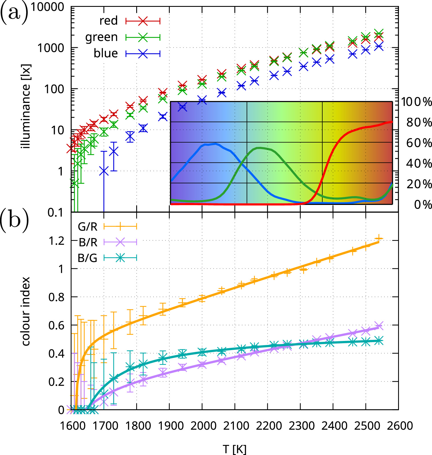
Figure 4. (a) Raw data for the colour intensity of an incandescent light bulb with a filament at a known temperature, measured through three filters. The students were given this data in the table form. The inset shows the transmittance spectra of the filters between 400 and 700 nm. (b) Calculated colour indices (quotients of filter pairs). We can deduce that using the red and green filters is best for accurate determination of temperature due to the steepest trend.
Download figure:
Standard image High-resolution imageThe first task, adapted for stand-alone clarity, was as follows:
Task 1—Colour and temperature
The colour of the black body radiation depends on its temperature. In astronomy, the temperature of stars is determined from their colour index, the ratio of illuminances measured through two different colour filters.
- (a)Illuminance of a standard incandescent light source at different temperatures measured through red, green, and blue colour filters is provided. Pick an appropriate pair of filters and construct a calibration curve that relates the chosen colour index to temperature.
- (b)Measure the relationship between the input electrical power and the temperature of the tungsten filament. Plot the relationship across the relevant range.
The objective was to select only two filters to measure an associated colour index. While it is possible to make an acceptable measurement using any pair of filters, an inspection of the data shows that values through green and blue filters follow similar curves, so their quotient spans across a narrower range, and a small error in the colour index would result in large uncertainty in temperature, as shown in figure 4(b). Using a red filter in combination with one of the other two is thus a more suitable choice. Additionally, the values obtained through the blue filter are much dimmer and thus carry a larger uncertainty; therefore, the red and green pair was the best choice. With the exception of the lowest temperatures, the calibration curve can be approximated with a linear relationship, which simplifies conversion.
Figure 5 depicts the experimental setup. The distance to the light meter should be the same for both filters to avoid the effect of the inverse square law and directional intensity profile. The filter must cover the entire light meter sensor. Careful measurement yields an expected relationship—the filament temperature increases with power, but not linearly [see figures 5(b), (c)]. Avid students might also notice that the trend roughly follows a model

which is shown as a dotted line in figure 5(c). This holds under the assumption that all the power is radiated away as black body radiation following Stefan-Boltzmann law, neglecting convection and the radiation received from the surroundings. At the high temperatures reached by the filament, this is a reasonable assumption and can, in fact, be confirmed by using a bolometer to measure the total light flux emitted by the tungsten filament and comparing it to the values of electrical power consumed.
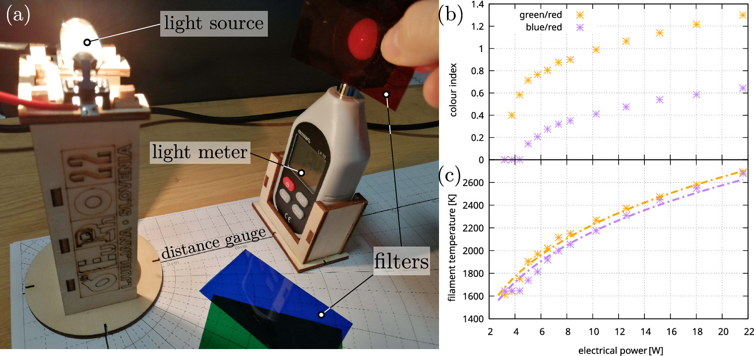
Figure 5. (a) Experimental setup for measuring the colour temperature. (b) Colour indices calculated from the pairs of measurements through filters at the lightmeter-source distance 10 cm. The distance in the panel (a) image is larger for presentation purposes. (c) Data converted into temperatures based on the calibration graph 4(b). Dotted line is based on the Stefan-Boltzmann law model. Observe that different filter pairs give somewhat different answers, indicating that the results are only reliable up to ±100 K.
Download figure:
Standard image High-resolution imageOne of the notable mistakes made at this task was to place the filter on the light bulb instead of the light meter, despite the warning on the instructions. Some students misunderstood the instructions, assuming they should recreate the given calibration table themselves by measuring the temperature using the IR thermometer.
3.2. Light source efficacy
Luminous efficacy is the ratio between emitted (visible) luminous flux and the emitted power. For example, sunlight has an efficacy of 93 lm W-1 [20]. For electric light sources, input electrical power is usually used as the denominator, as it is easier to measure and more relevant for power consumption considerations.
The second task asked for the efficacy of two light sources in relation to the input power: an incandescent light bulb and an LED. It is easy to assume that the LED will be more efficient, but the dependence of the efficacy on how they are driven is less intuitive. A quantitative result requires careful measurements and taking geometry into account, as outlined in the task statement:
Task 2— Luminous efficacy
The performance of light sources is quantified by their luminous efficacy, as the ratio between the luminous flux and the consumed power. As a point of reference, the Sun has a luminous efficacy of 93 lm W−1.
Measure the dependence of the luminous efficacy on the electrical power for both provided light sources across the range of detectable light outputs. Plot the dependence for both sources and document your measurement procedure.
To estimate the luminous flux, the light meter must be placed perpendicular to the light direction, eliminating the geometric effect of oblique light incidence. Thus, the measured illuminance E is just equal to the luminous flux density [lm/m2] at that position. For a light source that shines equally in all directions, the luminous flux could be obtained by multiplication of the measured illuminance at distance r by the area of the sphere: Φ = 4π r2 E. In our case, this does not suffice, as our light sources are not isotropic. Instead, we can imagine enclosing our light source into a sphere and summing contributions to the flux Φ[lm] over small patches we assume have approximately the same flux density, each multiplied by the patch area (see figure 6). Thus, we account for all the rays and get the entire flux. Mathematically speaking, this is an integral over the solid angle Ω:

but for the purposes of this task, it will be evaluated as a discrete sum over measurements, so knowledge of integrals is not required.
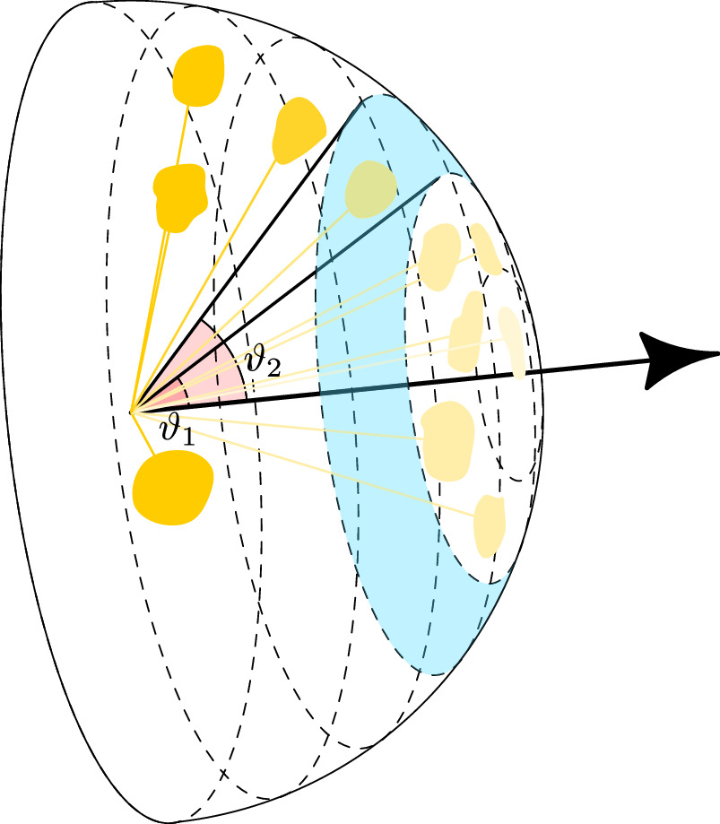
Figure 6. Luminous flux density varies with direction. Instead of summation over all spatial directions, we can use the symmetry to sum over spherical annuli (e.g. blue shaded part between angles ϑ1 and ϑ2).
Download figure:
Standard image High-resolution imageWe notice that the provided incandescent bulb is cylindrical, with the rotational symmetry axis perpendicular to the forward direction. The LED also has rotational symmetry, but pointing along the forward direction instead. Additionally, the LED emits no light in the backward direction [see figure 7(a)]. Rotational symmetry was a strict constraint for the selection of the light sources for the task because the general asymmetric case makes experimental realisation infeasible and complicates the mathematical process of obtaining the total light flux.

Figure 7. (a) Close-up images of both light sources, showing their rotational symmetry. (b) Experimental setup for measuring the angular profile of the luminous flux with data points and error bars at 9 angles in a single quadrant. LED only emits into half of the space, and is symmetric around the centerline, while the incandescent bulb emits in all directions and is symmetric under rotations around a perpendicular axis (the direction of the filament). The dotted line shows a simplified model of the angular dependence. The shadows seen on the mat are not problematic for the light meter, which is aligned at the height of the light. (c,d) Efficacy of the incandescent bulb (c) and the LED (d) in relation to the input power. The increased slope at P < 0.1 W for the LED (d) is an artefact of inaccurate current regulation at very low currents—there is a small bias current even when the readout is at zero.
Download figure:
Standard image High-resolution imageThis insight indicates we only have to measure the illuminance in the plane of the desk, along the circle from the forward direction to the perpendicular direction [measurements in these directions are shown in figure 7(b)], instead of measuring in all spatial directions. The calculation relies on the area of a spherical annulus between ϑ1 and ϑ2, which is  (see figure 6). This equation was provided as a mathematical hint in the task. Care is required in interpreting the angle ϑ, because the light sources have differently oriented symmetry axes. The competitors had to estimate the number of angular divisions that suffice for a reasonably accurate result. Some competitors chose to measure symmetrically in both directions from the forward direction, which improves the accuracy by accounting for departures from the assumed symmetry, such as a poorly aligned light source and the tilt of the tungsten filament.
The angular measurement only has to be performed once for each light source; we can assume that varying the power only varies the intensity, not the angular distribution of light. Therefore, the ratio between the forward illuminance (E) and the total flux (Φ) does not change and can be determined with a single series of measurements. This gives us a nondimensional factor C in the expression of the form Φ = Cr2 E, where it replaces the specific value 4π that would hold for an isotropic light. All further data for the power dependence can then be measured only in the forward direction by changing the current on the power supply.
The factor C can also be estimated analytically based on the simplified geometry of the emitter. The LED can be assumed to be a flat Lambertian emitter, so the illuminance measured in each direction is proportional to  , leading to CLED = π. In our particular choice of the LED, the values obtained from experiments were somewhat smaller but within the range of variation CLED = 3.0 ± 0.2. Note that this is half the naive factor of 2π, which only accounts for the fact that LED only emits into half of the space. For the incandescent bulb, assuming an ideally thin straight Lambertian filament, the illuminance is proportional to
  , with ϑ measured from the cylinder axis. We obtain CW = π2, which matches the measured value of CW = 10.0 ± 0.3 quite closely. Competitors who attempted this path were graded equally for the part of the grade dedicated to obtaining the correct coefficient C.
Figure 7(b) depicts the angular profile of the luminous flux density for both light sources, with the luminous efficacy graphs shown in panels 7(c), (d). We notice that the efficacy of the incandescent light increases with power. The previous task suggests that increased power also increases temperature, which maximises the amount of power emitted in the visible part of the spectrum. Unfortunately, the temperature is limited by the melting point of tungsten at 3695 K, while the usable range is even lower due to material softening and evaporation of metal atoms into the bulb.
With the LED, the trend is reversed. Increasing the power reduces efficacy, mostly because of overheating, which reduces the quantum efficiency of the LED (a phenomenon known as thermal droop). An interested reader can find more information in the literature [21, 22]. The takeaway lesson is that for good efficacy, LEDs must be driven with moderate currents or at least be adequately cooled, which also helps increase their longevity. As expected, even in the worst case, LED is much more efficient than an incandescent light bulb.
Note that the prominent divergence of efficacy at the lowest powers is an artefact of the small bias current measured to be around 5 mA that flows even at zero readouts on the power supply. Consequently, the powers calculated from Ohm's law are too low, and after division, lead to overestimated efficacies. The measurements at powers below 0.1 W are thus unreliable.
The most common mistake in this task was the failure to realise that the angular profile of the emitted light must be measured or estimated analytically, leading to a very poor estimate of efficacy. Other issues were related to incorrect angle-dependent weights in regard to the rotational symmetry and the provided geometric hint.
3.3. Radiative heating
Illuminated objects get hotter. When the light falls onto an opaque object, a part of it is scattered away while the rest is absorbed and converted into internal energy. Ideal black bodies absorb all the incident light, while ideal white bodies scatter all the light and absorb none. Realistic cases lie in between these two scenarios, with dark bodies absorbing the majority of incident light, at least in the visible part of the spectrum. An object reaches thermal equilibrium when the losses into the environment due to conduction, convection, and radiation balance the radiant energy received through the illumination. For moderate temperature differences, we can assume that the losses are proportional to the temperature difference, P/A = h(T1 − T0), where h is the heat transfer coefficient and includes both convection and radiation. T1 is the temperature of the surface, and T0 the temperature of the surroundings. Because the surroundings are at different temperatures, and not necessarily at the temperature of the air, we must understand T0 as an effective temperature at which the object would equilibrate if no light was present. P/A is the dissipated power per surface area.
Not all the heat is lost from the front plate surface into the environment. A part of the heat is conducted through the plate and dissipated there. A plate with thickness d conducts  of power through it, where T2 is the temperature of the dark side of the plate, and λ is the thermal conductivity.
The third task was about determining these material parameters for the provided black foamed PVC in the shape of a circular disc with thickness d = 3 mm:
Task 3—Radiative heating
When light hits an object, some of it is absorbed. At moderate temperature differences between the object and the environment, we can model heat dissipation into the surroundings with the heat transfer coefficient h, in the form P/A = h(T − T0), where T is the temperature of the surface, T0 the temperature of the surroundings, and P/A denotes the power lost to the environment due to dissipation, per unit area.
- (a)Determine the thermal transfer coefficient h and thermal conductivity λ of the black plastic and perform uncertainty analysis. Assume the plastic absorbs all incident light and that the light bulb converts all electrical power into radiation.
- (b)Estimate the albedo (the fraction of the irradiance that is reflected instead of absorbed) of the white plastic.
This task is not concerned with human visual perception of light but with the actual energy carried by the light, regardless of its wavelength. Thus, we are using radiometric quantities, which are expressed with the conventional units of power. The radiometric analogue of the luminous flux is the radiant flux [W], and the analogue of illuminance is irradiance [W m–2], which equals the radiant flux density at perpendicular incidence.
The relations involving the unknown coefficients indicate that we need to quantitatively determine the equilibrium temperatures of the plate as well as the incident radiant flux. Figure 8(a) shows an experimental setup. The front and back temperature of the plate can be measured with the provided IR thermometer—both are needed to extract the thermal conductivity λ, which depends on their difference. The power balance for the front and the back surface, accounting for the incident flux, dissipation into the environment, and exchange due to conductivity, yields the following set of equations:


We are faced with the problem of how to extract h and λ out of the temperature measurements. Avoiding complex numerical procedures, the easiest way is to reinterpret the problem as finding the slope of a line. There are various different approaches—one is to take the sum and the difference of the above equations:


In this form, the coefficient h can be read out directly as the slope of the flux density j with respect to the sum of temperatures of both sides of the plate [see figure 8(b)], whereas λ requires an extra algebraic step [see figure 8(c)]. Forgetting the contribution of h to the temperature difference would lead to an overestimate of the thermal conductivity.
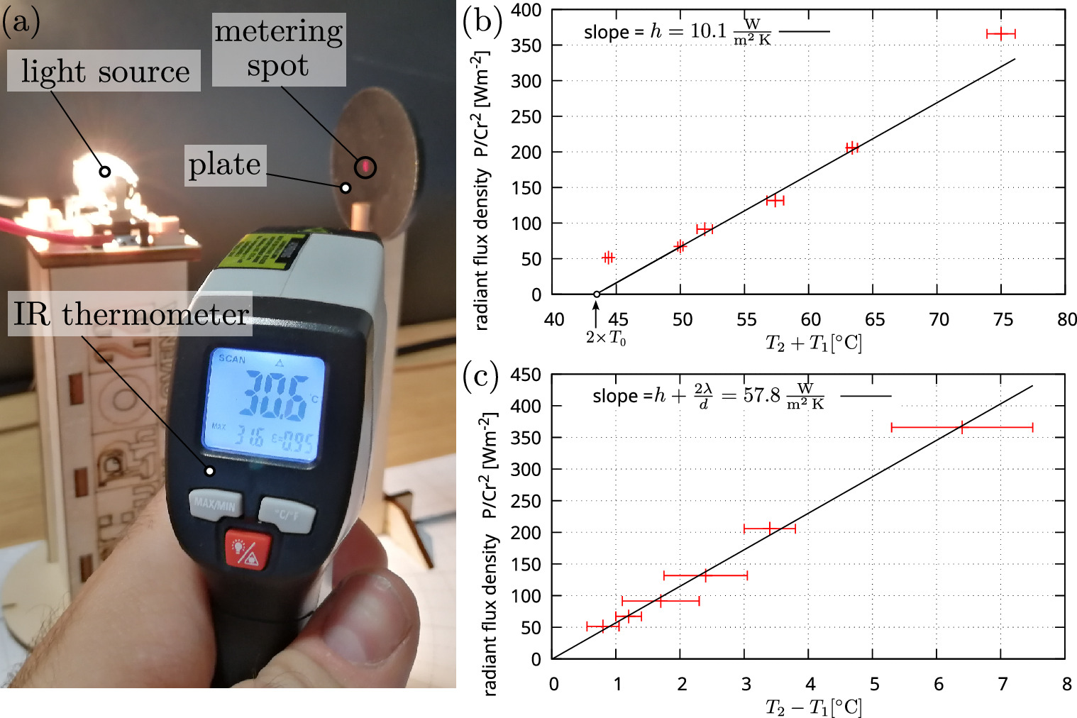
Figure 8. (a) Experimental setup for measuring the temperature of the plastic plate. The built-in laser of the IR thermometer helps to aim the instrument at the centre of the target. (b,c) The graphs of the sum and the difference of the front and back sides of the black plate. The vertical axis measures the radiant flux densities calculated from the power, the distance, and the geometric factor. The slope of graph (b) gives the thermal transfer coefficient, and the slope of (c) gives a weighted sum of the transfer and conductivity coefficient. Graph (b) suggests the effective surrounding temperature is around T0 ≈ 22 °C.
Download figure:
Standard image High-resolution imageThe effective external temperature T0 is difficult to measure, as it is a consequence of radiative and convective exchange with surrounding objects and walls that are not necessarily at the same temperature. Reading h as the slope of the fitted line avoids the need for measuring T0, although 2T0 can be read out as the intercept, which is a good sanity check of our measurements.
The incident flux density j relates to the power P with the same geometric relationship that was established in task 2 for photometric quantities, including the nondimensional factor C due to the anisotropic angular distribution of light:

Without using the factor C, the quantitative value of the incident flux is incorrect. The flux density can be varied either by changing the distance r between the target and the light source, or by varying the power P. The light bulb here acts as a heater. The instructions state the idealized assumptions that the conversion from electricity to light is perfect and that the light is fully absorbed by the black plate. In reality, both assumptions hold only approximately. Some energy is spent on heating the air around the light bulb, and most black materials do not reach reflectivity below 10%. These considerations mean that distance variation is more appropriate than power variation for achieving different flux densities. The crux of the problem lies in the fact that the change in the power also changes the temperature (and thus the spectrum) of the light, as explored in the first part of the task. Such a measurement would rely on the assumption that the absorbance is independent of wavelength, which we cannot rely on, especially in the infrared range.
This task was the most sensitive and demanded careful attention due to the many factors that can affect the measurements, such as air currents, variations of the temperature of the surroundings, differences in temperature across the plate, and the intrinsic fluctuations of the thermometer readings. The confidence intervals of the slopes can be estimated graphically and can be improved by performing more measurements. The slope uncertainties have to be converted correctly into the uncertainties of the final parameters to fulfil the requirement of uncertainty analysis.
The subtask of estimating the albedo (reflectivity) of the white plate requires a repetition of the measurements done for the black sample. The main difference is that given albedo a, only the 1 − a proportion of incident flux is absorbed, giving

Assuming the previously obtained h and λ remain unchanged, the slope of the graph 8(b) thus gives h/(1 − a) instead of h. The ratio of the slopes leads to an estimate of the albedo, which is close to a ≈ 0.7 ± 0.1. This may sound low for a white surface but it is quite typical for general-purpose white pigments. To achieve a whiter appearance, we need specialised pigments or whitening agents that rely on fluorescence to increase visual whiteness. We must also take into consideration this measurement approximates the albedo in the peak range of our light source, which extends into the infrared range.
Deeper in the infrared range, around 10 μm, detected by the IR thermometer, both plates are good absorbers and emitters, which we also rely on to be able to use the infrared thermometer. If the plate was 'white' in that range, the infrared thermometer would give incorrect readings, but more importantly, the assumption that the heat transfer coefficient h, which includes the radiative exchange of heat around room temperature, is the same for both plates, would no longer hold in this case.
The above solution eliminates the need for measuring the ambient temperature and was given as the official solution because it reduces the impact of various sources of error by sampling a wider range of temperatures and distances. However, many students solved this task in different ways, some of which included a direct measurement of the ambient temperature. One way is to estimate the average ambient temperature of the surroundings by sampling it using the IR thermometer, which is a valid approach, but it deviates systematically from the T0 intercept as it involves different measurement conditions. The emissivity of the measured materials is not the same, the chosen surface—such as the cardboard cubicle—is not a good representative of the effective temperature, and the heat exchange with warmer air in the cubicle is neglected. Reading out the plate temperature before the light source was turned on is a better way of estimating T0, but it can also be understood just as part of the series of measurements of j(P) at P = 0. Using an explicit T0 in equations (5) and (6) only shifts the origin of the plot, which does not affect the readout of the slope, as long as the trend line is not forced to go through the origin. Treating the origin as a privileged point was one of the mistakes we observed, which introduces a bias towards one measurement and skews the result. Conversely, if one wishes to determine T0, using the intercept of the graph is more accurate than taking a single measurement because all measurements contribute to reducing the uncertainty of the result.
The incident radiative flux can also be varied in alternative, more or less correct ways—instead of changing the distance, one could vary the angle or the current through the bulb. With such tasks, the grader must thoughtfully and critically inspect each non-standard solution individually. Finally, a very common approach by the competitors was to only measure at two different input powers, most often one of them with the light switched off, eliminating the need to find a way to vary the incident radiative flux. This approach is much faster as it does not require graphing; equations (3) and (4) can be solved algebraically. The downside of this approach is that errors that vary with distance (or power) are not detected or compensated and can influence the precision of the result. Such solutions could receive full marks if the measurements at each incident flux were repeated to obtain their standard deviations and increase their precision.
4. Results and practical implementation
Minimalistic single-page instructions at the EuPhO are a departure from the more traditional 'cookbook' approach to school science experiments. This affects the development of the task itself. The students must get enough information to apply their theoretical knowledge and provided tools to devise their own path to the solution, without restricting them to following given steps. As a consequence, a well-designed task will accommodate more than one approach, which makes grading nontrivial—a pre-determined scoring sheet must be flexible enough to allow grading of unique solutions. Design of a good experimental procedure also involves picking suitable values for certain parameters, such as the distance between the light source and the sensor, which requires balancing out the noisy weak signals at far distances, and overheating and geometric errors due to oblique incident angles at close distances.
An important aspect of this task was on the technical side—using equipment that could be different from what the competitors encountered before. Encountering unfamiliar equipment is a common occurrence in academic research, and like in this task, it must be approached with care to avoid personal injury or damaging expensive equipment. In the presented task, the students needed to master the power supply that could work in either constant current or constant voltage mode and act as a voltage or current meter as well. Despite the detailed step-by-step pictorial instructions they were provided, some students incorrectly assumed they could force the setting of current and voltage at the same time, which is in violation of Ohm's law. A more subtle mistake was using the power supply in voltage mode instead of current mode when driving the LED. To avoid this, the instructions stated to vary the current to control the light source, but some competitors still varied the voltage, which resulted in non-constant light output and very coarse control over the power.
Similarly, the infrared thermometer was labelled with the measurement cone divergence and valid temperature range. From this, it should be evident that it cannot be used to measure the filament temperature directly. The IR thermometer, the light meter, and the plastic colour filters could all be damaged if brought too close to the incandescent light bulb. It is hard to avoid these kinds of mistakes in any type of instructions, but they are expected to be more common if students are encouraged to devise their own experimental methodology. Equipment damage can be minimised with sufficient written and oral warnings, but in case of serious safety concerns, the task must be changed accordingly. Such considerations are best taken into account early in the design process so that the dangerous ideas can be discarded.
Scores achieved at each task, shown in the histogram (figure 9), reveal that Task 1 had a mostly uniform distribution, with several students reaching full marks. Task 2 was more challenging, with most of the competitors scoring below half of the marks. The main challenge lies in realising angular measurements are needed to obtain total luminous flux and performing the conversion correctly. In Task 3, the scores were lowest on average. In addition to the task requiring both experimental and theoretical skills, many competitors were also pressed for time due to the task being the last part of the experiment. We included a warning in the instructions that the last task may be time-consuming, but as the competitors were not closely supervised, we do not have detailed information on how long they spent on each task.

Figure 9. A distribution of scores achieved for each of the three tasks. Dashed vertical lines represent mean scores. The number of points assigned to each task was 4, 8, and 8, respectively. The data was binned to 0.4 points.
Download figure:
Standard image High-resolution image
Each segment on the grading scheme was solved with a perfect or near-perfect score by at least some of the students, suggesting that no part of the experiment was too difficult for the scope of the competition. However, it was rare that a single student would achieve a full score across entire tasks.
5. Pedagogical benefits and translation to modern physics education
The ultimate goal of any task should be to further and relate theoretical and practical knowledge from different topics, thus limiting the compartmentalisation of knowledge to disjointed topics. A good experimental task should further the connections between the intuitive knowledge of natural laws, technical aspects of performing measurements, and more abstract knowledge of relating observations to fundamental physical laws through appropriate models, utilising well-designed assumptions. Furthermore, the task should be interesting and should explore topics that are close to any and all competitors, which assures an increase in the competitors' engagement and thus enhances both the depth and persistence of the skills and knowledge obtained during the experience. All these aspects, in addition to finding topics that might be insufficiently included in the general high-school curriculum but nonetheless understandable with a high-school level of physics knowledge, were the core guidelines in designing the experimental task.
The development of the presented task is a nice example of how a simple idea can serve as a basis for a more comprehensive and hands-on activity. The input ideas that served as a basis were an optics-based experiment with the inclusion of Stefan-Boltzmann law and achieving the aforementioned goals from the beginning of this conclusion. Furthermore, the cost constraints imposed by the large-scale implementation at an olympiad also show how an experiment dealing with interesting physical concepts can be developed at a budget that is affordable to probably every educational institution. As an example, the cost of the presented implementation is kept below 200 EUR, including the power supply, facilitating an inexpensive introduction into schools and universities.
If the activity was to be modified for a smaller number of participants and price constraints lifted, the experiment could be divided into individual, shorter pieces while also improving on the equipment. An example of possible improvements could be the use of a dedicated power meter or a pair of multimeters that would help alleviate the limitations in precision at small light source powers due to the inaccuracy of the built-in meters. Furthermore, the discussion of colour temperature could be expanded using a spectrometer if one is available. To better understand the actual power-related phenomenon, a more expensive bolometer, which contains a piece of an almost perfect black body, could be used to measure the total power of light emitted by the source over the whole spectrum. The measurements with an IR thermometer can be supplemented by a thermal camera, which can also reveal the significance of the inhomogeneous temperature of the surroundings or simultaneous comparison of temperatures of differently coloured targets. Furthermore, an interesting lesson can be learned by observing the light bulb with a thermal camera; one is only able to determine the temperature of the bulb casing itself and not the filament. Such an experiment could promote critical evaluation of results obtained through measurements among students.
The entire competition in its original form is too long for use in a classroom. However, individual tasks are relatively independent and can be reduced further to demonstrate different concepts in isolation. For example, the second task can be used with only one light source and begin with a guided discussion that leads to the students deducing that light is not emitted isotropically and to measure its angular dependence. The geometric part and the calculation of the total luminous flux can be included or excluded depending on the level of education. If the schedule allows two-hour sessions, the measurement and calculation of luminous efficacy can be retained, and the reasons for its dependence on the input power can be discussed. As the main goal of this article is a report on the original task, we leave the detailed adaptation to physics education at the discretion of teachers and education researchers who may want to develop new lab lessons in the future.
6. Conclusion
Based on the achieved scores and responses from both the competitors as well as the members of the international academic committee with broad experiences in different experimental tasks for this and similar competitions, it is the opinion of the authors that the task was appropriately designed, both in terms of the complexity as well as the scope of physical contents covered. We believe that the competitors improved their knowledge of the pertaining fields of physics as well as gained invaluable experience in designing experiments and employing the experimental equipment included.
Acknowledgments
We thank the teams of testers and graders who were involved in the preparation and evaluation of the experimental tasks, and all the members of the international and local academic committee and the local organizing committee of the 6th EuPhO for their invaluable role in realising the competition. Special thanks go to prof. Bojan Golli, who sadly passed away in early 2023.
The competition was organized by Society of Mathematicians, Physicists and Astronomers of Slovenia (DMFA Slovenije) in collaboration with the Faculty for Education, and Faculty of Mathematics and Physics of University in Ljubljana. The project was funded by Slovenian Ministry of Education.
Data availability statement
The data that support the findings of this study are openly available at the following URL/DOI:https://doi.org/10.5281/zenodo.8017661.