


Abstract
We use the condition for the existence of zero-energy eigenstates to examine how the number of bound (negative energy) states in a finite-width one-dimensional quantum well is altered by the introduction of boundaries outside of the well. We consider a variety of quantum wells including a finite square well, a triangular well, and sets of two to five Dirac delta wells. Each of these quantum wells is placed at the center of an infinite square well with variable width and the conditions for the existence of zero-energy eigenstates are determined analytically. The zero-energy conditions (ZEC) form curves in the parameter space that separate regions with different numbers of bound states. Moving across one of these curves changes the number of bound states by one. We find that, for the systems studied, introducing external boundaries changes the number of bound states by at most two. This work illustrates the usefulness of the ZEC as a tool for studying how the number of bound states in a quantum well depends on the system parameters.
Export citation and abstract BibTeX RIS
1. Introduction
Students in an undergraduate quantum mechanics course will typically learn how to determine the bound (negative energy) state energy eigenvalues and eigenstates of several different one-dimensional quantum wells with finite width (systems in which the potential energy is negative in some finite region and zero elsewhere). In particular, students will typically be introduced to systems like the finite square well that have a finite number of bound states. They may have the opportunity to examine how changing the system parameters, like the mass of the particle or the width and depth of the well, changes the bound state energies and even the number of bound states in the system [1–5].
However, students may not be aware of the fact that the number of bound states in a finite-width quantum well also can be altered by the introduction of boundaries (hard walls) that lie entirely outside of the well. Experts in quantum mechanics will find this fact unsurprising, since the energy eigenstate wave functions for bound states generally extend into the classically forbidden region outside of the quantum well. A hard wall placed outside of the well must modify the wave function so that it goes to zero at the wall, and that modification implies a change in the energy of the eigenstate. However, students who are just learning quantum mechanics may find this fact surprising. After examining several undergraduate textbooks on quantum mechanics we were unable to find any that explicitly stated that external boundaries modify the spectrum or change the number of bound states in a quantum well, although some books do imply this result by showing that the energies of an infinite square well (ISW) are shifted upward relative to the energies of the corresponding finite square well [5, 6].
Another interesting feature of finite quantum wells is the possible existence of energy eigenstates with zero energy. A quantum well can only support a zero-energy state for certain specific values of the system parameters. In regions where the potential energy is zero these zero-energy states have linear wave functions and in that context they may be referred to as zero-curvature states [7–11]. Students are unlikely to encounter zero-energy states in a course on quantum mechanics, and the omission is not surprising: zero-energy states may seem like nothing more than a curiosity. However, the existence of a zero-energy state signals a possible change in the number of bound states in the system. Nudge the system parameters one way and the zero-energy state becomes a negative energy (bound) state, nudge them the other way and the zero-energy state becomes a positive energy (continuum) state. Therefore, zero-energy states can be a useful tool for studying how the number of bound states in a finite-width quantum well can change.
In this study we use the condition for the existence of zero-energy eigenstates, which we will refer to as the zero-energy condition (ZEC), to examine how the number of bound states in a finite-width quantum well changes when external boundaries are introduced. We consider quantum wells of width 2b centered inside an ISW of width 2a. The potential energy of the composite system is given by
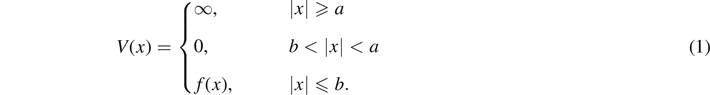
We will assume that f(x) ⩽ 0 for |x| ⩽ b and to support bound states we need f(x) < 0 for some values of x in this domain. An example of one such potential energy function is illustrated in figure 1.

Figure 1. Example potential energy function for the type of system studied. The potential energy may be non-zero (and must be negative in at least some places) for −b < x < b, but V(x) = 0 for b < |x| < a. Hard walls are placed at x = ±a.
Download figure:
Standard image High-resolution imageThe ratio of the width of the quantum well to the width of the ISW is given by r = b/a. In this paper we will show how the ZEC can be used to investigate changes in the number of bound states as r changes from 0 to 1. When r → 0 the hard walls of the ISW go to x = ±∞ and the system becomes an isolated quantum well. When r → 1 the walls of the ISW approach the edges of the quantum well at x = ±b. Note that r cannot be greater than 1 since that would make the ISW smaller than the quantum well it is supposed to contain. To ensure that the walls of the ISW approach both sides of the quantum well equally, we only consider quantum wells that are symmetric about x = 0, so f(x) is an even function. In addition, we will only consider simple wells in which the number of bound states depends only on the value of r and one other dimensionless parameter β, where β is some function of the system parameters.
For systems of this type, the ZEC is an equation relating β and r. This equation can be found analytically and the solutions to the equation form a series of curves in the (r, β) parameter space. Note that since we are finding the parameter values for a potential well that produce a given energy eigenvalue (E = 0), this approach can be viewed as an example of an inverse problem in quantum mechanics [12]. Using a plot of the ZEC curves, one can determine the maximum change in the number of bound states caused by introducing external boundaries by simply counting the number of curves that are crossed as r is changed from 0 to 1 for any β.
Because the functional form of the zero-energy eigenstate wave functions is so simple, the ZEC is mathematically simpler than the energy eigenvalue equation for the bound states, which makes this approach particularly accessible to undergraduate students. The specific quantum wells we examine are the finite square well, the triangular well (shown in figure 1), and two to five Dirac delta wells. In all of these cases the number of bound states can decrease as r is changed from 0 to 1, but the number never changes by more than two.
2. Finite square well
We will first examine a finite square well (FSW) because students are likely to encounter that system in an undergraduate quantum mechanics course [1–5]. Students will likely know that the FSW has a finite number of bound states, and always has at least one bound state. We want to show that introducing external boundaries can change the number of bound states in the well. Thus, we will examine a FSW of width 2b and depth V0 centered inside an ISW of width 2a, which is equivalent to using f(x) = −V0 in (1). To demonstrate that the introduction of external boundaries can change the number of bound states we will first derive the ZEC for this system.
The one-dimensional time-independent Schrödinger equation (TISE) for a particle of mass m in a system with potential energy V(x) is

Note that the potential energy function for the system of the FSW inside an ISW is symmetric around x = 0, so we expect the solutions to the TISE to have either even or odd symmetry. It is only necessary to solve the TISE for x ⩾ 0 for each symmetry type and then the symmetry of the solution will give the values of the wave function for x < 0: ψ(−x) = ψ(x) for even symmetry, or ψ(−x) = −ψ(x) for odd symmetry.
Zero-energy eigenstates are non-trivial solutions to the TISE with E = 0. In the region 0 ⩽ x ⩽ b the zero-energy wave function must satisfy

which can be written as

where β = 2mb2 V0/ℏ2. The dimensionless parameter β represents the scaled depth of the FSW. In the region b < x ⩽ a the wave function must satisfy

Outside of the ISW, in the region x > a, ψ(x) = 0 since the particle cannot be found outside of the hard walls.
The general solution to (4) is

while the solution to (5) is

Since the wave function must go to zero at the right wall, ψ(a) = 0 and we find that B = −Aa. Therefore,

where r = b/a.
For the wave function to be properly normalized we must ensure that

because the probability for the particle to be found in the region 0 < x < a must be exactly one half due to the symmetry of the wave function. However, since we are only concerned with finding the ZEC, and perhaps with the general shape of the wave function, it is not necessary to normalize ψ(x).
The solutions with even symmetry will be those that have an extremum at x = 0, so ψ'(0) = 0 which corresponds to setting cs = 0 in (6). To find unnormalized wave functions we can let cc = b−1/2, since cc and cs have dimension of (length)−1/2. Both ψ and dψ/dx must be continuous everywhere inside the ISW. Continuity of ψ at x = b is ensured by requiring

Continuity of dψ/dx at x = b is ensured by requiring

which gives us our solution for A. Combining (10) and (11) we find

which is the ZEC for even symmetry states.
The odd symmetry solutions must go to zero at x = 0, which is equivalent to setting cc = 0 in (6). Requiring continuity of ψ and dψ/dx at x = b, and setting cs = b−1/2 to get unnormalized solutions, results in

and

Combining (13) and (14) we find

which is the ZEC for odd symmetry states.
Table 1 summarizes the results for both even and odd symmetry zero-energy eigenstates. The table shows the ZEC as well as the limits of  as r → 0 and as r → 1 for each ZEC, where βn
denotes the nth greatest value of β that satisfies a ZEC for a given r. Because of the periodicity of the trigonometric functions that appear in the ZECs, there will be an infinite number of different β values that satisfy the ZEC, and thus an infinite number of limiting values as r → 0 or 1. However, the limiting values are always integer or half-integer multiples of π. The limit r → 0 turns the system into an isolated finite square well of width 2b and depth V0, and the ZEC in this limit gives the values of β (and thus V0) for which the well acquires a new bound state as β increases. The limit r → 1 turns the system into an ISW of width 2b but with the bottom of the well at energy −V0. In this case the ZEC gives the values of β (and thus V0) at which one of the energy levels crosses E = 0.
as r → 0 and as r → 1 for each ZEC, where βn
denotes the nth greatest value of β that satisfies a ZEC for a given r. Because of the periodicity of the trigonometric functions that appear in the ZECs, there will be an infinite number of different β values that satisfy the ZEC, and thus an infinite number of limiting values as r → 0 or 1. However, the limiting values are always integer or half-integer multiples of π. The limit r → 0 turns the system into an isolated finite square well of width 2b and depth V0, and the ZEC in this limit gives the values of β (and thus V0) for which the well acquires a new bound state as β increases. The limit r → 1 turns the system into an ISW of width 2b but with the bottom of the well at energy −V0. In this case the ZEC gives the values of β (and thus V0) at which one of the energy levels crosses E = 0.
Table 1. Zero-energy conditions and limiting values of  for a finite square well centered inside an infinite square well, where β is the scaled depth of the finite square well and r is the ratio of the width of the finite square well to that of the infinite square well. Different ZEC curves are indexed by positive integers n such that βn
is the nth greatest value of β that satisfies a ZEC for a given r.
for a finite square well centered inside an infinite square well, where β is the scaled depth of the finite square well and r is the ratio of the width of the finite square well to that of the infinite square well. Different ZEC curves are indexed by positive integers n such that βn
is the nth greatest value of β that satisfies a ZEC for a given r.
| n | Symmetry | ZEC |

|

|
|---|---|---|---|---|
| Odd | Even |
| (n − 1)π/2 | nπ/2 |
| Even | Odd |
|
Figure 2 shows a plot of  versus r for the five lowest ZEC curves in this system. Note that these plots are generated implicitly since we cannot obtain an explicit solution for
  as a function of r. The thick (blue) curves are the even-symmetry ZECs given by (12) while the thin (red) curves are the odd-symmetry ZECs given by (15). The ZEC curves divide the parameter space into regions with different numbers of bound states. The number of bound states in each region is shown by an integer in figure 2. Crossing over a ZEC curve changes the number of bound states by one. It is clear from figure 2 that the number of bound states can be changed by changing either r or β, but we will focus on how the number of bound states changes when β is held constant and only r is allowed to change. Changing r corresponds to moving the hard walls of the ISW in or out.

Figure 2. Plot of the zero-curvature conditions for a finite square well centered within an infinite square well, where β is the scaled depth of the finite square well and r is the ratio of the width of the finite square well to that of the infinite square well. Thick (blue) curves are for even-symmetry states, while thin (red) curves are for odd-symmetry states. The dotted lines show the limiting values of each curve as r → 1. Integers show the number of bound states in each region.
Download figure:
Standard image High-resolution imageNote that the value of  in the limit r → 1 is exactly equal to the value of
  in the limit r → 0. Thus, each ZEC curve spans a limited range of β and there is no overlap between these different ranges. However, the union of these ranges does cover all values of β > 0. Therefore, for any value of β it is possible to change the number of bound states by one (but not more than one) by changing only r.
Although this result may seem like nothing more than a mathematical curiosity, it is possible that it could have practical consequences for quantum wells in semiconductor devices. Consider a quantum well formed by placing a 20 nm layer of GaAs between two 'thick' layers of Ga1−x
Alx
As, which can be modeled as a finite square well with b = 16 nm, V0 = 100 meV, and the mass of the particle is given by the effective mass of the electron in the GaAs layer which is m* ≈ 0.067me where me is the electron rest mass [13]. These values correspond to β ≈ 11.2 and thus  . According to figure 2 that should mean that the well supports three bound states in the limit r → 0, when the Ga1−x
Alx
As layers are 'thick.' However, if the Ga1−x
Alx
As are made thinner, the highest energy state of even symmetry could be eliminated. Using (12) we find that this bound state disappears when r ≈ 0.164 which corresponds to a width of about 41 nm for the Ga1−x
Alx
As layers. So we see that the number of bound states in a semiconductor quantum well can differ from the value for 'thick' outer layers even when the outer layers are much thicker than the inner GaAs layer.
. According to figure 2 that should mean that the well supports three bound states in the limit r → 0, when the Ga1−x
Alx
As layers are 'thick.' However, if the Ga1−x
Alx
As are made thinner, the highest energy state of even symmetry could be eliminated. Using (12) we find that this bound state disappears when r ≈ 0.164 which corresponds to a width of about 41 nm for the Ga1−x
Alx
As layers. So we see that the number of bound states in a semiconductor quantum well can differ from the value for 'thick' outer layers even when the outer layers are much thicker than the inner GaAs layer.
It is instructive to examine the (unnormalized) wave functions for the zero-energy eigenstates in this system. Figure 3 shows plots of the zero-energy eigenstates corresponding to β4 and β5 with r = 2/3. Similar plots are shown in reference [10]. Each wave function is sinusoidal inside the FSW (|x| < b) but linear in the region that is outside the FSW but inside the ISW (b < |x| < a). The wave functions go to zero at x = ±a, but otherwise both ψ and dψ/dx are continuous. It is clear that ψ4 has odd symmetry while ψ5 has even symmetry, illustrating the general pattern that odd-n states have even symmetry while even-n states have odd symmetry. Each wave function also has a number of nodes equal to n − 1, which is a pattern also observed in bound states of quantum wells [14].

Figure 3. Wave functions for the β4 and β5 zero-energy eigenstates in the system of a finite square well inside an ISW with r = b/a = 2/3. The walls of the ISW are at x = ±a and the edges of the FSW are at x = ±b.
Download figure:
Standard image High-resolution image3. Triangular well
We have shown that external boundaries can change the number of bound states in a finite square well, but now we want to investigate how this phenomenon depends on the shape of the quantum well. Here we will consider a quantum well that students are less likely to encounter in an undergraduate course, although it is discussed in some textbooks: the triangular well [15]. We will derive the ZEC for a symmetric triangular well of width 2b and depth V0 embedded within an ISW of width 2a, which corresponds to using

in (1). The potential energy function is depicted in figure 1. The total potential energy is again symmetric about x = 0 so solutions to the TISE must have even or odd symmetry. The TISE can be solved for x ⩾ 0 for each symmetry type while for x < 0 the symmetry of the solution will give the appropriate values.
As in the FSW case, in the region b < x < a the TISE for a zero-energy eigenstate reduces to (5). However, in the region 0 < x < b the TISE for the zero-energy eigenstate is

which can be written as

where β = 2mb2 V0/ℏ2 is the scaled well depth as before.
Introducing the dimensionless coordinate

we can rewrite (18) as

The general solution to (20) is

where Ai and Bi are the Airy functions of the first and second kind, respectively [16]. The solution can be written in terms of the original position variable x as

for 0 < x < b. For b < x < a where V(x) = 0 the solution is given by (8), which satisfies the condition ψII(a) = 0. The wave function can be normalized using (9), but as before we will omit this step since it is not required for finding the ZEC or the shape of the wave functions.
The solutions with even symmetry must have ψ'(0) = 0. Using (22) this condition is satisfied if

where Ai' and Bi' are the derivatives of the Airy functions. To find unnormalized wave functions it is sufficient to set cA = b−1/2. Requiring that ψ be continuous at x = b gives

Requiring that dψ/dx be continuous at x = b gives

Combining (24) and (25) and solving for r gives

which is the ZEC for even-symmetry states.
The solutions with odd symmetry must have ψ(0) = 0. Using (22) this condition is satisfied if

and again unnormalized solutions can be found using cA = b−1/2. Continuity of ψ at x = b gives

while continuity of dψ/dx at x = b gives

Combining (28) and (29) and solving for r gives

which is the ZEC for odd-symmetry states.
Figure 4 shows a plot of ![$\sqrt[3]{\beta }$](https://content.cld.iop.org/journals/0143-0807/43/3/035407/revision2/ejpac60aaieqn12.gif) versus r for the five lowest ZEC curves (β1 to β5) for the triangular well. The plots are generated implicitly since we cannot obtain an explicit solution for
versus r for the five lowest ZEC curves (β1 to β5) for the triangular well. The plots are generated implicitly since we cannot obtain an explicit solution for ![$\sqrt[3]{\beta }$](https://content.cld.iop.org/journals/0143-0807/43/3/035407/revision2/ejpac60aaieqn13.gif) as a function of r. The thick (blue) curves are the even-symmetry ZECs given by (26) while the thin (red) curves are the odd-symmetry ZECs given by (30). Again, we see that the ZEC curves divide the parameter space into regions with different numbers of bound states, as indicated in figure 4.
as a function of r. The thick (blue) curves are the even-symmetry ZECs given by (26) while the thin (red) curves are the odd-symmetry ZECs given by (30). Again, we see that the ZEC curves divide the parameter space into regions with different numbers of bound states, as indicated in figure 4.

Figure 4. Plot of the zero-energy conditions for a triangular well centered within an ISW, where β is the scaled depth of the triangular well and r is the ratio of the width of the triangular well to that of the ISW. Thick (blue) curves are for even-symmetry states, while thin (red) curves are for odd-symmetry states. The dotted lines show the limiting values of each curve as r → 1. Integers show the number of bound states in each region.
Download figure:
Standard image High-resolution imageFor the triangular well each ZEC curve covers a limited range of β values, as was the case for the FSW. However, in this case the union of these ranges does not cover all values of β > 0. For some values of β it is possible to change the number of bound states by one (but not more than one) by changing only r, but for other values of β changing only r cannot produce any change in the number of bound states. For example, if ![$\sqrt[3]{\beta }$](https://content.cld.iop.org/journals/0143-0807/43/3/035407/revision2/ejpac60aaieqn14.gif) is between about 1.99 and 2.67 (the limits of
is between about 1.99 and 2.67 (the limits of ![$\sqrt[3]{{\beta }_{2}}$](https://content.cld.iop.org/journals/0143-0807/43/3/035407/revision2/ejpac60aaieqn15.gif) as r → 0 and as r → 1, respectively), the number of bound states can be changed between 1 and 2 by moving the ISW walls. However, if
as r → 0 and as r → 1, respectively), the number of bound states can be changed between 1 and 2 by moving the ISW walls. However, if ![$\sqrt[3]{\beta }$](https://content.cld.iop.org/journals/0143-0807/43/3/035407/revision2/ejpac60aaieqn16.gif) is between about 2.67 and 2.95 (the limit of
is between about 2.67 and 2.95 (the limit of ![$\sqrt[3]{{\beta }_{3}}$](https://content.cld.iop.org/journals/0143-0807/43/3/035407/revision2/ejpac60aaieqn17.gif) as r → 0) then the system has two bound states regardless of where the walls of the ISW are placed. Although the ZEC curves get closer together at higher values of β, this general pattern continues: for some ranges of β the number of bound states can change by one when changing only r while for other ranges the number of bound states cannot be changed by changing only r. Thus, the introduction of external boundaries seems to have less effect on the number of bound states in the triangular well than in the finite square well.
as r → 0) then the system has two bound states regardless of where the walls of the ISW are placed. Although the ZEC curves get closer together at higher values of β, this general pattern continues: for some ranges of β the number of bound states can change by one when changing only r while for other ranges the number of bound states cannot be changed by changing only r. Thus, the introduction of external boundaries seems to have less effect on the number of bound states in the triangular well than in the finite square well.
Figure 5 shows plots of the zero-energy eigenstates corresponding to β4 and β5 for this system with r = 2/3. Each wave function is oscillatory inside the triangular well (|x| < b), with the amplitude increasing toward the outer edges of the well where a classical particle would move more slowly (and thus have a higher probability of being found). Outside the triangular well, but inside the ISW, the wave functions are linear. The wave functions go to zero at x = ±a, but otherwise both ψ and dψ/dx are continuous. As in the cases examined previously, odd-n states have even symmetry and even-n states have odd symmetry, and each wave function has n − 1 nodes.
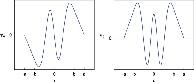
Figure 5. Wave functions for the β4 and β5 zero-energy eigenstates in the system of a triangular well inside an ISW with r = b/a = 2/3. The walls of the ISW are at x = ±a and the edges of the triangular well are at x = ±b.
Download figure:
Standard image High-resolution image4. Delta wells
External boundaries seem to have less effect on the number of bound states in the triangular well than in the finite square well, which suggests that changing the shape of the well so that it is deeper in the center than on the sides reduces the impact of external barriers on the number of bound states. Next we will consider a case in which quantum well is especially deep near the sides of the well at |x| = b. For this purpose we will examine a quantum well composed of two or more Dirac delta function wells, a quantum well that students may encounter in an undergraduate course but that has also proved useful for modeling a variety of short-range interactions [17–19]. The full system will consist of N identical delta wells, equally spaced between x = −b and x = b, inside an ISW of width 2a. This amounts to using

in (1), where V0 is a characteristic energy that controls the strength of the particle's interaction with the delta well, N is the number of delta wells, and

gives the location of the ith delta well.
The delta wells divide the interior of the ISW into N + 1 intervals. The wave function within each interval is denoted ψj such that ψ1 is the wave function on −a ⩽ x < x1, ψ2 on x1 ⩽ x < x2, etc. Within each of these regions the potential energy is zero and the TISE for a zero-energy eigenstate is given by (5), so the solution will be of the form

Thus, the wave function for the zero-energy state in this system is piecewise linear, so it may be referred to as a zero-curvature state [7, 9, 11]. Proper normalization of the wave function is achieved by requiring

Since we are only concerned to find the ZEC for the system and show the shape of the wave functions it is not necessary to impose this normalization condition.
The wave function must go to zero at the left wall of the ISW, so

and therefore B1 = A1 a. Since we are content to find unnormalized eigenfunctions, we can simply set A1 = b−3/2 and then B1 = b−3/2 a = b−1/2 r−1.
To determine the values of Aj and Bj in the other regions we first require that the wave function be continuous at the location of each delta well, so

Because the delta wells create an infinite discontinuity in the potential energy at x = xi , the slope dψ/dx may be discontinuous at x = xi [17]. However, the discontinuity in slope must satisfy

where β = 2mb2 V0/ℏ2 is a dimensionless parameter that characterizes the strength of the delta well interaction. Combining (33) with (37) we find

The system of equations given by (36) and (38) can be solved for Ai+1 and Bi+1. We write the solution in matrix form:

where

is known as a transfer matrix [20].
Combining (39) with our results for A1 and B1 we find

If the wave function is to be a valid zero-energy eigenstate then it must go to zero at the right wall of the ISW, so

We can rewrite this condition using (41) as

which is the ZEC for the system with a given set of parameter values (N, β, and r).
We will not consider the case of a single delta well (N = 1) in detail, because such a well has zero width and therefore r = b/a = 0 regardless of the value of a. However, we do note that an ISW with a single delta well placed at the center does admit a zero-energy eigenstate [7, 9, 11, 18]. The ZEC for this system is

where in this case b is just an arbitrary length unit since it cannot represent the half-width of the quantum well. We see that lima→∞ β = 0 and lima→0 β = ∞, which indicates that this system supports one bound state for any β > 0 in the limit a → ∞ (an isolated delta well) and supports no bound states for any β in the limit a → 0. Thus, imposing external boundaries for an single delta well changes the number of bound states by at most one, just as we saw for the finite square and triangular wells.
The results are more interesting for N ⩾ 2. We will show results for N = 2, 3, 4, and 5. Recall that the wells are equally spaced from x1 = −b to xN = b so that the collection of wells has a width 2b and r = b/a is the ratio of the width spanned by the delta wells to the width of the ISW. For N = 2 we will have delta wells at x = −b and b. For N = 3 there are wells at x = −b, 0, and b. For N = 4 the wells are located at x = −b, −b/3, b/3, and b. Finally, for N = 5 the wells are at x = −b, −b/2, 0, b/2, and b. These example are sufficient to show the basic pattern, so we will not show results for larger values of N.
Because the potential energy function is symmetric about x = 0 we expect the zero-energy eigenstate wave functions to have even or odd symmetry. Wave functions with odd symmetry must go to zero at x = 0, while those with even symmetry do not. Although we could have derived separate ZECs for each symmetry type, as we did earlier with the ISW and the triangular well, the ZEC in (43) includes both symmetry types. We find that the left side of (43) is a polynomial of degree N in β, so the equation can have up to N real-valued solutions. This polynomial can always be factored into two polynomials of lesser degree: one that gives values of β for the even-symmetry zero-energy states and another that gives β values for the odd-symmetry states. For example, the polynomial for N = 4 factors into the product of two quadratic polynomials, one for each symmetry type.
We can analytically solve the resulting polynomial equations for β in terms of r. The ZEC equations for N = 2, 3, and 4 are shown in the third column of table 2. As before we number the values of β that satisfy the ZEC from least to greatest, with β1 being least. The odd-numbered values of β correspond to states with even symmetry, while the even-numbered values correspond to states with odd symmetry. The N = 5 polynomial factors into a cubic and a quadratic. The solutions from the cubic polynomial are much more complicated, so the ZEC equations for this case are shown only in the supplementary materials (https://stacks.iop.org/EJP/43/035407/mmedia).
Table 2. Zero-energy conditions and limiting values of β for a system of N identical, equally-spaced delta wells centered inside an ISW, where β is the scaled interaction strength and r = b/a is the ratio of the width spanned by the delta wells to the width of the ISW. Different ZEC curves are indexed by positive integers n such that βn is the nth greatest value of β that satisfies the ZEC for a given N and r.
| N | Symmetry | ZEC | limr→0 βn | limr→1 βn |
|---|---|---|---|---|
| 2 | Even |

| 0 | ∞ |
| Odd |

| 1 | ∞ | |
| 3 | Even |
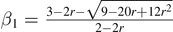
| 0 | 2 |
| Odd |

| 1 | ∞ | |
| Even |
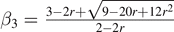
| 3 | ∞ | |
| 4 | Even |
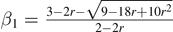
| 0 | 3/2 |
| Odd |

|

| 9/2 | |
| Even |
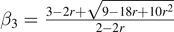
| 3 | ∞ | |
| Odd |
|

| ∞ |
Table 2 also displays the values of β for each ZEC in the limits r → 0 and r → 1. Plots of the ZEC curves for N = 2, 3, 4, and 5 are shown in figure 6. We see that in each case the (r, β) parameter space is divided into N + 1 regions separated by the ZEC curves. The region below and right of the β1 curve does not support a bound state. Moving upward or to the left in the parameter space may result in crossing a ZEC curve. Each time a ZEC curve is crossed in this direction the number of bound states in the system increases by one. The region above and left of the βN curve supports N bound states.

Figure 6. Plots of the zero-energy conditions for N = 2, 3, 4, and 5 evenly-spaced delta wells centered within an infinite square well, where β is the scaled interaction strength and r = b/a is the ratio of the width spanned by the delta wells to the width of the infinite square well. Thick (blue) curves are for even-symmetry states, while thin (red) curves are for odd-symmetry states. The dotted lines show the limiting values of each curve as r → 1. Integers show the number of bound states in each region.
Download figure:
Standard image High-resolution imageIn general, by changing the parameters of the system we can change the number of bound states to any value between 0 and N. However, if we leave β fixed and change only r, then the change in the number of bound states is more restricted. Careful examination of the limiting values of β as r → 0 and as r → 1 shows that although each ZEC curve spans a limited range of β values, some of these ranges overlap. As a result, for some values of β it is possible to cross two ZEC curves by changing only r. Moreover, the union of the β ranges spanned by the ZEC curves covers all values of β > 0, so for any value of β it is possible to change the number of bound states by at least one by changing only r. For example, when N = 3 we can change the number of bound states by two just by moving the ISW walls as long as 1 < β < 2 or β > 3. However, for β < 1 or 2 < β < 3 we can change the number of bound states by at most one when moving the ISW walls.
Note that in the limit r → 0 there is always at least one bound state for β > 0 and for higher values of β the number of bound states can increase up to N. This is exactly what is expected for a collection of isolated delta wells. In the limit r → 1, on the other hand, there may be no bound states for low values of β > 0 and the maximum number of bound states is N − 2. In this limit the walls of the ISW approach the two outermost delta wells and when r = 1 those two delta wells are absorbed into the walls of the ISW. Therefore, the results for N wells in the limit r → 1 correspond to a situation with N − 2 wells.
For example, for N = 4 in the limit r → 1 the delta wells at x = ±b are absorbed and the resulting system has two delta wells at x = ±b/3 and ISW walls at x = ±b. This corresponds to the N = 2 system with r = 1/3 but with a different value of b: b' = b/3. To keep the strength of the delta wells the same in (31) we must also use  . Together b' and
  lead to β' = β/3, so the (finite) β values for the ZEC with N = 4 and r = 1 can be divided by three to get the β values for N = 2 with r = 1/3. Similarly, the finite β values for N = 5 with r = 1 can be divided by two to get the values for N = 3 with r = 1/2. These relations can be verified using the ZEC equations in table 2 or the plots in figure 6.
Obtaining analytical solutions for the ZEC becomes more difficult as N increases since larger values of N result in higher degree polynomials in the ZEC. However, we expect that the pattern established above will continue to hold for N > 5: for some values of β the number of bound states can be changed by at most two when changing only r, while for other β values the change will be at most one. The top two curves will always have vertical asymptotes at r = 1 while the remaining curves will approach finite values at r = 1 that correspond to some set of values for a system with two fewer delta wells.
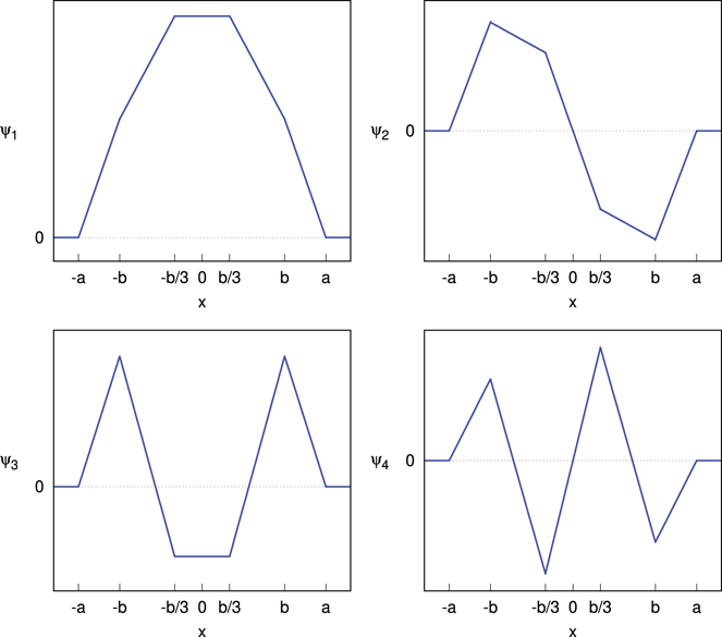
Note that if the zero-energy eigenstate does exist, then the coefficients Aj and Bj for the (unnormalized) wave function given in (33) can be computed through repeated application of (39) starting with A1 = b−3/2 and B1 = b−1/2 r−1. Figure 7 shows plots of the wave functions for N = 4 with r = 2/3, where ψn corresponds to the zero-energy eigenstate with β = βn . It is clear that the wave functions are linear and continuous everywhere but may have discontinuities in dψ/dx at the locations of the ISW walls and the delta wells. The wave functions display either even or odd symmetry, with odd-numbered states having even symmetry and even-numbered states having odd symmetry as noted earlier. The number of nodes for ψn (x) is equal to n − 1 as expected.
Figure 7. Wave functions for the zero-energy eigenstates in the system of N = 4 evenly-spaced delta wells centered inside an ISW with r = b/a = 2/3. The delta wells are located at x = ±b and ±b/3, while the ISW walls are at x = ±a.
Download figure:
Standard image High-resolution image
The wave functions shown in figure 7 display some similarity to the sinusoidal standing wave solutions for the ISW without delta wells. Indeed, as β → 0 each of these states will change into the corresponding ISW eigenstate [21].
The general pattern shown for N = 4 is maintained for other values of N. If the states are numbered in terms of increasing values of β then ψ1 will have even symmetry and no nodes, ψ2 will have odd symmetry and one node, ψ3 even symmetry and two nodes, and so on. One notable difference that occurs for odd values of N is that odd symmetry states will not have a discontinuity in dψ/dx at x = 0, even though there is a delta well at that location. This situation occurs because the wave function has a node at x = 0 and thus the delta well at x = 0 can have no effect on odd-symmetry eigenstates, as indicated by (37).
5. Conclusion
We have shown that the number of bound states in a one-dimensional quantum well depends on conditions outside of the well. In particular, we have shown that imposing hard walls outside of a quantum well can change the number of bound states in the well. We examined several different quantum wells: a finite square well, a triangular well, and two to five evenly-spaced, identical Dirac delta wells. In each case the quantum well was centered inside an ISW. We found that in some cases the number of bound states in the quantum well could be decreased by moving the walls of the ISW inward, or increased by moving the walls of the ISW outward. For the finite square well the number of bound states changed by at most one when moving the ISW walls, regardless of the scaled depth of the well. For the triangle well the number of bound states changed by at most one when moving the ISW walls for some values of the scaled well depth, while for other scaled depths the number of bound states could not be changed in this way. Finally, for multiple delta wells the number of bound states changed by at most one when moving the ISW walls for certain values of the scaled interaction strength, while for other values of scaled interaction strength the number of bound states changed by at most two.
Our results suggest that, although imposing boundaries outside of a one-dimensional quantum well can alter the number of bound states in the well, there are limits on how much the number of bound states can be changed. Specifically, in systems composed of multiple delta wells the limit on the change in the number of bound states appears to be two, while for other one-dimensional quantum wells the limit seems to be one. More evidence for this conjecture (or a counterexample to disprove the conjecture) could be obtained by examining quantum wells with other shapes, including asymmetric wells and systems of delta wells that are not identical and not evenly spaced.
In addition to the results discussed above, our work illustrates that zero-energy eigenstates can serve as a useful tool for studying how the number of bound states in a quantum system depends on the system parameters. Although zero-energy eigenstates have pedagogical value and may play an important role in wave packet dynamics, scattering [10, 22], or the creation of designer wave functions [7, 9], we are not aware of other studies that have used the condition for the existence of zero-energy eigenstates as a means of investigating the number of bound states in a quantum well. Because the zero-energy states have a simpler mathematical form than the bound states (i.e. they are linear rather than exponential in the regions where V(x) = 0), the ZEC may provide a way for students to investigate the number of bound states in a system that is more accessible than the usual energy eigenvalue equation for the bound states.
Acknowledgments
The authors would like to thank the Berry College LifeWorks program and the Berry College Honors Program for their support of this work.