

Abstract
High-temperature superconductors (HTS) can be superconducting in liquid nitrogen (77 K) at atmospheric pressure, which holds immense promises for our future such as nuclear fusion, compact medical devices and efficient power applications. In a power system, high short-circuit currents can exceed the operational current by more than ten times, putting many parts of the system at risk. Superconducting fault current limiters (SFCLs) can limit the prospective fault current without disconnecting the power system, and are thus becoming increasingly attractive for future grids. With a growing interest in modeling and commercializing SFCL, the question of how to teach and to explain their operation to students has arisen. In order to help students visualize the potential use and benefits of an SFCL, we created an executable and a web application using COMSOL Multiphysics. This executable allows students to investigate the electro-thermal response of a resistive SFCL. The executable solves a 1D electro-thermal model of the SFCL under AC fault conditions, evaluating important figures of merit such as the limited current, the prospective current and the maximum temperature reached within the tape. Finally, the geometrical parameters as well as the superconducting properties of the device can be modified. The importance of the amount of silver stabilizer necessary to protect the device from over-heating occurring during a fault current can be investigated. In addition, the effects of having a sharp nonlinear transition from the superconducting to the normal state (intrinsic property of the superconductor) to obtain a current limitation can be explored. The executable allows the users to learn about the benefits of superconductors in real-life applications, without the prerequisite of extensive modeling or experimental setup. The executable can be downloaded from the HTS modeling website and run on the most commonly used operating systems.
Export citation and abstract BibTeX RIS

Original content from this work may be used under the terms of the Creative Commons Attribution 4.0 licence. Any further distribution of this work must maintain attribution to the author(s) and the title of the work, journal citation and DOI.
1. Introduction
Given the ever increasing role of electricity in our society, protecting electric grids from faults and surges has become of paramount importance. Among the different categories of faults in a power distribution grid, animal-caused faults account for 10%–20% of the electrical disruption events—especially squirrels chewing the wire's insulation of overhead lines [3] and creating an arc with their own body. A short-circuit can also happen when a tree falls over an overhead line because of weather-related reasons (wind or snow). When this happens, the tree links the line to the ground and an electric arc appears. In order to prevent faults, different technologies have been developed: these include explosive Is-limiters, high-voltage fuses and air-core reactors. These technologies, while effective, present important limitations, for example added circuit impedance during normal operation, limited scalability, and high maintenance efforts [4]. The disruptive technology offered by superconductivity allows overcoming these limitations 3 . Superconducting fault current limiters (SFCLs) are devices that are essentially 'transparent' during normal operation (with no or very limited energy dissipation) and that present an extremely rapid and large increase of their resistance during a fault. In resistive SFCL, this behavior comes from the intrinsic physical properties of the superconducting material, i.e. an extremely non-linear dependence of the resistance on the current flowing through the device (figure 1) 4 . During normal operation, the superconductor operates in the zero-resistivity region represented in figure 1(a), where it has no (in direct current regime) or very low (in alternating current regime) losses 5 . During a fault, the resistivity of the superconductor increases rapidly to extremely high values, i.e. 100 μΩ cm in the normal-state (figure 1(a)): this increase of the material's resistivity can be used to limit the current flowing in the electric circuit, thus protecting the load. Figure 1(b) represents what occurs to the current flowing in the grid during a fault if a current limiter is present (continuous blue line) or not (red dashed line). Without a fault current limiter (FCL), the large current oscillations resulting from the fault put the grid equipment at risk. The ultimate effect of a non-limited fault is an economic damage for both the operator and the customer. The optimal location in the grid of these devices depends on several factors like fault current reduction, grid reliability, FCL cost reduction and recovery time optimization. Several optimal placement techniques have been reported in the literature [5, 6, 8, 9], some of which are capable of handling complexities such as uncertainties in the fault locations and unpredictable variations of the power system conditions. High-temperature superconductors (HTS), with critical temperatures well above the boiling temperature of liquid nitrogen at atmospheric pressure (77 K), are particularly indicated for SFCL applications: compared to classical low-temperature superconductors, they have lower refrigeration costs and increased heat capacity. Currently, the most promising HTS are manufactured in the forms of multi-layer tapes, where the superconductor material is a thin film, only a few micrometers thick. Additional copper layers provide electrical and thermal stabilization. The superconducting material has the chemical formula (RE)Ba2Cu3O7, where RE indicates a rare earth element. They are often indicated as REBCO coated conductors and their typical structure is shown in figure 2.
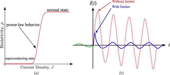
Figure 1. (a) Non-linear dependence of the superconductor's resistivity on the current density and (b) schematic representation of what occurs to the current flowing in the grid during a fault if a current limiter is present or not.
Download figure:
Standard image High-resolution image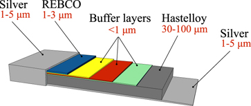
Figure 2. Typical structure of a REBCO commercial tape (representation not to scale).
Download figure:
Standard image High-resolution imageThe performance of coated conductors in SFCL dramatically depends on their structure (e.g. the thickness of the different layers), on the physical properties of the superconductor material, and on the cooling conditions. Researchers around the world are trying to optimize REBCO coated conductors for SFCL applications [10–13].
The aim of this work is to introduce the readers to the use of REBCO coated conductors for resistive SFCL application, with particular focus on the impact of the tape's structure and physical parameters on the current limiting behavior. A finite-element model was developed for this purpose, simulating the electro-thermal characteristic of the tape in fault-current limiting applications. The used commercial software was COMSOL Multiphysics, and the application was distributed as a COMSOL application, as an executable [1], and as a web application within the project leArning sUpeRcOnductivity thRough Apps (AURORA) [2].
With a simulation application, complex concepts can be incorporated behind a user-friendly interface, so that users do not have to deal with unnecessary jargon. In addition, this type of applications enables an easy access to simulation tools that can generate interest in students and provide values to companies.
2. Superconducting fault current limiters
In resistive SFCL, after transition, the superconducting tape needs to absorb and spread the energy during the limitation phase. Ideally, the transition from the superconducting to the normal state occurs uniformly along the tape's length. The energy balance can be written as follows:

where the dissipated energy (left-hand side) is either absorbed by the wire (right-hand side, first term) or exchanged with the cryogenic bath (right-hand side, second term). In equation (1), Ltape is the tape's length, tlim is the time duration of the limitation, E(I, T) is the electric field (which depends on the current I and on the temperature T), m is the tape's mass, Cp is the tape's heat capacity, and T0 is the starting operating temperature 6 .
In the analysis presented in equation (1), we introduce a few simplifications. If the quench is sufficiently fast, the energy exchange with the bath is low: we are close to adiabatic conditions and the term Qbath is negligible. In addition, for a clear fault, i.e. I ≫ Ic, the REBCO material switches instantaneously to very high resistivity; therefore E does not depend on I anymore, the current flows only in the stabilizer and in the substrate. In order to avoid permanent damage to the superconducting tape, the final temperature T(tlim) has to be under a certain limit, generally between 400 K and 450 K for coated conductors. Then, for a given limitation time, the main structural parameters around which the construction of the device can be adjusted are the mass of the conductor, which can be increased by making the tape thicker and/or longer, and the amount of stabilizer, which controls the resistance of the tape in normal state. The generated heat must be sufficiently uniform and the conductor's length kept within reasonable limits for economic reasons.
The electric field E is a parameter characterizing the device: 50 V m−1 is a typical value for a tape with a 100 μm-thick substrate. A higher mass per unit length obtained by using a thicker substrate or even by adding high Cp(T) material tightly thermally connected to the conductor will result in a higher electric field, up to 200 V m−1. Higher electric fields can be obtained by using sapphire-based substrates [15]: their very high thermal conductivity would allow a millimeter-thick substrate without significant thermal gradient on the cross section.
In resistive SFCL, the superconducting tape needs to be sufficiently long in order to absorb and spread the energy during limitation. In order to limit the size of the device, the tape is wound in the form of pancake coils, with a bifilar design (figure 3(a)), where the current of adjacent turns flows in opposite directions. This greatly reduces the coil's impedance and, thanks to the suppression of the magnetic field component perpendicular to the flat face of the tape, the AC losses as well [16]. A picture of the bifilar coil module used in the Ensystrob project [17] is shown in figure 3(b).

Figure 3. Bifilar coils for SFCL application: schematic illustration and picture of the module used in the Ensystrob project [17].
Download figure:
Standard image High-resolution image3. COMSOL model of HTS wire for fault current limiter applications
In this section we describe the model implemented in the commercial software COMSOL Multiphysics [18]. A similar model was developed by the authors in [19].
3.1. Equivalent 1-D thermal and electrical model of an SFCL
The heat equation was solved on a 1-D domain and it was coupled with an electric circuit model, simulating the current sharing between the layers of the tape. A 1-D thermal assumption entails that the electrical and thermal properties of the tapes are uniform along the width and length of the tape (temperature distribution across the thickness of the tape). In figure 4, we represented the equivalent electrical model of the SFCL. The equivalent model of the SFCL is a set of resistors in parallel, representing the various layers of the tape (silver stabilizer, Hastelloy and REBCO). We do not take into account the buffer layer and the interface resistance between REBCO and silver layer. Each resistor (layer) Ri (Ii , Ti ) is defined by the electrical resistivity ρel,i (Ii , Ti ), the length of the tape Ltape, the thickness of the single layer hi and the width of the tape wtape. The subscript i identifies the layer of the tape (i.e. silver, REBCO, etc). The heat equation is coupled with the equivalent circuit model of the SFCL through the heat source. In each 1-D domain, schematically represented in figure 4, the heat equation is solved as follows:
On the left side of the one-dimensional heat equation we have the mass density ρmass,i
(Ti
), the specific heat capacity Cp,i
(Ti
) and the thermal conductivity ki
(Ti
). On the right side of equation, there are the heat source and the cooling terms. The cooling term accounts for the heat exchange with the liquid nitrogen. This is done by applying a boundary condition only on the top and the bottom layers of the tape (silver surfaces), indicated by ∂Ω. In equation (2), the heat transfer coefficient hLN2(Ti
− T0) is a function of the temperature [20]. For better readability, the temperature dependence of hLN2(Ti
− T0) is omitted and the transfer coefficient is simply written as hLN2. The temperature dependence of all the thermal and electrical material properties is taken into account. Finally, the heat source comes from the joule heating effect  , where the volume of each layer is noted as Ωi
= wtape ⋅ Ltape ⋅ hi
.
, where the volume of each layer is noted as Ωi
= wtape ⋅ Ltape ⋅ hi
.
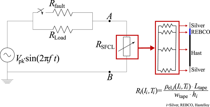
Figure 4. Schematic circuit representing the electric circuit model, and representation of the REBCO tape implemented in COMSOL Multiphysics.
Download figure:
Standard image High-resolution imageFor modeling the REBCO resistivity, we consider the widely used power-law model with a temperature-dependent critical current Ic(T). The power-law model reads as follows:

where Σ is the cross section of the REBCO layer, Ec = 1 μV cm−1 is the electric field criterion and n is the constant power-law exponent, and Ic(T) reads as follows:

In order to obtain a total resistivity that better reproduces the electrical behavior of REBCO over a wide current and temperature range, the normal state resistivity ρNS(T) of REBCO is added in parallel to the power-law [21]

Finally, the temperature dependence of the normal-state resistivity of REBCO is modeled with a linear relationship [22], i.e.:

where  and α = 0.47 μΩ cm K−1 [23].
The complete circuit model used to simulate AC fault current limitation is presented in figure 4. A sinusoidal voltage signal is imposed on the circuit, while a load resistor RLoad draws the nominal current from the source. A switch in parallel to the load resistor, when closed, simulates the fault occurring at a given time and draws the fault current through a resistor Rfault. In the simulations, Vpeak can be changed and f = 50 Hz is fixed. The switch operates at t = 20 ms and the short-circuit is cleared after two periods of the sinusoidal voltage source, i.e. t = 60 ms. Finally, the prospective current is calculated as Ifault = Vpeak/Rfault.
3.2. Heat equation in 1D to estimate the cooling temperature profile
Another interesting aspect is the temperature cooling profile of the tape. Once the superconducting tape has recovered from the fault, the nominal operation of the grid must be re-established. This means that the SFCL must also be invisible to the grid (negligible impedance) and thus in the superconducting state. This condition implies that the temperature of the REBCO layer must be below its critical temperature Tc, which is around 92 K [24].
The complex non-linear heat transfer coefficient of the liquid nitrogen does not allow to estimate the cooling-temperature profile of the SFCL analytically, and thus, its recovery time. As a consequence, these quantities are estimated with numerical methods.
The time-scale at which the fault occurs (tens of ms) is very different from that of cooling, which is typically around hundreds of ms or s. The numerical solution of phenomena occurring at very different time-scales can lead to long computational times. This is undesired, especially when the user expects the simulation to run in a few minutes, as in the case of a student during a lecture. To address this issue, one can note that during the cooling of the tape the only physics involved is the heat transfer between layers and liquid nitrogen. As a consequence, we can neglect the circuital part and study the temperature profile of the tape with a second model. The second model uses the temperature profile of the tape at the end of the first simulation as initial condition, and the initial time of the second model is the final one of the first modelt0 = tfin. As a consequence we have:

The second model solves the heat equation on the same domains, but for a longer time (i.e. 2 s) and with a larger time step. This ensures the simulation of a time sufficiently long to observe the temperature cooling profile while having a short computational time.
The computing time of the first model (fault over 100 ms) ranges from 30 s to 40 s per run, while the computing time of the second model (tape cooling from 100 ms to 2 s) ranges from 6 s to 10 s per run. Once the simulation is run, the solver is concatenated and the overall simulation takes from 35 s to 60 s run. These computing times were obtained by running the executable on an Intel(R) Core(TM) i5-7Y57 CPU @ 1.30 GHz).
Since the main design criteria are to avoid burning the tape, we need to know whether this happened after the fault. At the end of the simulation, a dialogue box informs about the status of the tape. Specifically, the box informs if the tape reached more than 450 K and if, after 2 s 7 , the tape recovered, and its temperature is below 92 K. The maximum temperature displayed in the box is obtained by calculating the average temperature profile on the 1-D REBCO domain and selecting the maximum value of this curve.
3.3. User interface and parameter calibration
In figure 5 we present the user interface. In the upper part (black-dashed box), we have the dashboard where we can find the functional buttons of the executable. Besides running the simulations ('compute') and plotting the results ('plot'), it is possible to consult a presentation describing some relevant test cases ('slide/paper') and also to export the results in form of report (.html/.doc). The parameters that can be changed and some figures of merit are indicated in figure 5.
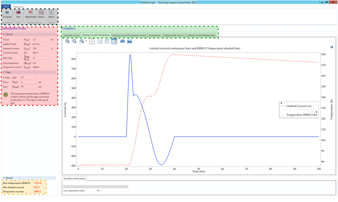
Figure 5. Screenshot of the executable. A description of the various parts is given in the text.
Download figure:
Standard image High-resolution imageIn the circuit drop-down list, the parameters that can be varied are Vpk, Inom and Ratio = RLoad/Rfault. By selecting Vpk, one fixes the applied electric field Eapp, since both the length of the tape (ltape = 200 m), as well as its width (wtape = 12 mm), are fixed by design. By choosing Inom, one selects the nominal current flowing in the circuit in normal conditions. The critical current of the tape Ic (at 77 K and self-field conditions) is fixed accordingly, and arbitrarily, as Ic = 1.2Inom. Finally, by selecting the ratio between the nominal and fault impedance, one selects the prospective current as Iprosp = Ratio ⋅ Inom. At this point the user should select the tape parameters in the tape drop-down list. The parameters that can be changed, in this case, are the n-value, the silver thickness hAg and the Hastelloy thickness hHast.
Once the parameters are set and the simulation is finished, the user can consult some figures of merit such as the maximum temperature of the REBCO, the maximum limited current, and the prospective current (yellow-dashed box). Finally, the user can browse through the plots that report the quantities calculated from the model, such as the limiting current—temperature of the REBCO, the limiting current—prospective current, and the temperature cooling profile over 2 s (green-dashed box).
4. Results
In this section we present four cases obtained by varying the parameters described above. We selected four case scenarios to highlight the importance of a sharp nonlinear transition, as well as the role played by the amount of stabilizer and Hastelloy. The parameters (referring to figures 4 and 5) are Vpk, Inom, Ratio and n0, hAg, hHast.
The user should tweak the parameters to assess how the output results change with respect to a given quantity. For instance, what happens if the n-value, which defines the strong non-linearity of the superconductor, is reduced?
4.1. Default parameters
The first case investigates the default parameter setting, namely:
- Vpk = 12 kV (Eapp = 60 V m−1)
- Inom = 500 A (Ic = 600 A)
- Ratio = 4 (Iprosp = 2000 A)
- n0 = 30
- hAg = 2 μm
- hHast = 50 μm.
As shown in figures 6(a)–(c), with these parameters the tape is safe: the temperature stays below 450 K for the entire duration of the fault, and the limited current (<1000 A) is smaller than the prospective one (2000 A).
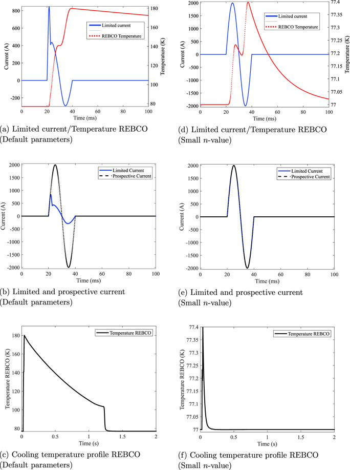
Figure 6. Simulation results using (left) the default parameters and (right) a small n-value.
Download figure:
Standard image High-resolution image4.2. Small n-value (low non-linear behavior)
In the second case all the parameters are kept as in the first case, except for the n-value. In this case the n-value is very small (i.e. n = 5) with respect to the commonly n-values of REBCO tapes (i.e. n ≈ 30 [25]). The superconductor has a smoother transition to the normal state and its behavior is closer to that of an ohmic material (n = 1).
The results (figures 6(d)–(f)) show that, for n = 5, the current flowing in the system is overlapped to the prospective current, and thus, the current is not limited (figure 6(d)). The simulated temperature profile in the REBCO predicts a very small temperature increase (ΔT ≈ 0.4 K). This means that the REBCO tape is still safe; however it is possible that other parts of the system, sensitive to overcurrents, are permanently damaged. This case highlights the crucial role played by the high non-linearity of the superconductor in making the current limitation effective.
4.3. Low impedance fault, higher applied electric field, and thin Hastelloy layer
The third case investigates a more realistic situation, where the prospective fault current can reach 10–12 times the critical current, and the applied electric field is higher. All the parameters are kept as in the first case except for Vpk = 40 kV (Eapp = 200 V m−1) and Ratio = 10 (Iprosp = 5000 A). The results in figures 7(a)–(c) show that the limited current (<1000 A) is smaller than the prospective one (5000 A). However, the REBCO tape is burnt since the temperature goes above 450 K. A possible solution is to add mass to the tape. This can be done by increasing the thickness of the Hastelloy layer.

Figure 7. Simulation results for a high prospective current fault with a (left) thin and (right) thick Hastelloy layer.
Download figure:
Standard image High-resolution image
4.4. Low impedance fault, higher applied electric field, and thick Hastelloy layer
In the last case scenario we keep the same circuit parameters of the previous case, but we increase the thickness of the Hastelloy layer to 100 μm. The results are presented in figures 7(d)–(f). The electrical quantities (voltage and current) are the same, while the simulated temperature in the REBCO is substantially decreased and is below 450 K.
5. Conclusion
In this paper we presented an executable that can be used to introduce students to the benefits of using superconductors in power applications, specifically a resistive SFCL. The executable solves a 1D electro-thermal model of the SFCL under AC fault conditions. With this tool, students can learn about the influence of circuit and tape parameters on the electro-thermal behavior of an SFCL. We presented four cases to highlight the importance of a sharp nonlinear transition, as well as the role played by the amount of Hastelloy. The students however, can quickly simulate different cases since the running time is relatively short (tens of seconds). The model is developed in COMSOL Multiphysics and is deployed in various forms, including executable files (running on the most common operating systems) [1] and as web application within the project AURORA [2].
Acknowledgment
This research was supported by EPFL and the Swiss Federal Office of Energy SFOE under Grant Agreement SI/500193-02. We want to thank Ivar Kjelberg (CSEM SA) for having provided feedback and the executable App, Sven Friedel (COMSOL Switzerland) for his collaboration and EPFL for having provided an open-access server.
Supplementary data
Footnotes
- 3
- 4
Other types of SFCL exist, for example bridge-type and shielded iron core fault SFCL. In those cases, only a small part of the energy is dissipated in the superconductor itself. See [4] for details and examples. In this article we consider only resistive SFCL.
- 5
An introduction to the topic of AC losses in superconductor, which includes a numerical model implemented in an open-source finite-element program, can be found in [7].
- 6
A less ideal situation is represented by high-impedance faults, with the current I close to Ic. In such cases, the non-homogeneity of the critical current along the conductor leads to localized transitions to normal state and to the formations of the so-called hot spots. The same energy balance given by equation (1) applies locally and tlim has still to be short enough. In practice, it is quite difficult to detect the hot spots early enough to maintain tlim short and thus keep the local temperature at a safe value. A high normal zone propagation velocity is helpful to protect against hot spots [14].
- 7