

Abstract
We present and discuss a non-expensive mechanical experiment which is very suitable for a classroom demonstration of the fold catastrophe behaviour. The apparatus consists of a bar attached to a pulley, to which a hanging body is connected by means of a thread wrapped around its rim. The system may perform stable oscillations or, else, the body may continuously fall down, while the pulley executes a sequence of 360° rotations. This behaviour is analysed in connection with the shape of the potential, which is a good example of a fold catastrophe potential. For the system to perform stable oscillations, that shape reminds a clothes washboard, with local maxima and minima, a potential well known in superconducting quantum computing. We provide some hints for the instructor to explore the device in lab classes.
Export citation and abstract BibTeX RIS
1. Introduction
Quantum computing is now a promising technology, embracing Mathematics, Computer Science and Physics [1], potentially able to gradually taking over the high performance computing ecosystem, though this may certainly happen many years or even decades from now. A most significant aspect is the use of qubits based on superconductor architectures. A particular feature of qubits superconducting quantum circuits is the usage of the Josephson's junctions, which are superconductor/insulator/superconductor interfaces [2]. The theoretical explanation of the physical behaviour is described by means of a so-called tilted washboard potential [3], the name coming from its shape, with ups and downs, reminding the board where clothes used to be washed. In this article, we will explore the richness of this potential at the classical level, which, on the other hand, turns out to be a good example of a potential exhibiting a fold catastrophe.
A fold catastrophe refers to a system where a single control parameter can cause equilibria to appear or disappear [4–7]. The pertinent potential is a special case of nonlinear potentials studied in the framework of the catastrophe theory. These potentials have critical points (the bifurcation points), in which not only the first derivative but one or more higher derivatives are also zero. At the critical point(s) the behaviour of the system changes qualitatively as a consequence of small changes of control parameters. The potentials are analysed by performing the Taylor expansion around the critical point, allowing the parameters of the potential to deviate from their critical values.
A fold catastrophe involves only one parameter, a, and the expended potential can be cast in the form U(x) = x3 + ax. The bifurcation point occurs for a = 0; for a < 0 a stable and an unstable extrema exist; for a > 0 there is no stable solution.
Another physically interesting case is the cusp catastrophe corresponding to U = x4 + ax2 + bx, which for b = 0 represents the potential used to describe spontaneous symmetry breaking, well known in particle physics (e.g. Higgs mechanism) and in superconductivity (Ginzburg–Landau theory). For a > 0 a stable minimum exists at x = 0, while for a < 0 this minimum turns into a maximum and, in addition, two minima at 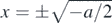 appear. If x stands for a field, e.g. the Higgs field, the appearance of the minima with a negative value of the potential means that the vacuum is not trivial but rather acquires a nonzero value of the field.
Examples of fold catastrophe systems have been reported in the literature. These include the motion of the Cartesian diver [8], whose explanation requires notions from mechanics and thermodynamics; a cylinder with a magnet inside placed in an incline and experiencing a constant magnetic field [9]—an example where mechanics and electromagnetism are involved in the explanation. Very recently, a pure mechanical example was presented [10], namely the study of tidal locking by analysing the effective gravitational potential of a two-body system with two spinning objects. It was shown that the effective potential may or may not develop a local minimum and a saddle point corresponding to a tidally locked circular orbits.
The system presented in this article is also purely mechanical, but much simpler. It is worth mentioning that the system is often evoked to establish a classical analogue in the explanation of the above mentioned Josephson junction effect (a pure quantum mechanical phenomenon) [11, 12]. The objective here is to present the experimental apparatus that we have constructed and to explore the interesting classical physics it can provide at an undergraduate level (or even pre-college). Interesting enough, a plenty of fundamental physics aspects can be addressed by studying a potential that plays a central role in the explanation of sophisticated aspects which are at the core of new technologies such as quantum computing.
The above mentioned fold catastrophe is very well exemplified and the amazing behaviour of the system is very well captured by the students in the classroom or by the audience, in general, playing a curious motivational role.
This paper is organized in the following way. In section 2 we describe the experimental apparatus and, in section 3, we describe its dynamics (translation and rotation). In section 4 we derive the effective potential for the system and next we explore several aspects of the catastrophic behaviour. In section 5 we summarize the main point of this experimental work.
2. Experimental apparatus
The system is shown in figure 1. Two equal ruler-shaped bars are tightly fixed on each side of a disk made out of a hard plastic, which may rotate without friction around its axis and acts as a pulley. A thread is wrapped around the pulley's rim and a body is hanging at its end. The system is mounted on a structure around 1 m high and tightly fixed on a table. The body may oscillate up and down under appropriate circumstances, or, under other conditions, it simply falls down, while the pulley and the bars perform complete turns around the axis (unstable mode). The pulley should lie at some 2 m high, for better visualization, but mainly because we want to allow the pulley to execute some three turns before the body touches the ground, when the system is moving in the unstable mode. It is recommended that some soft stuff be placed on the ground underneath the body in order to reduce the impact with it.

Figure 1. Mechanical apparatus for the study of the fold catastrophe: perspective view (left) and front and lateral views (right).
Download figure:
Standard image High-resolution imageFor the quantitative experiments, it is also useful to have several different bodies, each one with a fixed and known mass and one body whose mass can be easily modified by adding or removing, for instance, grains of lead.
In table 1 we give the data for our own particular device, but, of course, the actual design of this type of apparatus can be very variable. In the table we just present the magnitudes that are required, in the next sections, for the theoretical study of the system. The other elements are: the aluminum bars which are ∼3 cm wide and ∼2.5 mm thick, and the shaft which is a long screw attached to the disc, using a bearing taken from a spinner toy (it is amazing how friction in this bearing's toy is really so low). As shown in figure 1, the bars are mounted in such a way that there is room enough, when the parts of the system are moving, for the body to pass between them without being touched.
Table 1. Physical magnitudes, symbols and values, involved in the description of the experiment in the next sections.
| Name | Symbol | Value |
|---|---|---|
| Disc radius | R | 0.09 m |
| Disc mass | μ | 0.36 kg |
| Body mass | m | 0 ...0.40 kg |
| Length of the bar | L | 0.30 m |
| Mass of the (dual) bars | M | 0.23 kg |
This is a not very expensive experiment—the material used here was bought by less than 50 euros in a bricolage shop.
3. Dynamics of the system
As mentioned in the previous section, the experimental device consists of a disc of mass μ and radius R that freely rotates around its axis and acts as a pulley, a bar of length L and mass M attached to the disc (the fact that it is actually split into two equal bars is not relevant for the discussion), and a body of mass m hanging at the end of a long enough light thread to be wrapped around the pulley's rim several times. Figure 2 shows these three elements and the relevant forces for the study of the dynamics of each component. In the body, there is a force  exerted by the thread and the weight,
  . The forces responsible for the torque on the disc and the bar with respect to the disc axis, O, are the force
  exerted by the thread, and the weight of the bar,
  . To study the dynamics of the system one should consider, separately, the translational motion of the body, the rotational motion of the disc and the bar around O, and the corresponding oscillation of the disc and the bar. When the system is at rest, and there is no hanging body, the bar remains vertical. For the rotational and oscillatory motion, the angular position is described by the angle φ represented in figure 2. The body's position is described by x, the origin of the x axis being at the level of the free end of the thread when the body is not suspended, i.e. at φ = 0.
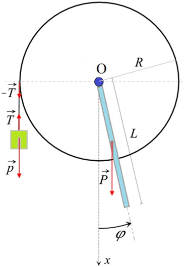
Figure 2. Sketch of the mechanical system with a disc, a bar attached to it and a hanging body.
Download figure:
Standard image High-resolution imageAssuming that the rope does not slide on the pulley's rim, the connection between the translation and the rotation is expressed by the geometrical relation

and, accordingly, v = Rω and a = Rα, where v and a are the velocity and acceleration of the body and ω and α are the corresponding angular magnitudes for the disc and the bar.
Applying Newton's second law to the body leads to

For the disc and the bar, one has

where

is the sum of the moment of inertia of the disc (first term) and of the bar (second term). For the latter, the Steiner's theorem [13] has been applied to obtain the moment of inertia with respect to O.
Friction and air resistance turn out to be negligible except for very long periods of the motion. In principle they can be added in equations (2) and (3).
We can now use (1) in the second term of equation (2) to obtain

which, in turn, can be inserted in (3), leading to

where we have introduced the total moment of inertia of the system (contributions from disc, bar and body, respectively)

and the constant

The angle φ0 corresponds to the equilibrium position (no angular acceleration) of the system. At this angular position the hanging body is at position x0 = Rφ0. Of course, equation (8) implies that an equilibrium position only exists for

Figure 3 shows three equilibrium positions for three values of A, out of which two are extreme values: A → ∞ (φ0 = 0°), A = 2 (φ0 = 30°) and A = 1 (φ0 = 90°). These positions correspond to three different masses of the hanging body. In the leftmost picture, the body is absent. In the rightmost picture the system is about to move (a tiny increment of the mass of the hanging body will make it to fall down). Apart of these stable equilibria, there exist, for each A, unstable equilibria at φmax = π − φ0.
Figure 3. System in static equilibrium at three different positions.
Download figure:
Standard image High-resolution imageIn the next section we derive the potential energy for the system, recognizing that A is a control parameter, and analyse both the statics and the dynamics of the system.
4. Fold catastrophe potential
As for many other systems, the energy approach allows us to discuss interesting aspects of the problem. We assume that the friction and resistance forces are negligible and we can write the gravitational potential energy associated with the body + bar (the centre of mass of the disc does not move) as a function of φ:

where the origin of the potential energy, U(0) = 0, has been fixed at φ = 0 (equivalently, x = 0).
For the physical discussion, it is more appropriate to introduce an 'adimensional potential' defined by

which can then be written as

where A is the adimensional parameter (9).
The introduction of adimensional quantities is not mandatory but facilitates the analysis. The potential (12), known as washboard potential, is of the same type of the one found in [9], then for a system very different from the present one: there, the motion in an incline of a cylinder with a magnet inside, subjected to a magnetic field, was considered.
In figure 4 we plot the function (12) and it is clear why A is a control parameter. For A > 1, there are local maxima and minima, which merge together as A decreases towards 1. The function extrema are obtained from the condition

which leads to

consistent with the previous definition of A, equation (9). For A = 1, the maxima and minima become stationary points. For A < 1, the static equilibrium referred to at the end of the previous section is no longer possible, the body falls all the way down while the disc and the bar execute successive full rotations. The transition from the static equilibrium possibility to the situation where that is impossible is a characteristic of the fold catastrophe potential. The transition is controlled by A, hence its name 'control parameter'. We can establish the relation between the potential (12) and the fold catastrophe potential, U(x) = x3 + ax, mentioned in the Introduction, by expanding V(φ) in Taylor series around  , with
  . We find
or, up to third order,

with  . We conclude that the control parameter a corresponds to


Figure 4. Adimensional whasboard potential, V, as a function of φ.
Download figure:
Standard image High-resolution imageThe catastrophic behaviour of the potential can also be recognized by studying the dynamics of the system, which is also very interesting, namely for A > 1. In figure 5 we show the function V(φ), for A = 4, with the insertion showing the potential near the minimum, φ0 ∼ 14.5°, exhibiting a clear parabolic form.
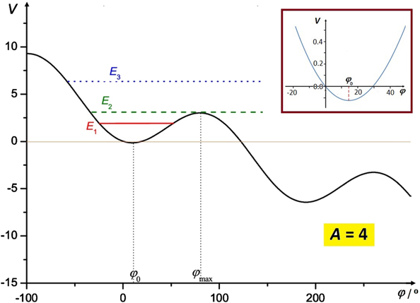
Figure 5. The adimensional potential for A = 4, with the insertion showing it near a minimum.
Download figure:
Standard image High-resolution imageAround the minimum, the oscillations are harmonic and their frequencies can be obtained from equation (6). To study the small oscillations around φ0 it is convenient to introduce the small angle ϕ = φ − φ0 ∼ 0. The expression in parenthesis on the right-hand side of equation (6) may then be written as

and that equation, for the small oscillations around φ0, becomes a harmonic oscillator like equation:

The angular frequency squared is explicitly given by

When the body is absent, the equilibrium angle is φ0 = 0 and this frequency reduces to the one for the physical pendulum. For any angle φ0, the period can be experimentally obtained directly with a chronometer and compared with the theoretical value  . With our device, we obtained for the period the results presented in figure 6, with a better correspondence for smaller angles. Since the mass in the disc is not uniformly distributed, with a metallic central part (the bearing and the piece where it fits inside), we have used the experimental moment of inertia I' of the disc + bar, measured for φ0 = 0, and not directly using equation (4). With I' taken to fit the first experimental point, the theoretical prediction for the function T = T(φ0) is the curve shown in figure 6.
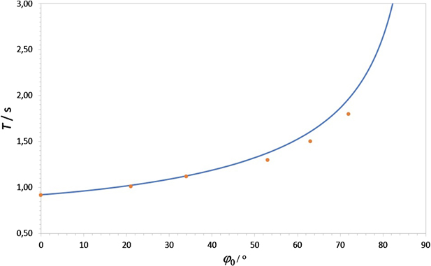
Figure 6. The period for small oscillations as a function of the equilibrium angle. The blue curve is the theoretical prediction.
Download figure:
Standard image High-resolution imageIf the energy is well above the local minimal energy, as E1 in figure 5, the system performs stable non-harmonic oscillations. The initial energy of the system can be easily varied by moving it away from the equilibrium position and/or by giving it an impulse, either on the hanging body or on the bar. For oscillations around φ0, there is a critical energy, E2, for the system to move in the stable mode. If the energy is increased even infinitesimally beyond this value, the oscillatory regime ceases and the body falls down. For even higher energies, such as E3, the only possible motion is of this very same type (unstable mode). In the classroom or in a demonstration in general, it is amazing to observe the change from one type to the other type, just by changing the initial condition. This is again a characteristic of the fold catastrophe potentials.
It is interesting to notice that studying small deviations around the maximum leads to the same equations as for the minimum, with the only exception that cos φ0 becomes negative. As a consequence, the right-hand side of equation (19) changes sign, while the final expression for ω2 in (20) remains the same. The solution can be cast in the form ϕ(t) = aeωt + be−ωt . Depending on the initial conditions, the system may either start to oscillate around the minimum with a large amplitude, or to accelerate, with both, the displacement and the velocity, increasing exponentially.
Another activity related to the device, that can be carried on by students, is the numerical integration of the equations of motion, using a simple method, such as the Euler algorithm. This can easily be done, for instance in Excel® or equivalent, a platform with the advantage of a very good graphical interface. Just by slightly changing the control parameter in the vicinity of the critical value, the student may amuse himself with the different possible solutions—oscillatory or no-return. The same applies for A > 1, now by changing a kinematic parameter, such as the initial position or velocity, upon which the total mechanical energy depend. The passage from stable oscillations to the unstable regime can be visualized in successive 'numerical experiments'. The v(t) or x(t) graphs for both the oscillation and the no-return modes are similar to the ones presented in [9] for the cylinder in an incline, though the damping now is much lower. These functions can be directly compared with the real ones obtained using a camera and an appropriate software such as the Tracker (which is free) [14]. In particular, one can follow the evolution of the system starting from the maximum, e.g. releasing the bar at the unstable equilibrium position. In this case, for sufficiently short times, the displacement of the body behaves as x(t) ∝eωt and the velocity as v(t) = ωx(t) as shown in figure 7.

Figure 7. The displacement (full circles), the velocity (open circles), their ratio, multiplied by 10 (squares), of the body starting from the maximum, and the theoretical value of this ratio, ω.
Download figure:
Standard image High-resolution image
A final suggestion refers to simulations. We believe that the present study provides a good opportunity for setting up a simulation. With this respect, it is worth mentioning that the kinematics of our system is similar to the one described in [9], for which a very interesting and pedagogically valuable simulation has been done by Ángel Franco García [15].
5. Conclusions
At the end of previous section we offer a non-comprehensive list of suggestions to explore the device. In this paper, we do not provide a lab protocol for a concrete experiment. Rather, our intention is just to present the device, to give concrete ideas for its construction, while stressing the wonderful underlying physics. The related potential is relevant because, on the one hand, it constitutes a clear example of a potential showing a fold catastrophe behaviour; and, on the other hand, it turns out to be the potential that is used to describe the Josephson junctions behaviour, with the already mentioned implications for the qubits circuits in quantum computing. The apparatus studied in this work is well known exactly because it is many times mentioned to establish a classical analogue to the elements of the Josephson junction circuit.
Acknowledgements
MF and RN are grateful to the Portuguese Physical Society and to the Royal Spanish Physical Society for the invitations to deliver talks during their national meetings on 'Catastrophic potentials'. These talks were motivational to write the paper.