

Abstract
The aim of this study is to investigate the bouncing dynamics of a small elastic ball on a staircase consisting of rounded edge steps, as an example of a dissipative gravitational billiard, and to determine if its dynamics is chaotic. We derive a nonlinear recursion for the coordinates of the collisions, completed with numerical simulations, which indicate that the bouncing dynamics is chaotic, as also follows from elementary considerations regarding the Lyapunov exponent. It is, however, surprising that instead of permanent chaos, only the transient form is present. The main reason behind this is that a collision with the rounded edge of the step enhances the horizontal velocity leading to larger and larger jumps. Not even the introduction of a tangential coefficient of restitution (COR) on the curvature can hinder the flying away of some trajectories. There is also a chance for remaining trapped on a single step in the form of sliding, representing another possibility for escape. Therefore, chaoticity holds for long trajectories before any kind of escape takes place. We also show that an impact-velocity-dependent COR converts the dynamics to permanently chaotic with an underlying fractal attractor. Only elementary mathematics is required for the analytic calculations used, and we offer a set of problems to solve, as well as a user-friendly demo software on our website: https://theorphys.elte.hu/fiztan/stairs to facilitate experimentation and further understanding of this complex phenomenon.
Export citation and abstract BibTeX RIS

Original content from this work may be used under the terms of the Creative Commons Attribution 4.0 licence. Any further distribution of this work must maintain attribution to the author(s) and the title of the work, journal citation and DOI.
1. Introduction
In an Austrian high school textbook the bouncing motion of a ball down a staircase is given as one of the real life examples of chaotic dynamics [1]. This statement was investigated from a theoretical/numerical point of view in a previous paper [2] in the case of rectangular steps consisting of horizontal and vertical parts only. The authors, in order to keep the model as simple as possible, assumed the ball to be a non-rotating point, the air drag negligible, as in billiards (see e.g., [3]), and the bounces to occur elastically with some energy loss, described by a constant coefficient of restitution (COR), k < 1. The motion was found to be nonchaotic (typically quasi-periodic), therefore, here we turn to the question of whether by keeping the framework of gravitational billiards, that is point-like non-rotating ball with negligible air drag in a gravitational field (see e.g. [4–6]), a mere change in the geometry, namely the rounding of the edges (resulting in what we call rounded stairs in short), is sufficient to generate chaos. Intuitively, this is a natural expectation, and the authors of [2] conjectured indeed that the dynamics will be chaotic since the curvature at the edge will act as a magnifying mirror, which scatters parallel incoming beams (while the rectangular case contained only plane mirror-like surfaces).
We provide an elementary argument indicating that a standard chaos quantifier, the so-called Lyapunov exponent of long-lasting motions is positive, no matter how short the curvature at the edge is. There is thus potential for chaos from even the smallest possible amount of rounding. The numerical simulations provide, however, a tricky detail: instead of permanent chaos, only the transient form of chaos shows. The main reason behind this is that a collision with the curvature enhances the horizontal velocity of the ball, hence the jumps become larger and larger. Not even the introduction of a new source of dissipation, a constant tangential COR, can make the dynamics to be bounded. Besides this escape to infinity, there is also a chance for remaining trapped on a single step in the form of sliding. There are thus two sources of escape, and we show that long-lasting motions are indeed chaotic before any type of escape takes place.
An elementary definition of chaos states that it is a long-lasting motion which is irregular in time; sensitive to initial condition; complex, but ordered, and associated with a fractal structure in the phase space (for more details see the textbook [7]). We provide evidence for each of these fundamental properties of chaos.
The investigation of the physics behind the concept of CORs [8–12], and its dependence on different parameters is a current problem of interest. There are indications for the CORs being dependent on the impact velocity since internal degrees of freedom might become excited upon highly energetic impacts [13, 14]. After considering the CORs constant in both the normal and the tangential directions, we also turn to a version when the tangential COR on the curvature is velocity-dependent. By phenomenologically choosing a simple exponential decay, we find that both kinds of escape can be avoided, and the bouncing dynamics becomes permanently chaotic with a fractal attractor in the phase space.
The theory of transient chaos is well established (see e.g., the monograph [15]), and is not without any technically demanding methods. In order to make the approach feasible for undergraduates, we are applying here only the simplest available techniques, and keep the material on the level of the introductory textbook [7]. We offer the exploration of the dynamics on the rounded stairs with different COR values as a useful project for undergraduates, supported by a set of problems to solve, and a demo software freely available on the internet for personal experiences with different facets of the motion 4 .
2. A short summary of the dynamics on rectangular stairs
In [2], a rectangular staircase was considered with step tread L and rise M, tilted from left to right. The main findings turn out to be reproducible by considering the bouncing of a ball on a slope but letting energy loss occur only in the vertical velocity component.
A ball initiated with a horizontal and vertical velocity u0 and v0, respectively, collides with a surface of slope m after time

with vertical velocity

Problem 1. Based on the rules of oblique projection, derive these relations.
These relations apply with good accuracy to a staircase of slope m = M/L. Since, however, the collision occurs there with a horizontal plane, only the vertical velocity changes upon collision. In the presence of a COR k < 1 for this component, the rebound velocity right after the bounce is

After some time, a stationary sequence of bounces sets in whose average velocity  can be obtained from the condition of repetition:
  (both for the slope, on which strict repetition occurs, and for the staircase), leading to

The appearance of factor u0 suggests that velocities are worth measuring in units of the initial horizontal velocity (which remains constant for the rectangular staircase as no force acts on the ball in this direction).
The average flight time between two bounces follows from (1) applied with  instead of v0. Substituting this time into the function u0
t of horizontal displacement, we obtain the average number
instead of v0. Substituting this time into the function u0
t of horizontal displacement, we obtain the average number  of stairs between two bounces as

This expression contains an important dynamical parameter

a dimensionless expression of the gravitational acceleration in combination with the horizontal initial velocity and the step tread L.
According to [2], these formulas provide good approximations for any k, down to k = 0.4 where their validity is lost because with such strong dissipation all balls might become trapped on a single step, stop bouncing, and start a sliding motion. The majority of the long lasting bouncing motions is quasi-periodic (i.e., they repeat themselves with some mismatch), and expressions (4) and (5) yield the average velocity and jump number over the quasi-periodic motion. Strictly periodic bouncings occur at exceptional, discrete values of k, where expressions (4) and (5) might become exact.
With parameters m = 1/2 (a typical slope of staircases), H = 4 and a COR value k = 0.6 a periodic bouncing occurs with a single bounce on each step ( ), while the case k = 0.75 corresponds to a typical quasi-periodic motion (
 ). For the dynamics on the rounded stair we shall keep m = 1/2, H = 4 fixed, and use these COR values throughout. The user of the simulation on our webpage can, however, freely set these parameters, and the others, too.
Problem 2. How long is the tread if H = 4 and the initial horizontal velocity is 1 m s−1? For which initial velocity would H be as small as 0.0625 on this staircase?
3. Bouncing on the rounded stairs
3.1. The shape of the staircase
Each step consists of a horizontal and a vertical part, connected smoothly with an arc formed by a quarter of a circle of radius R. Relations (5) and (6) of the previous section imply that it is worth measuring all lengths in the unit of the step tread L. In this representation the steps are of unit length, and of rise m = M/L, while the radius of the arc is r = R/L, so that the horizontal part of a step is of length 1 − r, as figure 1 indicates. We shall be interested in the range 0 < r ⩽ 0.2. The figure also contains the schematic trajectory of a ball, and the quantities needed for a unique description of the bouncing dynamics are also given.
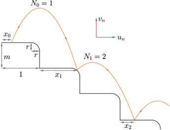
Figure 1. Shape of the rounded staircase, and the trajectory of a ball bouncing down it. Quantities characterising the motion are: the location of the nth collision, xn , the vertical and horizontal velocity after the bounce vn and un , respectively, measured in units of the initial horizontal velocity, while the number of steps the ball jumps over between the nth and n + 1st collision is Nn .
Download figure:
Standard image High-resolution image3.2. Monitoring the motion on this staircase
Our goal is to find a relation between the location and velocity data of the nth and the n + 1st bounces. Velocities are convenient to measure in units of the initial horizontal velocity u0, as e.g., (4) suggests. From now on, the rebound velocities un and vn , right after the nth bounce, are considered to be dimensionless. The only quantity in which the dimensional u0 appears is the dynamical parameter H given by (6). From the dimensionless data xn , un , vn of the nth bounce, we would like to know those of the next bounce, i.e. we determine the mapping

The y coordinates do not appear here since on the staircase this is never an independent quantity, it follows from the x coordinate and the shape of the stairs. Initial data of the entire motion are represented by n = 0. An important auxiliary quantity is the jump number, Nn , expressing how many steps are jumped over between the nth and the n + 1st collision. Relation (7) concentrates only on the bounces but, if desirable, the continuous-time motion can be reconstructed from these data in the form of parabola arcs.
To keep things simple, we place the origin of our coordinate system to the left edge of the step on which the collision occurs. This means that we always shift the coordinate x of the collision back to the unit interval, and the y coordinate is either zero (if the bounce is on the horizontal part of the step), or negative. As in the rectangular case, air drag is assumed to be negligible.
To simplify the monitoring process, we cut the trajectory into two pieces: the first one lasts until the ball hits an imagined rectangular step at some coordinate  (see figure 2), because the impact data here can be determined analytically, and the rest, until the real bounce with the step at some xn+1 occurs, to which numerical methods should be applied
5
.
(see figure 2), because the impact data here can be determined analytically, and the rest, until the real bounce with the step at some xn+1 occurs, to which numerical methods should be applied
5
.
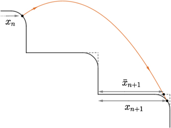
Figure 2. The trajectory of the ball between two collisions. The x coordinate of an imagined bounce with the rectangular stairs,  , can be calculated analytically, but this need not be the x coordinate, xn+1, of the actual collision.
Download figure:
Standard image High-resolution image3.3. Analytic part
Let the motion, right after the nth bounce, start on a step at dimensionless horizontal coordinate 0 < xn
< 1. The corresponding y coordinate is  if the bounce has been on the curvature of the step (xn
> 1 − r), and yn
= 0 otherwise. After the start with horizontal and vertical velocity components un
and vn
, respectively, we consider the stairs to be rectangular, and assume that the number of steps,
if the bounce has been on the curvature of the step (xn
> 1 − r), and yn
= 0 otherwise. After the start with horizontal and vertical velocity components un
and vn
, respectively, we consider the stairs to be rectangular, and assume that the number of steps,  , flown over until the next collision with this imagined staircase is known. Thus the collision will happen at a depth
  , and all the quantities characterising this collision can easily be determined from the laws of oblique projection. The results are marked by a tilde to indicate that these are not necessarily the data for the collision with the rounded stairs. For the x coordinate one obtains

where

and the square brackets represent the integer part. The jump number  is the smallest integer for which equations (8) and (9) possess a solution. The impact velocities (marked with commas) with this
  can be expressed as

For yn = 0 these relations provide the exact description of the bouncing on rectangular stairs, as given in [2] where tildes are not used as the results always describe the state at the moment of a real collision.
3.4. Numerical part
In the case of  , numeric calculations are required. We consider the moment when the ball reaches the imagined rectangular stair, to be at time t = 0 for the subsequent treatment. This way, the x and y coordinates of the ball can be determined as functions of time: x(t), y(t). The y coordinate of the stair is a function of x, but when calculated at the time dependent x(t) coordinate of the ball, it will practically become a function of time, telling us the height of the stair at the point directly underneath the ball at any given moment. Subtracting this from the ball's height, y(t), we get the vertical distance Δy(t) between the ball and the stair.
Problem 4. Determine the function Δy(t).
The numeric algorithm checks this quantity after every small time increment Δt, at t = 0, Δt, 2Δt, ... to see its sign. When Δy(t) becomes negative, it indicates that the collision has happened prior to that moment. Hence, we return to the last instance t of time that gave a positive value and start using a smaller increment Δt' that we conveniently choose to be one tenth of Δt. The process continues, now checking after every increment Δt' until we run into another negative value for the vertical distance of the ball and curvature. An even smaller increment can be chosen, and the same steps can be executed several times, to achieve a sufficiently accurate determination of the time t* that passes between the ball being on the imagined rectangular stair and colliding with the actual one. We have the error, the shortest increment used, be below 10−14. 6 We have experienced with other increments, too. By choosing this error to be ten times smaller, i.e. 10−15, the deviation in the values of xn , un , vn was found to be typically of order 10−11 or less, even at collision numbers n above 100. We, therefore, decided to stick to 10−14. Another way to show the consistency, was to check that the results of [2] are recovered for r = 0. It is worth mentioning here that chaotic systems are error-magnifiers [7], thus errors unavoidably grow in the long-term dynamics, and the well-known chaos quantifier, Lyapunov exponent, is just the rate of this growth (see more about this in sections 4.4, 4.5 and 6). For this reason all long-term quantities should be given as averages, that do not depend on individual details. The Lyapunov exponent, too, is itself a kind of average.
This done, the ball's position,  , and impact velocities as
  ,
,  are also known.
In the simplest scenario, the ball bounces on the same step as it would if the stairs was rectangular, just lands on the curvature instead of the horizontal surface (see figure 2). Occasionally, the ball can 'skip' a step, when the value of  derived via the analytic calculations is not the actual value of Nn
. In this case, the ball misses the curvature of the step that it would have hit if it were rectangular. Since the trajectory of the ball does not intersect with the curvature, the numeric algorithm will not find a solution. This problem can be eliminated by constantly checking the inequality x(t) < 1, and whenever it becomes incorrect, it is certain that the ball has 'skipped' the step. Then, we return to the analytic calculations, substituting
derived via the analytic calculations is not the actual value of Nn
. In this case, the ball misses the curvature of the step that it would have hit if it were rectangular. Since the trajectory of the ball does not intersect with the curvature, the numeric algorithm will not find a solution. This problem can be eliminated by constantly checking the inequality x(t) < 1, and whenever it becomes incorrect, it is certain that the ball has 'skipped' the step. Then, we return to the analytic calculations, substituting  as the new value of
  . Although plausible, seldom does the ball 'skip' two or more stairs this way, nevertheless, the same process of switching between analytic and numeric calculations can then be performed multiple times.
The output of the numerical part is the position xn+1 of the n + 1st collision, and the components u'n , v'n of the impact velocity.
3.5. Bounces
The collision rule can be described analytically. If the collision occurs on the horizontal surface, the vertical impact velocity v'n < 0 becomes multiplied by COR k < 1, and changes sign. The horizontal velocity remains unchanged, the collision rule is thus

On the curvature, the collision rule is naturally formulated in normal/radial and tangential components denoted by vr and vt, respectively. Here, k is applied for the normal component, thus we call it the normal COR. As will be seen later, it is worth considering the effect of another COR, the tangential COR, whose value will be denoted by j ⩽ 1. In terms of physics, this is a consequence of the collision not being instantaneous, thus forces are present while being in contact. The relevance of such a COR has been shown experimentally [18, 19]. We are here offering an elementary argument for its existence, which is based on the presence of a friction force during the short duration of contact. Let Ff,n (t) denote the magnitude of this force at the nth collision which always points against the tangential component of the velocity (see inset to figure 3), and is thus negative. Its time-dependence is not known, but thanks to Newton's second law this is not even needed to determine the momentum loss. The latter is given by
where the integral is taken over the time of contact, pt is the tangential momentum, and the momentum difference Δpt,n is negative. We consider the impact velocity v't,n to be the one right before the contact, and vt,n+1 the one at the end of it. The letter is the rebound velocity with which the flight of the ball starts. For a point of mass m* (not to be confused with m, the slope of the staircase), the tangential momentum difference is

The tangential COR j < 1 is thus set by the time integral of the friction force (and the mass), but, for simplicity, we will consider it a constant. For completeness, we mention that in models taking into account the internal structure of the ball, the tangential COR also depends on the internal details [20, 21]. 7 The tangential COR is applied only on the curvature in order to recover the dynamics of [2] with no curvature, r = 0.
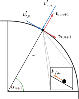
Figure 3. Schematic diagram illustrating the collision rule for a bounce occurring in a point of impact angle αn+1. The inset indicates the friction force acting during the impact.
Download figure:
Standard image High-resolution imageAll in all, the collision rule on the curvature is that for impact velocity components v'r,n < 0, v't,n , the same components right after the collision become (see figure 3)

The numerical part provides, however, the impact velocity in rectangular components as u'n = un , v'n with the coordinate xn+1 also given. If the bounce is on the curvature, xn+1 > 1 − r, the angle αn+1 under which the collision point is seen from the centre of the circle defining the rounding is obtained from (see figure 3)

The αn+1 is called the impact angle.
We thus have to transform the impact velocity into polar components in a frame of polar angle αn+1. Then (12) is applied with these components, and the new velocity components are transformed back in rectangular coordinates. For these rebound values un+1, vn+1 we obtain


Problem 5. Derive relations (14) and (15).
Problem 6. Determine the smallest impact angle αc permitted in (14) and (15) for given impact velocity components un ' and vn '.
Relation (14) clearly shows that, in sharp contrast to perpendicular stairs, the horizontal velocity component does not remain constant on the rounded stairs.
By the end of these calculations, we obtain the location of the n + 1st bounce, and the velocity components right after the collision, i.e. map (7) is completed. From here on the algorithm can be iteratively repeated an arbitrary number of times.
4. Bouncing on stairs with very short rounding
4.1. First observations
In this special case, collisions with the curvature are rather rare, the motion is mostly dominated by long sequences of the ball bouncing only on the horizontal part of the stairs. The numerical simulation on such a stair of rounding radius r = 0.01 also illustrates (figure 4) that without an energy loss in the tangential velocity, j = 1, the horizontal velocity, u always increases. This tricky feature indicates a strong deviation from the rectangular case.
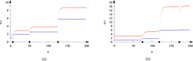
Figure 4. Time series of the two velocity components un (blue) and vn (red) up to 200 bounces on a stair of r = 0.01 with COR k = 0.6 (a) and k = 0.75 (b) and j = 1 in both cases. The initial coordinate is x0 = 0.53 in (a), and x0 = 0.76 in (b), while (the dimensionless) v0 = 3, and the parameters are m = 1/2, H = 4 here and throughout the paper. Instances of bounces with the curvature are denoted by dots along the n axis.
Download figure:
Standard image High-resolution imageAfter a bounce on the curvature, there is a jump in the u-component, while in vn a transient increase can be observed over about 10 bounces, after which a plateau follows.
Problem 7. At collisions with the curvature, why do we see red dots below the level of the previous plateau?
From here on the motion is like on the rectangular stairs. Since long sequences exist without the ball visiting the curvature, we can interpret the findings by considering un+1 right after the first hitting of the curvature as a new initial velocity u'0. In view of the definition (6) of parameter H, there is a new, smaller value  governing the motion leading, in view of (4), to average vertical velocity
  . The plateau after the first bounce corresponds to the attractor
8
, described in [2], belonging to parameter H' on the rectangular stair. The fine structure in the red lines of figure 4 indicates that the motion is quasi-periodic, although the stationary motion on the rectangular stair with H = 4, k = 0.6 (panel (a)) is periodic. The first plateau is, however, of finite length, after some time a bounce occurs on the curvature again, leading to a new initial velocity u''0 > u'0 for the forthcoming motion with an even smaller H''. The sequence of u0, u'0, u''0, ..., is increasing, indicating that the velocities are ever increasing, and larger and larger jumps occur. There is a tendency for an inherent instability in the system.
. The plateau after the first bounce corresponds to the attractor
8
, described in [2], belonging to parameter H' on the rectangular stair. The fine structure in the red lines of figure 4 indicates that the motion is quasi-periodic, although the stationary motion on the rectangular stair with H = 4, k = 0.6 (panel (a)) is periodic. The first plateau is, however, of finite length, after some time a bounce occurs on the curvature again, leading to a new initial velocity u''0 > u'0 for the forthcoming motion with an even smaller H''. The sequence of u0, u'0, u''0, ..., is increasing, indicating that the velocities are ever increasing, and larger and larger jumps occur. There is a tendency for an inherent instability in the system.
As the parameter H changes, the spectrum of the discrete k values that result in periodic motion changes with it, thus making it statistically impossible for periodicity to occur after a bounce on a curvature. This also implies, that motions for k = 0.6 are no longer fundamentally different from those for k = 0.75. So much so, that it should not be treated as a separate case, as all of our results for k = 0.75 similarly hold for k = 0.6. It is more practical to analyse motions that start with parameters inducing quasi-periodicity because then the ball will eventually bounce on the curvature under every initial condition (in contrast to motions with parameters of periodic motions, when only a portion of the initial conditions do so, as it can only happen before the periodicity sets in). For this reason we decide to keep only the COR value k = 0.75 in what follows.
4.2. Analytic investigation of the horizontal velocity change
The well-known property of an absolutely elastic ball bouncing down on stairs, namely that its jumps are ever increasing (since the potential energy is decreasing on average, but the total energy is constant), appears to remain valid on rounded stairs even in the presence of a normal COR. This COR is unable to lead to a sufficiently strong energy loss to oblige the kinetic energy to stay on average. The tendency of increase follows from relation (14) without tangential energy dissipation (j = 1).
Problem 8. Show, based on relation (14), that with j = 1, the horizontal velocity can never decrease: un+1 ⩾ u'n = un .
The inclusion of a tangential COR j < 1 provides a stronger dissipation, and there is a chance for having smaller horizontal rebound velocities then impact ones. A consequence of (14) with j < 1 is that un+1/u'n ⩾ j.
Problem 9. Show, based on relation (14), that its maximum is taken for an angle α* = π/4 + αc /2, i.e. for the average of the permitted angles in (αc , π/2). The minimum is achieved at the two ends αc and π/2, where un+1 = jun .
When analysing the velocity ratio un+1/u'n
a difficulty is that it contains v'n
/u'n
, a quantity not known analytically. In the limit of small r, however, there is a possibility for simplification: there are long stretches of bounces occurring only on the horizontal parts of the steps, and therefore, between two collisions with the curvature the results of section 2 apply. It is sure that after an impact with v'n
, the rebound velocity is −k
v'n
which, after the transients, takes one of the values for a typically quasi-periodic bouncing. Their average is given by (4). Therefore, −k
v'n
can be approximated by  in which u0 should be taken as the horizontal velocity after the last collision with the curved surface, i.e. u'n
in the current notation. We can thus write
in which u0 should be taken as the horizontal velocity after the last collision with the curved surface, i.e. u'n
in the current notation. We can thus write

Substituting this relation into (14) we obtain

The advantage of this approximate relation is that the velocity ratio appears as a one-variable function of the impact angle αn+1.
Problem 10. Based on (16), determine the critical angle αc as a function of the parameters m and k. What is this angle for m = 1/2 with our baseline COR value k = 0.75?
In figure 5 we plot the velocity ratio (17) as a function of the impact angle, for different values of the tangential COR j. We see that the velocity ratio can be both smaller and larger than unity, and for sufficiently low values of j the average can be close to unity. For k = 0.75 such a value is j = 0.2. A balance between increased and decreased rebound u values can only be ensured with rather strong tangential momentum loss. We shall use the mentioned j in what follows.
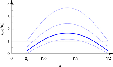
Figure 5. The velocity ratio un+1/u'n as a function of the impact angle according to relation (17) with k = 0.75 and (from top to bottom) j = 1, 0.5, 0.2, 0. The curve belonging to a balanced case, with a mean value close to unity (j = 0.2) is marked with a bold line. The smallest permitted angle, αc is indicated.
Download figure:
Standard image High-resolution image4.3. Lifetimes
Even if a tangential COR is applied at which the average velocity ratio un+1/un ' is close to unity (like e.g. the j value represented with the bold line in figure 5), there always exist initial conditions which lead, sooner or later, to an ever increasing sequence of u. For large velocities, however, the air drag cannot be neglected, although our reasoning is based on the rules of oblique projection. We are thus running out of the validity of our model if the velocity is too large. To avoid this, we stop considering the results reliable if the collision data exceed a threshold value. For practical reasons, we prescribe a threshold in the jump number, Nth = 100.
Whenever Nn is larger than this, simulation is stopped and we say that the ball has flown away. As an arbitrary long monitoring of the motion is not possible within the model, chaos, if present, can only appear as a transient. The theory of transient chaos [7, 15] requires the existence of long lasting motion, we shall, therefore, be after trajectories remaining well defined over several hundreds in n at least.
Problem 11. The threshold in the jump number implies a threshold in the velocities, too. Based on (5) and Nth = 100, show that for k = 0.75 uth ≈ 7.5.
For other initial conditions, the ball, after a period of bounces on different steps, might undergo an infinite number of collisions on a single step. Parallel to this, the sequence of vn tends to zero. This indicates the turning of the bouncing motion into a different kind of motion: sliding. Such cases provide another kind of escaping process, and we say the ball has stuck down. Numerically, simulation is stopped when either of the velocity components become less then 0.01 after a bounce on a horizontal part of a step. Sticking is a well-known phenomenon for bouncing balls (see e.g. [23–26]) but was found in [2] to exists only for k < 0.4. It is the presence of another source of dissipation, described by j, which leads to sliding even for larger k values in our cases.
Problem 12. The lowest graph of figure 5 represents parameter sets where practically no increase would occur in the horizontal velocity. Why do not we choose such COR values to prohibit balls flying away?
We are thus interested in long lasting sequences of bounces before flying away or turning to sliding. For small r there is a wide range of such initial conditions. An interesting pattern arises if we examine the total number of bounces τ before any kind of escape takes place, and plot this lifetime as a function of the initial position along the step. Red and blue columns mark motions which end in flying away and in sliding, respectively. Figure 6 exhibits an intricate pattern: the heights, the lifetimes before escape, are irregularly distributed, and the change of colouring is also irregular.

Figure 6. Lifetime τ vs initial position x0 for r = 0.01 and k = 0.75, j = 0.2. (a) The distribution of lifetimes on the unit interval, in 100 starting positions. (b) The same on a tiny interval of length 2 × 10⁻⁴ around x = 0.36 in 100 points. Columns higher than 8000 are cut at 8000.
Download figure:
Standard image High-resolution imageTo gain more insight, we select a tiny, hardly visible interval around x = 0.36, zoom in on it, and plot the lifetimes on it in panel (b). The structure is very similar to that of in panel (a), no regularity occurs on fine scales. Statistical features, like e.g. the ratio of flying away and sliding remain the same (roughly 1 to 2).
The irregularity of the distribution both in height and colour provides an example of sensitivity to initial conditions, a general feature of chaos, while the fractal-like pattern in the lifetime distribution is a property characterising transient chaos specifically [7, 15].
4.4. Elementary estimation of the Lyapunov exponent
The presence of a curved surface act as a convex mirror and scatter the beam of balls falling on it along parallel paths. This tendency for divergence serves as the source of chaos in the motion of the balls. A measure of the strength of this sensitivity to initial conditions is the so-called Lyapunov exponent (see [7, 22]). This also quantifies the growth of small initial errors as time progresses. An elementary argument for its estimation is as follows.
Consider two balls hitting the curvature of radius r along parallel paths and with approximately the same velocity. The impact points are close to each other and the corresponding impact angles αn+1 differ by some small Δα. The rebound directions will be different, characterised by a relative angle Δφ (see figure 7). It is intuitively clear that these two small angles are proportional to each other:

where a is a proportionality constant.

Figure 7. Schematic diagram illustrating the concepts of the angle differences Δα and Δφ for bounces on a circular arc of radius r.
Download figure:
Standard image High-resolution imageProblem 13. Determine coefficient a in (18) for collisions with CORs k and j.
Because of the divergence in their path, the distance Δx between the balls increases in time. As an estimation, we can write this distance as Δx = Δφ ⋅ s after a length s along the paths. We take s to be of order unity, i.e., corresponding to the length of a single step. Rearranging this as Δx = Δφ ⋅ r/r = Δα ⋅ r ⋅ a/r, and using that Δα ⋅ r = Δx0 is approximately the initial distance between the balls, we find Δx = Δx0 a/r. This distance increases by a factor of a/r. The logarithm of this, ln(a/r) can be considered the Lyapunov exponent belonging to a bounce on the curvature. Hitting this part is, however, rather rare (at least for small r), and the corresponding probability is expected to be proportional to r (as the step tread is chosen to be unity). We thus can write the average Lyapunov exponent as

where c > 0 is a proportionality constant. For r << 1, the logarithm ln(a/r) = ln a − ln r is dominated by ln r and the expression simplifies to

This result indicates that the knowledge of constant a is not necessary in this limit. For r → 0 the Lyapunov exponent vanishes in harmony with finding no chaos on the rectangular stairs in [2]. The illuminating feature of (20) is that it provides a positive value for any r > 0. There is thus a potential for chaos on any rounded stairs, no matter how small r is [27].
4.5. Numerical determination of the Lyapunov exponent
We divide the unit interval in 106 pieces and initiate from all these x0 coordinates a trajectory (with (dimensionless) velocity v0 = 3). The distance Δxn
between originally neighbouring pairs of initial distance Δx0 = 10−6 is numerically followed as a function of the number of bounces, n. In order to keep only pairs with long lasting motion, we keep only those which possess at least 1000 bounces. The logarithm ln Δxn
of the distance is taken from each of the 76 674 pairs kept. The average of these,  , is evaluated and plotted as a function of n in figure 8. The growth of this quantity (indicating an approximately exponential increase) is a clean sign of sensitivity to initial condition, i.e. of chaos. The slope (after discarding the initial transient of 30) is the Lyapunov exponent. Its value is obtained as λ = 0.176 ± 0.004. Although (20) need not hold since r = 0.01 is small but not very small, a comparison is worth while: r ln(1/r) = 0.046 for r = 0.01, not the same as the numerical value but certainly on the same order of magnitude. (If (20) is taken seriously, the proportionality constant is c ≈ 4.)
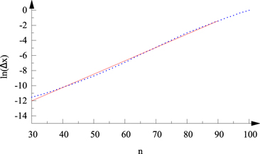
Figure 8. The average of logarithmic distances ln Δxn of 76 674 pairs of initial distance Δx0 = 10−6 vs n(k = 0.75, j = 0.2, r = 0.01). Only pairs with at least 1000 bounces have been kept when performing the average. The straight line fit is marked by a red line. The deviation from linearity for n > 90 is due to the fact that the pairs are strongly deviated, their distance is on the order of the step length, unity, and, accordingly, their logarithm is close to zero.
Download figure:
Standard image High-resolution image4.6. Patterns in phase space and real space
Chaotic motions are accompanied with intricate patterns in the phase space. In our model the phase space is three-dimensional with variables as appearing in mapping (7). We shall investigate two projections, the (un , xn ), (vn , xn ) phase planes. We saw that there is a convergence time on the order of 10 bounces to reach a kind of stationary motion, therefore we cut the first 30 iterations of long trajectories. The last 30 iterations are also cut in order to avoid points characterising the escape process. One example of such trajectories is shown in figure 9.

Figure 9. Phase space patterns in the (v, x) (a) and (u, x) (b) planes for r = 0.01 and k = 0.75, j = 0.2 arising from a trajectory of total length of 3260 iterates, after eliminating the first and the last 30 points. (This particular trajectory ended in sliding.) To emphasise the contrast, the two insets in panel (b) display the (v, x) and (u, x) phase planes belonging to the quasi-periodic motion with k = 0.75 on the rectangular staircase.
Download figure:
Standard image High-resolution imageBoth patterns are rather complex, fractal-like. The most dramatic effect is perhaps that the permitted u values extend over an interval of about [0.4, 4], while in the rectangular case u is constant and the corresponding phase plane pattern belongs to horizontal line u = 1 (upper right inset in panel (b)). The (v, x) pattern is also more complicated since the quasi-periodic motion of the rectangular case would practically appear as the union of only four horizontal intervals (upper left inset in panel (b)).
A large number of short horizontal intervals can be seen in both panels of figure 9 indicating that the chaotic motion at this small r value consists of a mixture of quasi-periodic sections separated by bounces on the curved surface, and irregularity afterwards indicated by all the points scattered around randomly. An additional novelty in the (v, x) plane is that points close to the end of the step might exhibit negative v values. This is a consequence of nearly tangential collisions with the curvature. The fact that the set of points in both panels appear to be subjected to an upper cut-off is the consequence of the application of the threshold value Nth = 100 and the fact that the last 30 points before reaching this value are not plotted.
It is important to note that other long trajectories produce practically the same patterns as seen in figure 9. The fact that these are independent of the initial pair (x0, v0) illustrates that there exists a chaotic set in the phase space underlying the motion. (In the terminology of transient chaos this is called a non-attracting chaotic set or a chaotic saddle [7, 15, 22]).
Let us, finally, show the motion in real space. The path of the ball (built up from appropriate parabola arcs) corresponding to the points shown in figure 9 are exhibited in panel (b) of figure 10. For comparison, the quasi-periodic motion belonging to the insets of figure 9 is shown in panel (a). The difference is enormous. Arcs in panel (b) are of different heights (below a maximum) mostly irregularly arranged. The existence of nearly repetitive patterns is a consequence of the presence of quasi-periodic epochs in the motion (horizontal segments in figure 9). The full motion is a mixture of irregular periods and such epochs, each of the latter, if lasting infinitely long, would be similar to the path in panel (a).

Figure 10. Path of a ball in real space with r = 0, k = 0.75 (a) and r = 0.01, k = 0.75, j = 0.2 (b). The motion is followed on 10 steps with the convention that after leaving the picture at the end of the last step the trajectory enters from the left at the same height above the first step. Panel (b) corresponds to the points in figure 9 but followed, for clarity, over 700 bounces only (after the exclusion of the first 30 iterates). Note that the edges are rounded in panel (b) but r is so small that this is hardly discernible.
Download figure:
Standard image High-resolution imageWe have thus demonstrated all the main characteristics of chaotic motions already for a small r: irregularity in time, sensitivity to initial conditions, and complex, fractal-like patterns in phase space. The motion keeps, however, its character for finite times only: chaos is transient.
5. Bouncing with larger roundings
When repeating the same study for stairs with larger roundings, up to r = 0.2 (by keeping k and j fixed), one has to realise that chaotic transients become shorter and shorter. A simple, standard approach can be taken over from the theory of transient chaos: the investigation of the number of survivors as time increases. In our particular case this means that we start with a large number K0 of initial conditions uniformly distributed in x along a step, and follow the number of trajectories Kn not yet escaped up to n collisions. This quantity decreases in time, and the speed of the decay characterises the robustness of the transients: the slower the decay the more long lived the chaos.
The drastic difference in the decay law is clear at first sight. While the number of survivors is about one half of the initial number by n = 500 for r = 0.01, it is less then one hundredth for r = 0.2. A qualitative measure of the speed of decay is based on the general experience that the decay is, after a first transient period, exponential in time [7, 15, 22]. The exponent κ governing this decay is called the escape rate. The results of our fits to the data of figure 11 applied after the first 30 bounces are summarised in table 1. The average lifetime  of transients is generally estimated by the reciprocal of κ:
  can be considered as the average number of bounces experienced before escape takes place, and is also exhibited in the table, along with estimated errors.
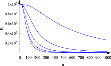
Figure 11. The decay of the number Kn of survivors with the number of bounces n (k = 0.75, j = 0.2) for radii of curvature (from top to bottom) r = 0.01, r = 0.05, r = 0.1, r = 0.15, and r = 0.2. The number of initial points is K0 = 106 uniformly distributed in x with v0 = 3.
Download figure:
Standard image High-resolution imageTable 1. The dependence of the escape rate κ and average lifetime  on the radius r of curvature.
| r | 0.01 | 0.05 | 0.1 | 0.15 | 0.2 |
| κ | 0.0014 ± 0.0001 | 0.0049 ± 0.0002 | 0.0086 ± 0.0006 | 0.0125 ± 0.0007 | 0.0161 ± 0.001 |

| 720 ± 50 | 204 ± 8 | 117 ± 8 | 80 ± 5 | 62 ± 4 |
The escape rate does not depend on the details of the initial distributions taken, it is a property of the system. Table 1 shows that the average lifetime falls below 100 by reaching r = 0.15.
The lack of long trajectories implies that the characterisation of chaos becomes less and less reliable as r increases. We have determined the phase space patterns and found similar results for larger r values as seen in figure 9 for r = 0.01. The average logarithmic distance between point pairs increases monotonically, indicating chaos for any r. The  graph looks similar to figure 8 up to r = 0.1, even the slope is nearly the same as for r = 0.01. For larger values of the radius, however, the graph becomes much more bent, and a linear fit can be applied to a rather short interval only, making the determination of a Lyapunov exponent unreliable.
6. The effect of velocity-dependent COR
Up to now, we have confirmed the statement that a ball's bouncing motion on rounded edge stairs is chaotic, at least within the framework of the model. The tricky feature found is that the motion with chaotic properties lasts for a finite number of bounces, but still much larger than what one can observe in real life. From a theoretical point of view, however, it can be of interest to investigate a modified model that incorporates a possibility of a (theoretically) unlimited number of bounces. To this order we turn to a formal extension by keeping the model's billiard character. In order to avoid, or at last weaken, the tendency of flying away we have to decelerate fast balls more than slower ones. This can be done by allowing COR to become velocity-dependent, with an overall decrease with the velocity. The literature discusses this effect in detail (see e.g. [13, 14]), we just choose a form convenient for our purposes here. Since the tangential COR proved to be able to weaken the tendency for an instability, we decide to make quantity j to be velocity-dependent, along the curvature only. We have experienced with different functions, but finally, the perhaps simplest form performed the best. The form phenomenologically taken is a simple exponential:

where v't is the tangential component of the impact velocity, and δ is a constant. Note that for small velocities (for v't ≪ 1/δ) the tangential COR is practically unity, as in the set-up investigated in section 4.1, but for v't = 1/δj falls down to 0.37, and for v't = 2/δ to j = 0.14. The application of relation (21) might be considered as a way to incorporate into a gravitational billiard the effect of air drag, a mechanism of velocity-dependent dissipation.
Our numerical simulations support that there is a range in parameter δ where the dynamics becomes practically permanently chaotic with this choice: the probability of any kind of escape is negligible. In addition, this is valid in the whole r range investigated, thus precise Lyapunov exponent values can be determined everywhere.
As an example we show the phase space patterns, representing a chaotic attractor in this case, in figure 12 with δ = 0.3. With this delta, the average of the velocity-dependent COR on the attractor comes to be around 0.27, a number close to the value j = 0.2 used in previous sections. To show the stability of this model, we have taken the largest radius considered, r = 0.2. The patterns are rather similar for all smaller values of r, and do not even depend much on whether v't in (21) is replaced by the normal component, or the modulus of the impact velocity.

Figure 12. The chaotic attractor in the two phase planes (v, x) (a) and (u, x) (b) in the case of a velocity-dependent tangential COR on the curvature, as given by (21) with δ = 0.3 for r = 0.2 and k = 0.75. Only the first 8000 points are displayed. The third panel exhibits a three-dimensional view of the attractor, with 20 000 points shown. Here, the positive direction of the x axis is to the left, in order to make the range 1 − r ⩽ x < 1 more conspicuous.
Download figure:
Standard image High-resolution image
Over the horizontal part of the step, for x < 1 − r, the pattern closely resembles the characteristics of the transient dynamics before escape takes place (cf figure 9), but over the curvature, 1 − r ⩽ x < 1, new features show up. Right around x = 1 − r there is a tendency of increase in u, but the shape remains bounded and the permitted u values appear to tend to nearly zero by the end of the step. Thanks to the strongly increasing dissipation with the velocity as expressed by (21), all u values remain below about 4, there is thus no need to apply any artificial threshold. In the vertical component a decreasing trend is visible for x > 1 − r which leads to slightly negative values at the end, representing nearly tangential impacts. To have an opportunity to see the attractor in the full phase space (x, u, v), too, panel (c) provides a spatial representation.
Problem 14. What is the explanation of the fact that the attractor points go down to nearly zero at about x = 1 − r in panel (b) of figure 12?
The real space paths remain similar to the one shown in panel (b) of figure 10, and the lack of escape makes the determination of Lyapunov exponents straightforward for any r. For each radius, the average was taken for approximately 105 pairs of trajectories on the attractor, with an initial distance of 10−11 between each other. The results are given in table 2. To estimate the reliability of the quantities, the errors are also given. All in all, the results indicate a pronounced chaos in all cases.
Table 2. The dependence of the Lyapunov exponent on the radius of curvature with δ = 0.3.
| r | 0.01 | 0.05 | 0.1 | 0.15 | 0.2 |
| λ | 0.195 ± 0.015 | 0.316 ± 0.016 | 0.480 ± 0.020 | 0.724 ± 0.026 | 0.862 ± 0.033 |
7. Summary
After a detailed study, we can say that the intuition of the authors of schoolbook [1] is correct, the motion of a ball bouncing down on stairs modelled as a gravitational billiard is unpredictable, provided the stair is not rectangular. Chaos, however, can only be classified properly if the motion is long-lasting, a few bounces do not suffice. It is because of this requirement that the analysis turns out to be more demanding than perhaps anticipated. When searching for such motions, we had to realise that the standard COR reducing the normal velocity component only is unable to prevent the ball from flying away, there is a tendency for unlimited acceleration in spite of this form of dissipation. This lead us to introduce a tangential COR, which along with the standard one, converts the motion to remain within the validity of the model over long periods of time. The (transiently) chaotic nature of the dynamics was possible to demonstrate, in fact, from the smallest possible radius on. The length of transient chaos turned out to be shrinking with increasing radii, making the statistics less reliable. This experience certainly shows that the transient form of chaos might be more generic than assumed, and it is worth being acquainted with the basics of this form of motion, too, along with the elements of how to investigate it. The permanent form of chaos was possible to find within the model only via introducing a velocity-dependent COR.
We think that the investigation presented here, or parts of it, can be used as undergraduate projects. The background is solely oblique projection and dissipative collision rules, the student, while working on the project, might nevertheless become familiar with the elements of chaos science, too.
Acknowledgments
We are grateful to G Homa, D Jánosi, Gy Károlyi, T Kovács, T Meszéna, and K Tóth for useful comments on the manuscript. Special thanks are due to A Schramek, the physics teacher of ÁT for motivating him for this project as a 10th grader, two years ago. We would like to thank B Tóth for the help he provided in the design of the webpage, and C S Kiss, Z Molnár, G Takács, I Stocker for their grammatical suggestions. This study was funded by the Content Pedagogy Research Program of the Hungarian Academy of Sciences and by the Hungarian NKFIH Office under Grant K-125171. The paper is dedicated to the memory of Márton Gruiz, the first author of the precursor paper [2], who called our attention to the challenges hidden in the phenomenon of bouncing on stairs.
Footnotes
- 4
Both the detailed solutions of the problems and the demo software are available on the website https://theorphys.elte.hu/fiztan/stairs.
- 5
An alternative approach is also possible: the first intersection point of the parabola arc representing the flight in vacuum with the shape of the staircase can always be found as a solution of a quartic equation. This might be solved numerically with the desired accuracy, then the time and velocity data can be determined afterwards. Our choice is motivated by the fact that the process is more similar this way to the one followed in the rectangular case in [2].
- 6
- 7
In the simplest model, the tangential COR can be related to the more standard normal COR. The force Fr,n (t) acting normally to the surface of contact during the nth collision sets the difference of the radial momentum: ∫Fr,n (t)dt = Δpr,n . If the positive direction is normally outward, as the direction of Fr,n , Δpr,n = m*(1 + k)v'r,n . Since, as one knows that Ff,n (t) = μFr,n (t), where μ is the coefficient of sliding friction, the two time integrals, and thus the momentum differences too, are proportional to each other. As a consequence, there is a linear relation between j and k but the coefficients, apart from μ, also depend slightly on the angle under which the ball hits the surface (see [19]).
- 8