


Abstract
The nonlinear behavior characterises a wide range of physical phenomena. Finding solutions that describe the behavior of nonlinear systems with respect to time is usually a challenging procedure. In addition, it is important to express the solutions using elementary functions so they can be easily applied in practical applications. In this paper, an interesting nonlinear oscillation was explored; the oscillation of a rigid sphere on an elastic half-space. A simple methodology based on the conservation of energy was used to find the position of the sphere with respect to time. The data was then fitted to appropriate functions that can be used to describe the behavior of the system with different levels of accuracy. It was found that a Fourier series function is an accurate, yet simple solution to describe the sphere's behavior. In addition, approximate expressions that relate the period of the motion with respect to the range of displacements was also presented.
Export citation and abstract BibTeX RIS
1. Introduction
Nonlinear oscillations can be found in a wide range of physical systems [1]. Extended research results have been published regarding the mathematical analysis of the complex behavior of nonlinear oscillators [1]. It is significant to mention that the scientific interest regarding the nonlinear behavior of physical systems remains undiminished up to date for research [2–13] or educational purposes [14–19]. However, the procedure to find the expressions that describe the behavior of nonlinear oscillators with respect to time is a challenging task. The basic goal when a nonlinear oscillation is explored is to find approximate solutions of the related differential equation in terms of elementary functions. Using this approach, the solution can be easily applied to practical applications.
In this paper an interesting nonlinear oscillator will be explored, the rigid sphere—elastic half-space system. An elastic half-space is an elastic material that extends infinitely in all directions including depth with the surface at the top to be considered as boundary [20]. The behavior of an elastic half-space is described by its Young's modulus and Poisson's ratio. Despite the fact that an elastic half-space is an ideal mathematical concept, it has been used in a wide range of applications from nanotechnology [21–24] and contact mechanics [25, 26] to seismics [27–30]. In fact, is a useful tool that can be used to represent the behavior of materials that have a linear elastic response [31]. Thus, it can be used as a mean to provide a useful insight in a significant number of physical phenomena in which elastic objects interact.
The problem to be studied in this paper is the nonlinear oscillation of a rigid sphere on an elastic half-space. The aforementioned motion is described by a second-order nonlinear ordinary differential equation that presents significant complexity [32]. In a previous publication, it was shown that for small displacements, the sphere's motion can be considered as harmonic [32]. However, in this paper, cases with significant displacement range will be explored. The basic goal of this paper is to find accurate solutions using elementary functions that describe the behavior of the aforementioned physical system. In addition, the relation of the motion's period with respect to the range of displacement will be explored. Towards this purpose, a simple method will be used that relies on the energy conservation principle. The approach presented in this paper is simple and can be used in post-graduate physics lectures to provide a methodology for the analysis of complicated non-linear phenomena.
2. The sphere's oscillation on the elastic half-space
Assume a rigid sphere with mass m that is placed at the surface of an elastic half-space. The system elastic half-space—sphere is placed at a constant gravitational field,  . At an arbitrary position the applied net force on the sphere equals to:

In equation (1),  is the applied force on the sphere by the elastic half-space and
  is the sphere's weight. According to the Hertz contact theory [32, 33],

In equation (2), F is the applied force, E* is the reduced modulus of the elastic half-space, R is the sphere's radius and y is the deformation of the surface from its initial position. The reduced modulus and the Young's modulus are connected by the following equation [32, 33]:

where E is the Young's modulus and v is the Poisson's ratio. At this point it must be noted that equation (2) is valid under the assumption that y ≪ R (i.e. the deformation of the surface is significantly smaller compared to the sphere's radius). A typical limit presented in the literature is y ⩽ 0.1R [21, 32, 33]. In addition, at the equilibrium position the deformation of the surface is y = yeq and the net force on the sphere is zero,

At an arbitrary position y = yeq + Δy, the differential equation that describes the sphere's motion is the following,

Equation (5) is a second-order nonlinear ordinary differential equation and as a result the sphere's motion is not harmonic. Free body diagrams for the equilibrium and an arbitrary position described respectively by equations (4) and (5) are also presented in figure 1.

Figure 1. Free body diagrams, equilibrium and non-equilibrium positions. The dashed line represents the level of the center mass of the sphere at each position.
Download figure:
Standard image High-resolution image3. The position of the sphere with respect to time function
To derive the y = f(t) function, the energy conservation principle will be applied. The range of the sphere's displacements is assumed to be 0 ⩽ y ⩽ y0, where y0 = 0.1R (i.e. according to the restriction that was presented in the introduction theory). The force applied on the sphere by the elastic half-space is conservative since  . As a result, F = −dUel/dy. In addition, using the work-energy theorem,

Hence, the potential energy of the elastic deformation (using also equation (2)) of the half-space can be calculated as below,

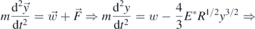
Thus, the energy conservation principle between the two positions as presented in figure 2 can be written as follows (assuming that at the initial position the sphere's velocity is zero, y-coordinate origin is at the undeformed surface and the y-axis is pointing down):
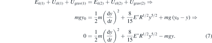

Figure 2. (a) The sphere at its initial position (the undeformed elastic half-space). The sphere's initial velocity is zero. At this position y = 0 and the potential energy of the elastic deformation of the half-space is also zero (Uel(1) = 0). The gravitational potential energy at y = 0 is Ugrav(1) = mgy0. (b) The sphere at an arbitrary position y. At this position Ugrav(2) = mg(y0 − y),  and
and  .
.
Download figure:
Standard image High-resolution imageUsing equation (7) it is derived that,
if y = 0, then  (as it was already mentioned).
In addition,  for y = y0. Thus, (using also equation (4)), it is concluded:

As a result, the position at which the net force is zero (equilibrium position) is not at y = y0/2. In addition, using equation (4), equation (7) can be written in the form,

By substituting equation (8) to (9), it can be derived,

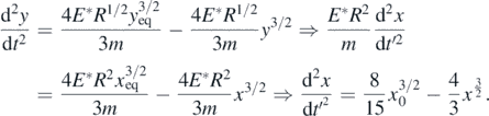
To facilitate the analysis the dimensionless parameter x will be used, where x = y/R. Thus,

Using, the transformation y = xR, equation (10) can be written in the form,
where

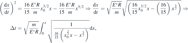
Or, assuming that, t0 = 0, Δt = t − t0 = t,

where,

The magnitude t' calculated by equation (13) is a dimensionless parameter that if it is multiplied with the factor  , it will provide the moment at which the sphere is at the arbitrary position y = xR. The solution of the integral provided by equation (13) is presented as follows,
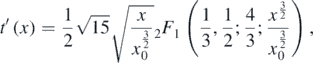
where, 2
 is the p = 2 and q = 1 generalised hypergeometric function. It must be also noted that the abovementioned function is only valid in the regime
  which is almost the complete domain 0 ⩽ x ⩽ x0 = 0.1. Although the aforementioned equation cannot be inverted, by tabulating
  , with x0 ∈ (0, 0.1) and plotting such list, the graph of the inverted function, i.e. of x = f(t') plot is presented in figure 3(a). Many functions were tested to fit the data. It was found that a Fourier series function, perfectly fits the data. More specifically, a function in the following form was used for data fitting,
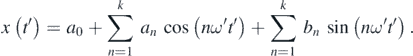

Figure 3. (a) The x with respect to t' data as calculated using equation (13) and the x = f(t') fitted curve (using a Fourier series function) at the domain 0 ⩽ t' ⩽ T'/2. (b) The y = f(t) data and the fitted curve at the same domain. The Fourier series function perfectly fits the data since the R-squared coefficient is equal to 1,  .
.
Download figure:
Standard image High-resolution imageUsing k = 2, the fit was perfect since the R-squared coefficient resulted equal to 1 ( . Thus, the x = f(t') is presented as follows:

In equation (14), a0 = 0.047 60, a1 = −0.049 99, b1 = −8.776 × 10⁻⁵, a2 = 0.002 408, b2 = −2.918 × 10⁻⁵, ω' = 0.6506.
The function that represents the position (y) with respect to time (t), y = f(t) can be then found (figure 3(b)),

where, 0 ⩽ t < ∞.
In equation (15), t is given by equation (12), and 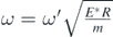 , (i.e. ω't' = ωt).
In addition, according to figure 3, at x = 0, t' = 0, while at x = 0.1, t' = 4.8288. The half-period of the motion (duration of the motion from the position y = 0 to the position y = y0) is equal to T/2, where 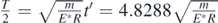 , thus
 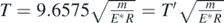 (where, T' = 9.6575).
However, in order to test if equation (15), accurately represents the position of the sphere with respect to time, it should be investigated whether the solution satisfies the second-order nonlinear ordinary differential equation, presented at section 2, (equation (5)). For this purpose, equation (5) was written as follows,
Thus, the functions,
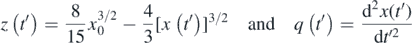
were plotted and compared (figure 4(a)). In particular,  function, was fitted to
  data in the domain 0 ⩽ t' ⩽ 5T'. The R-squared coefficient resulted 1, (
 . The same accuracy was presented for bigger domains as well (e.g. 0 ⩽ t' ⩽ 100T'). As a result, equation (15) is an accurate solution of equation (5). The position of the sphere with respect to time over the interval 0 ⩽ t ⩽ 5T is also presented in figure 4(b).

Figure 4. (a) q(t') and z(t') data is identical ( . Thus, equation (15) is an accurate solution of equation (5). (b) The position of the sphere with respect to time over the interval 0 ⩽ t ⩽ 5T.
Download figure:
Standard image High-resolution image4. Solutions for smaller range of displacements
In section 3 it was assumed that the initial position of the sphere (i.e. the position at t = 0) was y = 0. In this section, several other cases will be examined. If the elastic half-space is deformed when the sphere is at its initial position (i.e. y = yin at t = 0), then  and Ugrav(1) = mgy0. In addition, at an arbitrary position 2,
 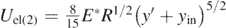 and
and  , where y' is the sphere's distance from its initial position yin and y0 the oscillation's range of displacements. In addition, it is assumed that Ek(1) = 0 and
 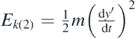 (figure 5). Thus, the conservation of energy principle can be written as follows:


Thus,  , where
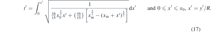
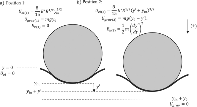
Figure 5. (a) The sphere at its initial position (position 1). The sphere's initial velocity is zero. At position 1 the potential energy of the elastic deformation of the half-space is  and the gravitational potential energy is Ugrav(1) = mgy0. (b) The sphere at an arbitrary position. At this position
  ,
,  and
and  .
.
Download figure:
Standard image High-resolution imageA numerical methodology was followed to derive the x' = f(t') function in each case. Briefly, multiple calculations of the integral as provided from equation (17) were performed as follows:


It was selected,  . Using the aforementioned integral (equation (17)) the x' = f(t') and the y = f(t) functions were determined (where y = y' + yin). In particular, the y = f(t) function was determined for 5 additional cases (for initial position equal to 0.01R, 0.02R, 0.03R, 0.04R and 0.05R, without initial velocity). In every case, the solution was in the form of equation (15). The fitting factors for each case are presented in table 1. In addition, the y = f(t) graphs for each case (included the case studied in section 3) are presented in figure 6. In every case
  (in the cases of section 4 there is also a correlation of m, E*, R in order to achieve that:
  ). In other words, we use 'the exact same sphere' on the 'exact same half-space'. The only difference is that the kinetic energy of the sphere at the equilibrium position in each case is smaller compared to the case of section 3. Thus, the range of displacements will be also smaller.
Table 1. Fitting factors for different initial positions of the sphere (for initial position equal to 0.01R, 0.02R 0.03R, 0.04R and 0.05R).
| yin (x R) | a0 | a1 | b1 | a2 | b2 | ω' |
|---|---|---|---|---|---|---|
| 0 | 0.047 60 | −0.049 99 | −8.776 × 10⁻⁵ | 0.002 408 | −2.918 × 10⁻⁵ | 0.6506 |
| 0.01 | 0.039 96 | −0.041 46 | −1.842 × 10⁻⁵ | 0.001 509 | −6.472 × 10⁻⁶ | 0.6631 |
| 0.02 | 0.031 71 | −0.032 59 | −5.3 × 10⁻⁶ | 0.000 8795 | −1.373 × 10⁻⁶ | 0.6714 |
| 0.03 | 0.022 99 | −0.023 43 | −8.341 × 10⁻⁷ | 0.000 4372 | −3.943 × 10⁻⁷ | 0.6771 |
| 0.04 | 0.013 84 | −0.013 99 | 8.73 × 10⁻⁷ | 0.000 1522 | −2.818 × 10⁻⁷ | 0.6807 |
| 0.05 | 0.004 274 | −0.004 281 | −3.374 × 10⁻⁵ | 6.979 × 10⁻⁶ | 1.203 × 10⁻⁵ | 0.6825 |
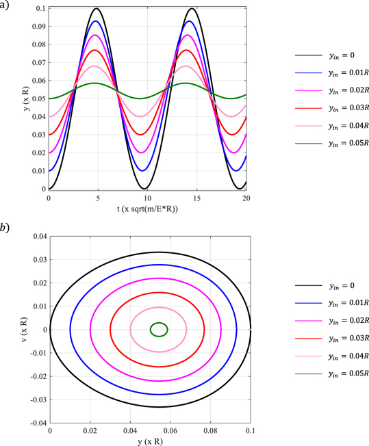
Figure 6. (a) The  functions for different initial positions. It can be clearly seen that there is a dependence of sphere's period from the range of displacements. (b) The phase diagram for each case presented in (a).
Download figure:
Standard image High-resolution imageUsing figure 6(a), it can be concluded that the period of the motion depends slightly on the range of displacements. In particular, there is a slight decrease in the period's motion as the range of displacements decreases. Additionally, in figure 6(b) the phase diagram for each case presented in figure 6(a) is shown.
5. The equation that provides the period of the motion
Several calculations of the motion's period with respect to the range of displacements were performed and presented in figure 7. It was assumed for every case that  . An exponential fit showed that the function T = f(y0) follows the exponential law:


Figure 7. (a) The period of the motion with respect to the range of displacements and an exponential fit (equation (18)). The R-squared coefficient resulted close to 1 ( ). (b) The exponential fitted curve provided by equation (18) (red line) and the period's values as resulted from equations (23) and (24). The two approaches provide similar results over the domain 0 ⩽ y ⩽ 0.025R. If y = 0.1R equations (23) and (24) provide 1.49% smaller value.
Download figure:
Standard image High-resolution imageFor very small amplitudes around the equilibrium position y = yeq (i.e. for very small range of displacements y0) it is concluded that  . However, this is the case of harmonic motion. The aforementioned statement can be easily proved using a Taylor's series expansion (keeping only the linear term):
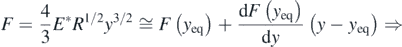

At an arbitrary position y, the differential equation that describes the sphere's motion is the following,

Using also equation (4) we conclude in:

In addition,  . Thus, the angular frequency in this case is
 ![$\omega =\sqrt{\frac{2{E}^{{\ast}}{R}^{\frac{1}{2}}{y}_{\mathrm{e}\mathrm{q}}^{\frac{1}{2}}}{m}}={y}_{\mathrm{e}\mathrm{q}}^{1/4}\sqrt{\frac{2{E}^{{\ast}}{R}^{\frac{1}{2}}}{m}}=\sqrt{2}{\left[0.1{\left(\frac{5}{2}\right)}^{-\frac{2}{3}}\right]}^{1/4}\sqrt{\frac{{E}^{{\ast}}R}{m}}=0.68\sqrt{\frac{{E}^{{\ast}}R}{m}}$](https://content.cld.iop.org/journals/0143-0807/42/2/025011/revision4/ejpabce1dieqn39.gif) , so the period of the motion is
, so the period of the motion is 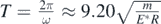 .
.
In addition, it has been also previously shown that for small displacements the sphere's motion can be considered as harmonic with period [32],

where r is the radius of the circle at contact depth (which is considered to be constant for very small displacements). Hence, assuming a very small displacement from the equilibrium position  , the radius of the circle at contact depth is approximately,

By substituting, equation (22) to (21), it can be easily concluded that  .
.
Equation (21) can be approximately used for any case, if the average radius at contact depth  is used,

The average radius at contact depth is determined as follows:

Equations (23) and (24) provide an accurate approach in the domain 0 ⩽ y0 ⩽ 0.025R. If y0 = 0.1R the aforementioned approach leads to 1.49% lower value regarding the motion's period. However, equations (23) and (24) provide the physical significance of the exponential law presented by equation (18). In particular, the term  can be considered as the 'average stiffness' of the system. For small oscillations over the position
  , the radius at contact depth is
  . If the oscillation's range of displacements increases it can be easily shown that
  , and as a result the period is greater compared to the previous value. This fact explains the period's increase with the increase of the range of displacements.
In addition, an interesting question also arises; how small the range of displacements should be in order to consider the motion as harmonic? According to equation (19),
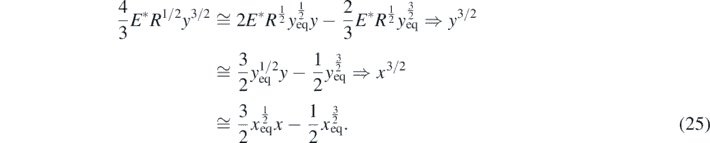
In equation (25), 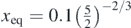 and 0 ⩽ x ⩽ 0.1. Equation (25) is valid for a small range of displacements around xeq. To find 'how small' the range of displacements should be a graphical representation of the functions
  and
and  is presented in figure 8(a). In addition, the function
  is also presented in figure 8(b). The harmonic motion approximation is valid for
  . According to figure 8(c), a rational approximation should be:


Figure 8. (a) The f(x) and the g(x) functions. For a small range around xeq these functions provide similar results. (b) The  function. The sphere's motion can be considered as harmonic for h(x) → 0. (c) At the domain 0.0539 ⩽ x ⩽ 0.0547, h(x) ≅ 0.
Download figure:
Standard image High-resolution imageIn other words, the sphere's initial position should be yin = 0.0539R. In this case the sphere's motion can be accurately considered as harmonic.
6. An alternative approximate solution
As an alternative approximate solution of equation (5) (in terms of the range of sphere's displacements) the following function can be used,

In particular, equation (26) was fitted to the y versus t data for the case of y0 = 0.1R and yin = 0 and n resulted in 2.271 (in addition, ω' = 0.6506, since also in this case ωt = ω't'). Furthermore, the R-squared coefficient resulted in  . Thus, equation (26) can be considered as an acceptable approximate solution. Equation (26) does not provide the accuracy of equation (15) (see figure 9), however it has the significant advantage that it is expressed in terms of the range of displacements (y0) in each case. In addition, it reveals that y ⩾ 0 in every case. Thus, the only unknown parameter that must be determined is the exponential factor n. Equation (26) was also tested for cases with smaller range of displacement and the results are presented in figure 10. In every case, ωt = ω't' (see also table 1). As it can be clearly seen, equation (26) can be better applied for a range of displacements within the domain 0.28R ⩽ y ⩽ 0.65R. However, it also provides acceptable solutions for the other cases. An interesting fact to be noted is that the range of values of n parameter was in a relatively small range 2.090 ⩽ n ⩽ 2.271 for all the examined cases.
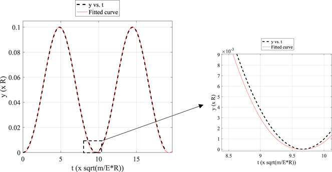
Figure 9. An alternative fitting (equation (26)) to the data. Equation (26) provides an acceptable solution for differential equation (5), however, it does not perfectly 'match' to the data for every moment of the motion.
Download figure:
Standard image High-resolution image
Figure 10. (a)–(e) Fitting equation (26) to the numerical data for 5 cases (the same cases as presented in table 1 and figure 6 for initial position equal to 0.01R, 0.02R, 0.03R, 0.04R, 0.05R) with significantly different range of displacements. (f) The y = f(t) function for the cases presented in images (a)–(e).
Download figure:
Standard image High-resolution image
7. Discussion
In this paper, the nonlinear oscillation of a rigid sphere on an elastic half-space was explored. It was proven that a Fourier series expansion as provided by equation (15) is an accurate solution of differential equation (5) and can be used to provide the sphere's position with respect to time for different range of displacements around the equilibrium position. In addition, an approximate solution (equation (26)) that is expressed in terms of the range of displacements can be also used. A significant result that was proven by the presented analysis is that the period of the motion depends on the range of displacements (figures 6(a) and 7(a)). However, for small displacements around the equilibrium position the motion's period becomes constant,

and as a result, the motion can be considered as harmonic. At this point it should be noted that the most typical result arising from the harmonic oscillator is that the period is independent of the amplitude of the oscillation. The aforementioned nonlinear behavior, that becomes linear for small displacements range, is similar to the simple pendulum case. More specifically, when dealing with large oscillations, the complete period of a pendulum is given by an expansion in power series of the initial angle at which the pendulum is dropped [34],

In addition, in the presented by this paper case, using a Taylor's series expansion of equation (18) and assuming that the equilibrium position is at y = 0 it is concluded:

Thus, in this case the complete period of the sphere's motion on the elastic half-space is given by an expansion in power series of the motion's range of displacement. In addition, as it is obvious from the aforementioned Taylor's series expansion, for small values of y0,  (the case of harmonic motion as it has been already mentioned).
It must be also noted that the analysis presented in this paper can be also applied in other cases of applying forces that are not proportional to the body's displacement (forces of the several form F = cyu ). In the above-mentioned cases the resulting differential equation to be solved has the form y'' = mg − cyu . Those are the cases of forces applied by non-linear springs, by liquids (when a rigid body is partially skunked into the liquid), by half-spaces on rigid bodies (with different geometries), by elastic membranes etc. Thus, future work will focus on the equations of motion that describe the aforementioned cases.
8. Conclusion
In this paper the nonlinear oscillation of a rigid sphere on an elastic half-space was explored. It was found that a Fourier series function (using two sinusoidal and two cosinusoidal terms terms) perfectly fits to the data of the position of the sphere with respect to time. Moreover, as an additional approximate solution, a function in terms of the range of displacement was also provided. Special attention was given to find solutions in terms of elementary functions in order for the solutions to be easily applied in relative applications. It was also shown that the oscillation's period depends on the range of displacements with an exponential law. In particular, if the range of displacements increases, the period of the motion increases since the average stiffness of the system decreases.
The presented by this paper results are similar to the ones of the oscillation of the simple pendulum. In particular, in both cases, the period of the motion can be described by a power series in terms of the range of displacement and for small oscillation's amplitudes the motion can be considered as harmonic.