

Abstract
This paper discusses the oscillations of a spring (slinky) under its own weight. A discrete model, describing the slinky by N springs and N masses, is introduced and compared to a continuous treatment. One interesting result is that the upper part of the slinky performs a triangular oscillation whereas the bottom part performs an almost harmonic oscillation if the slinky starts with 'natural' initial conditions, where the spring is just pushed further up from its rest position under gravity and then released. It is also shown that the period of the oscillation is simply given by  , where L is the length of the slinky under its own weight and g the acceleration of gravity, independent of the other properties of the spring.
Export citation and abstract BibTeX RIS

Original content from this work may be used under the terms of the Creative Commons Attribution 4.0 licence. Any further distribution of this work must maintain attribution to the author(s) and the title of the work, journal citation and DOI.
1. Introduction
A slinky, invented in the 1940 by Richard James, is in the context of this paper a spring that oscillates under its own weight without any additional mass attached to it with a quality factor high enough to observe the oscillations, see figure 1. There are many articles on a falling slinky [1–3] and the suspended slinky [4–6]. This article studies interesting new aspects of an oscillating suspended slinky. A new aspect, derived in this article, is that the upper and lower part of a slinky show different oscillation patterns, a triangular versus an almost harmonic oscillation motion, respectively. These mathematical findings can easily be verified experimentally using in addition to the slinky only a smart phone to record the oscillations and open source software to analyze the motion. On the theoretical side students will apply their knowledge in solving a system of differential equations and the wave equation with given initial conditions. Undergraduate level of mathematics and physics is required.

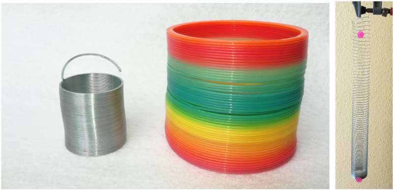
Figure 1. Left: photograph of the two slinkies used in the experiments. Right: the experimental setup using the metal slinky with two marks used to track the oscillations.
Download figure:
Standard image High-resolution imageThe article is organized as follows. Equations of motion are derived and solved for the discrete case where the slinky is described by N masses and springs in section 2. Section 3 treats the continuous case. Section 4 compares the results obtained analytically to experimental results.
2. Discrete case
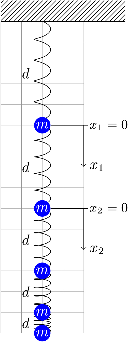
The slinky is modeled by N identical massless springs with spring constant d and masses m in between as shown in figure 2. A given mass experiences forces from the two neighboring springs leading to the following equation of motion

where the xj denotes the excursion from the rest position of the mass. An exception is the first and last spring. In this case the equations of motion read


This results in the following system of coupled differential equations

with

and


Figure 2. Slinky modeled by N masses and N springs. The picture shows the rest position under its own weight.
Download figure:
Standard image High-resolution imageIn contrast to the corresponding matrix of a falling slinky [3], there is a 2 in the upper left corner instead of a 1. This is because the upper mass of the suspended slinky experiences a force from two springs, whereas in the case of the falling slinky the upper mass is only experiencing a force from one spring.
A solution with initial condition  is:
is:

Inserting equation (7) into equation (4) leads to the eigenvalue problem

The general solution of equation (4) is thus

where  are the square roots of the eigenvalues and
a
j
the corresponding eigenvectors. For a given initial condition
x
(0) =
x
0, the vector
c
is determined by inverting
are the square roots of the eigenvalues and
a
j
the corresponding eigenvectors. For a given initial condition
x
(0) =
x
0, the vector
c
is determined by inverting

where A is the matrix with the eigenvectors as columns.
We assume the springs to be massless and of zero length when not exposed to a force. Then the rest position of the first (top) mass is given by

The first spring is stretched by all N masses. The second spring is accordingly stretched by N − 1 masses. This leads to

The position of the Nth mass is thus

To study oscillations we just pull (push) the slinky further down (up) from its rest position. The initial condition (deviation from x rest) is given by

For the first and last mass from top one finds:
Now that the initial conditions are fixed, one can calculate the oscillations using equation (9). Figure 3 shows the results for the parameters given in table 1. The amplitudes are the larger the lower the position along the slinky. At the top, the oscillations have a triangular shape whereas at the bottom the oscillation is more sinusoidal.
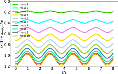
Figure 3. Oscillations as a function of time t for the different masses. The dashed lines for the top and bottom mass are results from the treatment of the continuous case (section 3). They perfectly coincide with the solution for the discrete case.
Download figure:
Standard image High-resolution imageTable 1. Parameters for oscillations shown in figure 3.
| Parameter | Value | Meaning |
|---|---|---|
| N | 10 | Number of masses |
| X0/m | 0.1 | Deviation from rest position for bottom mass |
| D/kg s−2 | 0.15 | Spring constant of slinky |
| d = ND/kg s−2 | 1.5 | Corresponding spring constant of single spring between |
| two masses in figure 2 | ||
| M/g | 30 | Mass of slinky |
To understand this behavior in more detail, we consider in the next section a continuous distribution of the mass along the slinky. This is a typical approach in physics. One starts to study oscillations of a single mass, the next step is to look at coupled oscillation of N = 2, 3, ... masses, as we did in the present section, finally going to N = ∞, which corresponds to the continuous case.
3. Continuous case
If N → ∞ and m → 0 such that Nm = M remains constant, one reaches a continuous mass distribution. This system can best be described by a dimensionless variable n which is defined by the turn number of the spring divided by the total number of turns, i.e. 0 ⩽ n ⩽ 1 [5]. The position x as a function of n along the slinky under gravity can be derived from the following consideration. Under gravity the stretching x(n + dn) − x(n) of the slinky is proportional to the remaining mass below the position n. Since this mass is proportional to (1 − n), one finds:

This leads to

normalized such that the total length is x(1) = L. Inverting equation (16) leads to

Appendix A shows in detail that, using n instead of the vertical position x as a coordinate, the system can be described by the following wave equation [5, 7]

where a wave is propagating with constant velocity  . This is not the case if the coordinate x is used instead of n. s(n, t) is the deviation of the slinky from its rest position as a function of the relative turn number n and time t.
If we pull the slinky at the bottom, according to equation (16) the initial conditions are given by

where X0 denotes the excursion of the bottom of the slinky from its rest position. Further initial and boundary conditions are


Equation (22) assures an anti-node at the open end n = 1.
The solution is given by

To fulfill condition equation (22), we have

Finally equation (18) leads to:

The fundamental angular frequency is thus given by
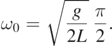
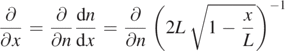
For the period length of the oscillation one finds

independent of the mass or other properties of the slinky. This result has been derived in [5] in a different context as a round trip time of a pulse.
The length L under its own weight is easily derived from equation (13)

Note that d is the spring constant of a single spring (see figure 2). The spring constant of the entire spring is D = d/N. The dependence of the period duration T on M and D is hidden in the length L(M, D). T can also be expressed as

For the parameters given in table 1, one finds ω0 = 3.49 s−1 which is very close to the solution found in the discrete case for N = 10, ω0,N=10 = 3.34 s−1. Figure 4 shows a comparison of the frequencies for various values of N for the first three contributing frequencies.
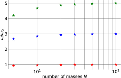
Figure 4. First three frequencies for N = 5, 10, 20, 30, 50, 100 divided by the fundamental frequency ω0 for the continuous case.
Download figure:
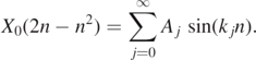
Standard image High-resolution imageThe coefficients Ai in equation (23) are found by a Fourier analysis. As shown in detail in B, in order to satisfy the initial condition equation (19), one finds
The amplitude of the different frequencies is given by the factors Aj sin(kj n) in equation (23). At small n, i.e. at the top of the spring, one finds
The amplitudes have the ratios 1:9:25:...for j = 0, 1, 2, ... which corresponds to a triangular shape as observed in figure 3. At the bottom end of the slinky, i.e. n = 1 one has sin(kj n) = 1 resulting in


which almost corresponds to a pure sine wave. But even in the limit N → ∞ the bottom mass oscillation is not purely harmonic.
In figure 3 the dotted lines for the top and bottom mass show the solution (at n = 0.1 and n = 1 respectively) from the wave equation which agrees perfectly with the discrete solution with N = 10.
4. Comparison to experiment
Two slinkies (see figure 1 and table 2) were used to confirm equation (26) and to verify the motion of the top and bottom mass. Figure 5 shows a comparison of the measured and calculated period duration. A reasonable agreement is found.
Table 2. Parameters of slinkies used in experiments.
| Plastic | Metal | |
|---|---|---|
| nb. of turns | 52 | 93 |
| Mass M/g | 65 | 35 |
| Length L/m under gravity | 2.40 | 0.32 |
| Unstretched length L0/m | 0.07 | 0.04 |
| Diameter in cm | 7.8 | 3.5 |
Table 3. Results of the measurements with the two slinkies. L0 is the length in the unstretched state. The numbers in parentheses indicate the uncertainties. Ttheo was calculated using equation (26) with L − L0 as length.
| Length L/m | Length L0/m | Tmeas/s | Ttheo/s | |
|---|---|---|---|---|
| 2.400(5) | 0.070(2) | 2.50(2) | 2.757(1) | Plastic |
| 1.000(5) | 0.040(2) | 1.65(2) | 1.770(2) | Plastic |
| 0.440(5) | 0.028(2) | 1.11(2) | 1.152(3) | Plastic |
| 0.210(5) | 0.020(2) | 0.77(2) | 0.787(5) | Plastic |
| 0.100(5) | 0.010(2) | 0.50(2) | 0.542(7) | Plastic |
| 0.325(5) | 0.040(2) | 1.09(2) | 0.973(4) | Metal |
| 0.174(5) | 0.027(2) | 0.80(2) | 0.692(5) | Metal |
| 0.100(5) | 0.020(2) | 0.61(2) | 0.511(6) | Metal |
| 0.029(5) | 0.006(2) | 0.32(2) | 0.274(12) | Metal |
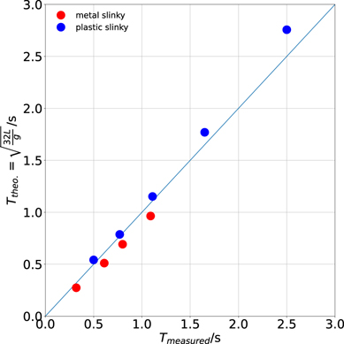
Figure 5. The calculated period length (equation (26)) vs the measured period length. The data are shown in table 3.
Download figure:
Standard image High-resolution imageFigure 6 shows the measurement of an oscillating slinky. The top plots are the oscillations and frequencies of a point at the top of the slinky, the bottom plots are the corresponding plots for the bottom end of the slinky. Qualitatively one observes the behavior in figure 3. The oscillation of the top point is more triangular shaped. It is worthwhile to mention that in these experiments it is important to pull or push the slinky from the bottom to have the correct initial conditions. If the slinky is for instance pulled at n ≈ 0.4, the oscillations look very different. In principle this could be studied by choosing the corresponding initial conditions in equations (10) or (19). This can also be seen as an invitation to perform more experiments with different initial conditions and compare them to the analytic solution.
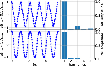
Figure 6. Left: oscillation of top and bottom part of the slinky. Right: the corresponding frequency spectrum.
Download figure:
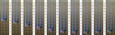
Standard image High-resolution imageThe points of figure 6 were obtained using the open source opencv library [8] which allows one easily to track a point in a video according to its color. The videos were taken using an ordinary smart phone. Figure 7 shows the analysis of ten video frames, where a point at the bottom of the slinky is tracked.
Figure 7. Analysis of ten video frames using the opencv library [8] to track a point at the bottom of the slinky. The result of the tracking is indicated by the green lines around the colored area. The images are taken 0.033 s apart.
Download figure:
Standard image High-resolution image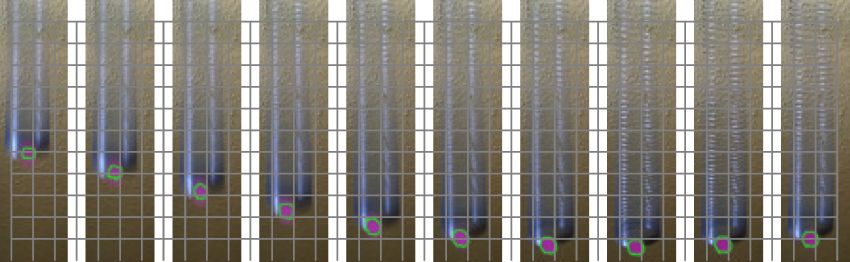
5. Summary and conclusions
Starting from discrete treatment with N masses attached to N springs the vertical motion of a suspended slinky was studied. A first observation of the discrete treatment is that the top part of the slinky performs triangular motions whereas the bottom part is more sinusoidal. Using a continuous model this could also be confirmed analytically. Measurements show a good agreement with the analytic results derived. The experimental results shown can by reproduced by students using only modest resources.
Acknowledgments
I would like to thank J Barth for comments and suggestions on the paper.
Appendix A.: Derivation of the wave equation
The wave equation for a string subject to a force F along the longitudinal direction reads

where ρ is the density and A the cross-sectional area of the string.
The force at a given n is given by

where M is the total mass of the slinky.
From equations (16) and (A.2) we can express the force and the density ρ as a function of the position x.


This leads to

As in references [5, 7] it is easier to write the wave equation in terms of the turn number n

Using
and dropping the tilde on s, the wave equation becomes

In terms of the relative turn number n the velocity  is constant.
Appendix B.: Determination of coefficients Ai
Equations (19) and (23) for t = 0 read
For j = 0 the sine term performs only one quarter of an oscillation between n = 0 and n = 1. Therefore the following integral is only evaluated over a quarter period length up to λ/4. To get the correct normalization the result has to be multiplied by 4. This results in the following expression for the Fourier coefficients Ai :

with λ = 2π/k0.