Did Schrödinger have other options?

The Schrödinger equation is the most famous equation in quantum mechanics [1–5]. In 1926, Erwin Schrödinger published his now famous equation and showed how to describe hydrogen-like atoms using it [6]. However, it is now known that while looking for the right equation, Schrödinger first explored, but did not publish, the equation that we today call the Klein–Gordon equation, which was first published also in 1926 by Oskar Klein and Walter Gordon [7, 8]. Schrödinger was well-aware of the Einstein's special theory of relativity [9]; thus, he knew that a relativistic quantum mechanics cannot be based on the Schrödinger equation because it is Galilean invariant [10, 11]. Schrödinger considered the Klein–Gordon equation because it is Lorentz invariant, thus valid for any two observers moving respect to each other at constant velocity [7–9]. Two weakness result from the Galilean invariance of the Schrödinger equation; first, two such observers will only agree in the adequacy of the Schrödinger equation, for describing the movement of a quantum particle, when the relative speeds between the observers is much smaller than the speed of the light in vacuum (c). However, this is not a big deal because we move much slower than the light. The second limitation of the Schrödinger equation is that it describes a particle with mass (m), with linear momentum (p) and kinetic energy (K) related by the classical relation K = p²/(2m), which is not valid at relativistic speeds [7–9]. Nevertheless, wave mechanics triumphed when Schrödinger, using the equation chosen by him, was able to reproduce the results previously obtained by Bohr for the energies of the bound states of the electron in the hydrogen atom [1–5]. This was possible because the electron in the hydrogen atom has non-relativistic energies [1–5]. Rigorously, the number of particles may not be constant in a fully relativistic quantum theory [7, 8]. This is because when the sum of the kinetic and the potential (U) energy of a particle with mass m doubles the energy associate to the mass of the particle, i.e. Ę = K + U = 2mc², then a pair particle-antiparticle could be created from Ę. Consequently, the number of particles is constant when Ę = K + U < 2mc². This is what happens in atoms and molecules; thus, this explains why the results obtained using the Schrödinger equation are a good first approximation in chemistry applications [5].

In between the Galilean invariant Schrödinger equation and the fully relativistic quantum mechanics, there is a quasi-relativistic energy region where Ę < 2mc² but Ę is so large that it is necessary to use an equation that describes a particle having a relativistic relation between p and K. It is then argued in this work that there is an intermediate option between the one chosen by Schrödinger (the equation named after him) and the one discarded by him (the Klein–Gordon equation). This third option, which is valid in the quasi-relativistic energy region, is the following quasi-relativistic wave equation [11–13]:

$$\begin{equation}\mathit{i}\hslash \frac{\partial }{\partial \mathit{t}}\psi =-\frac{{\hslash }^{2}}{\left({\gamma }_{\mathit{V}}+1\right)\mathit{m}}{\nabla }^{2}\psi +\mathit{U}\psi .\end{equation} \tag{ 1 }$$

In equation (1), ℏ is the Plank constant (h) divided by 2π, and γ_V a relativistic parameter depending on the square of the particle speed (V²) [9]:

$$\begin{equation}{\gamma }_{V}=\frac{1}{\sqrt{1-\frac{{V}^{2}}{{c}^{2}}}}.\end{equation} \tag{ 2 }$$

There is a striking similarity between the quasi-relativistic wave equation explored here (equation (1)) and the Schrödinger equation [1–5]. In fact, γ_V ∼ 1 when V ≪ c; therefore, equation (1) coincides with the Schrödinger equation at low particle speeds. While equation (1) is Galilean invariant for observers traveling at low speeds (V_o ≪ c) respect to each other [11], equation (1) describes a particle with mass which linear momentum and kinetic energy are related by the correct relativistic relation [11–13]. Consequently, while wondering about what would have done Schrödinger if he would have encountered this equation, the author of this work embarked in the exciting task of recreating the foundational times of wave mechanics. Facilitated by the similitude between the quasi-relativistic wave equation (equation (1)) and the Schrödinger equation, several interesting things have been found. First, a positive probability density can be defined for the solutions of quasi-relativistic wave equation [11]. Second, it has been possible to solve equation (1) in the context of several problems often included in introductory courses of quantum mechanics [11–13]; moreover, this has been done with no more difficulties than the ones encountered when solving the Schrödinger equation in the same context [1–5]. Third, a repetition of the Schrödinger success was achieved when using equation (1) for describing hydrogen-like atoms [13]. It was found that the exact solutions of this equation include the relativistic correction to the energies found using the Schrödinger equation [13]. This relativistic correction is traditionally calculated as a first order approximation using a perturbation theory [4, 14]. This suggests that the quasi-relativistic wave equation explored here could have been the foundational equation of quantum mechanics. Moreover, this equation could be used today for finding quasi-relativistic solutions of several practical problems, and for introducing the students to the intricacies of relativistic quantum mechanics without a notable complication of the involved mathematical techniques. In what follows, first, a brief summary of previous results is presented in section 2, then some of their consequences are discussed in section 3. Finally, the conclusions of this work are given in the last section.

When the speed (V) of a free particle with mass m is much smaller than the c, then the classical relation between K and p is given by the following relations [1–5]:

$$\begin{equation}K=\frac{{p}^{2}}{2m},\quad p=mV.\end{equation} \tag{ 3 }$$

In quantum mechanics, one can formally substitute K and p in equation (3) by the following energy and momentum quantum operators [1–4]:

$$\begin{equation}\hat{E}=\hat{K}=i\hslash \frac{\partial }{\partial t},\quad \hat{p}=-i\hslash \frac{\partial }{\partial x}.\end{equation} \tag{ 4 }$$

Then resulting the 1D Schrödinger equation for a free quantum particle with mass m [1–5]:

$$\begin{equation}i\hslash \frac{\partial }{\partial t}{\psi }_{\mathrm{S}\mathrm{c}\mathrm{h}}\left(x,t\right)=-\frac{{\hslash }^{2}}{2m}\frac{{\partial }^{2}}{\partial {x}^{2}}{\psi }_{\mathrm{S}\mathrm{c}\mathrm{h}}\left(x,t\right).\end{equation} \tag{ 5 }$$

However, equation (3) does not give the correct relation between K and p when the particle moves at faster speeds. Correspondingly, the Schrödinger equation (equation (5)) is not Lorentz invariant but Galileo invariant [10, 11]; thus, only should be used for slowly moving particles. At larger particle's speed, one should use the following well-known relativistic relations [9]:

$$\begin{equation}{E}^{2}-{m}^{2}{c}^{4}={p}^{2}{c}^{2}{\Leftrightarrow}\left(E+m{c}^{2}\right)\left(E-m{c}^{2}\right)={p}^{2}{c}^{2}.\end{equation} \tag{ 6 }$$

And

$$\begin{equation}E={\gamma }_{V}m{c}^{2},\quad p={\gamma }_{V}mV,\quad E=K+m{c}^{2}.\end{equation} \tag{ 7 }$$

One can then formally proceed as it is done for obtaining the 1D Schrödinger equation, and use equation (4) for assigning the temporal partial derivative operator to E in the first expression of equation (6) [7, 8, 11]. In this way, one can formally obtain the 1D Klein–Gordon equation [7, 8]:

$$\begin{equation}\frac{1}{{c}^{2}}\frac{{\partial }^{2}}{\partial {t}^{2}}{\psi }_{\mathrm{K}\mathrm{G}}\left(x,t\right)=\frac{{\partial }^{2}}{\partial {x}^{2}}{\psi }_{\mathrm{K}\mathrm{G}}\left(x,t\right)-\frac{{m}^{2}{c}^{2}}{{\hslash }^{2}}{\psi }_{\mathrm{K}\mathrm{G}}\left(x,t\right).\end{equation} \tag{ 8 }$$

The Klein–Gordon equation is Lorentz invariant and describes a free quantum particle with mass m and spin-0 [7, 8]. In contrast to the Schrödinger equation, a second-order temporal derivative is present in equation (8). This determines that equation (8) has solutions with positive and negative energy values while equation (5) has only solutions with positive energies, which is in correspondence with K having only positive values in equation (3) but E having positive and negative values in equation (6). The factor (E + mc²) is always different than zero for E > 0; consequently, equation (6) and the following algebraic equation are equivalents for E > 0:

$$\begin{equation}\left(E-m{c}^{2}\right)=\frac{{p}^{2}}{\left({\gamma }_{V}+1\right)m}.\end{equation} \tag{ 9 }$$

Each member of equation (9) is just a different expression of the relativistic kinetic energy of the particle [11]. Assigning the temporal partial derivative operator in equation (4) to E in equation (9) results in the following differential equation [12]:

$$\begin{equation}i\hslash \frac{\partial }{\partial t}{\psi }_{\mathrm{K}\mathrm{G}+}\left(x,t\right)=-\frac{{\hslash }^{2}}{\left({\gamma }_{V}+1\right)m}\frac{{\partial }^{2}}{\partial {x}^{2}}{\psi }_{\mathrm{K}\mathrm{G}+}\left(x,t\right)+m{c}^{2}{\psi }_{\mathrm{K}\mathrm{G}+}\left(x,t\right).\end{equation} \tag{ 10 }$$

A simple substitution in equations (8) and (10) shows that the following plane wave is a solution of both equations for E > 0:

$$\begin{equation}{\psi }_{\mathrm{K}\mathrm{G}+}\left(x,t\right)={\mathrm{e}}^{\frac{\mathrm{i}}{\hslash }\left(px-Et\right)}.\end{equation} \tag{ 11 }$$

The plane wave ψ_KG+ has an unphysical phase velocity equal to c²/V > c [11, 12]. However, one can look for a solution of equation (10) of the following form:

$$\begin{equation}\psi \left(\mathit{x},\mathit{t}\right)={\psi }_{\mathrm{K}\mathrm{G}+}{\mathrm{e}}^{\mathrm{i}{w}_{m}t},\quad {\mathrm{w}}_{\mathit{m}}=\frac{\mathit{m}{\mathit{c}}^{2}}{\hslash }.\end{equation} \tag{ 12 }$$

Such that ψ has a phase velocity smaller than c [11, 12]; thus

$$\begin{equation}\psi \left(x,t\right)={\mathrm{e}}^{\frac{\mathrm{i}}{\hslash }\left(px-Kt\right)}.\end{equation} \tag{ 13 }$$

Substituting ψ given by equation (12) in equation (10) results in the 1D quasi-relativistic wave equation for a free quantum particle with mass m and spin-0 [11–13]:

$$\begin{equation}i\hslash \frac{\partial }{\partial t}\psi \left(x,t\right)=-\frac{{\hslash }^{2}}{\left({\gamma }_{V}+1\right)m}\frac{{\partial }^{2}}{\partial {x}^{2}}\psi \left(x,t\right).\end{equation} \tag{ 14 }$$

Clearly, equation (14) coincides with equation (5) at low particle's speeds. Moreover, like for the Schrödinger equation, a positive probability density can be defined for the solutions of equation (14), which is Galilean invariant for observers traveling at low speeds respect to each other [11]. Despite this, equation (14) can be used for obtaining precise solutions of very interesting quantum problems at quasi-relativistic energies [11, 12]. At these energies, a particle moves so fast that the relation between p and K is relativistic; however, the number of particles remains constant because the particle does not move too fast. When the particle moves through a 1D piecewise constant potential U(x), equation (14) should be generalized in the following way [12, 13]:

$$\begin{equation}i\hslash \frac{\partial }{\partial t}\psi \left(x,t\right)=-\frac{{\hslash }^{2}}{\left[{\gamma }_{V}\left(x\right)+1\right]m}\frac{{\partial }^{2}}{\partial {x}^{2}}\psi \left(x,t\right)+U\left(x\right)\psi \left(x,t\right).\end{equation} \tag{ 15 }$$

Often, one looks for solutions of equation (15) corresponding to a constant value of the energy Ę = K + U = E + U – mc². However, K, γ_V and V² have a discontinuity wherever U(x) has one. Consequently, γ_V is a function of x in equation (15) because, in general, the square of the particle's speed (V²) depends on the position [12]. Nevertheless, for 1D piecewise constant potentials, one can look for a solution of equation (15) with the following form in each of the regions where K, γ_V, and V² are constants [1–4, 12, 13]:

$$\begin{equation}\psi \left(x,t\right)={X}_{K}\left(x\right){\mathrm{e}}^{-\frac{\mathrm{i}}{\hslash }\mathrm{E}t},\quad \it{\unicode{280}}=K+U.\end{equation} \tag{ 16 }$$

In equation (16), X_K is a solution of the following equation [1–4, 12, 13]:

$$\begin{equation}\frac{{\mathrm{d}}^{2}}{\mathrm{d}{x}^{2}}{X}_{K}\left(x\right)+{\kappa }^{2}{X}_{K}\left(x\right)=0,\quad \kappa =\frac{p}{\hslash }.\end{equation} \tag{ 17 }$$

And [12, 13]:

$$\begin{equation}\kappa =\frac{p}{\hslash }=\frac{1}{\hslash }\sqrt{\left({\gamma }_{V}+1\right)mK}=\frac{1}{\hslash }\sqrt{\left({\gamma }_{V}+1\right)m\left(E-U\right)}.\end{equation} \tag{ 18 }$$

The allowed values of κ are determined from equation (17) and the boundary conditions. Therefore [12]:

$$\begin{equation}K=\frac{{\hslash }^{2}{\kappa }^{2}}{\left({\gamma }_{V}+1\right)m}.\end{equation} \tag{ 19 }$$

As expected, when γ_V ∼ 1, equation (19) gives the non-relativistic values of the particle's energies at low speeds, K ∼ ℏ²κ²/(2m) [1–4]. Moreover, from equation (19) and the relativistic equation, K = (γ_V − 1) mc², follows that [12, 13]

$$\begin{equation}{{\gamma }_{V}}^{2}=1+{\left(\frac{{\lambda }_{\mathrm{C}}}{\lambda }\right)}^{2},\quad {\lambda }_{\mathrm{C}}=\frac{h}{mc},\enspace \lambda =\frac{2\pi }{\kappa }.\end{equation} \tag{ 20 }$$

In equation (20), λ_C is the Compton wavelength associate to the mass of the particle [7, 9], and λ is the de Broglie wavelength associated to p [1–4]. An analytical expression of the precise quasi-relativistic kinetic energy of the particle can then be obtained by substituting equation (20) in equation (19) [13]:

$$\begin{equation}K=\frac{{\hslash }^{2}{\kappa }^{2}}{\left[1+\sqrt{1+{\left(\frac{{\lambda }_{\mathrm{C}}}{\lambda }\right)}^{2}}\right]m}.\end{equation} \tag{ 21 }$$

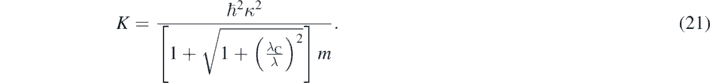
As expected, equation (21) match the non-relativistic expression of the particle's kinetic energy when p = h/λ is very small because λ ≫ λ_C. However, in each region where the value of U is constant, the values of K and then Ę = K + U calculated using equation (21) are smaller than the ones calculated using the Schrödinger equation. Several 1D problems have been solved using equation (15) including the 1D infinite rectangular well [11], the quantum rotor [11], reflection in a potential step [12], tunneling through a barrier [12], and bound states in a rectangular well [12]. The tridimensional equation (1) has been solved for a central potential including the infinite spherical well and the Coulomb potential in hydrogen-like atoms [13]. The last case is particularly important because permits a detailed comparison between the theoretical results and the experimental data [13]. In all these cases, the solutions of the quasi-relativistic wave equation were found following the same procedures than the ones used for solving the Schrödinger equation in those cases. This could permit the easy introduction in introductory quantum mechanics courses of non-perturbative relativistic corrections to the Schrödinger equation.

When solving both the quasi-relativistic wave equation and the Schrödinger equation, for the 1D rectangular and the spherical infinite wells, the obtained values of κ are given by the following equation [4, 11, 13]:

$$\begin{equation}{\kappa }_{n}=\frac{n\pi }{\mathcal{L}},\quad n=1,2,\dots \end{equation} \tag{ 22 }$$

In equation (22), is the length of the 1D well or the diameter of the spherical one. Consequently:

$$\begin{equation}{K}_{n}=\frac{{n}^{2}}{\left[1+\sqrt{1+{\left(\frac{n{\lambda }_{\mathrm{C}}}{\mathcal{L}}\right)}^{2}}\right]}{\left(\frac{{\lambda }_{\mathrm{C}}}{\beta \mathcal{L}}\right)}^{2}m{c}^{2}\cdot \end{equation} \tag{ 23 }$$

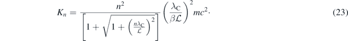
For the spherical well, the parameter β = 1 but β = 1/2 for the 1D well. As expected, the term between brackets in equation (23) is ∼2 when n = 1 and ≫ λ_C; thus, K₁ ≪ mc² and K₁ given by equation (23) coincides with the energies of the infinite wells calculated using the Schrödinger equation [4]. In contrast, when the dimension of the well is close to λ_C, the minimum particle energy is quasi-relativistic; therefore, equation (23) must be used. This implies a fundamental connection between quantum mechanics and especial theory of relativity. From equation (23) follows that K > 2mc² if a single particle with mass was confined in a volume much smaller than λ_C³. But when this happen the number of particles may not be constant anymore; therefore, a single point-particle with mass cannot exist. Only in fully relativistic quantum field theories, where the number of particles is not constant, point-particles with mass can exist [11–13]. This is a fundamental and general statement in relativistic quantum mechanics [7, 8]. Introducing the quasi-relativistic equation then provides a simple but precise way to present this concept in introductory quantum mechanics courses. Moreover, due to the fact that this statement just refers to the confinement of a particle with mass, one could adventure the following far reaching consequences: it is impossible to confine a single particle with mass in a point, this should be true for an electron, a quark, and probably may also be true for a black hole and the whole Universe at the beginning of the Big Bang.

Solving equation (1) for the Coulomb potential in hydrogen-like atoms allows for checking the validity of the quasi-relativistic wave equation. Moreover, this also permits to find out what is included and what is not in the quasi-relativistic approximation. Due to its importance, a summary of the solution of the quasi-relativistic wave equation for hydrogen-like atoms is given in the appendix . The values of Ę for the bound states calculated by solving equation (1) are approximately given by the following equation [13]:

$$\begin{equation}\it{\unicode{280}}_{n,l}\sim \it{\unicode{280}}_{n,\mathrm{S}\mathrm{c}\mathrm{h}}{Z}^{2}\left(1+\frac{2{\alpha }^{2}}{n\left(2l+1\right)}\right).\end{equation} \tag{ 24 }$$

In equation (24), Z is the atomic number, l is an integer in the interval from 0 to (n − 1), α is the fine-structure constant [7, 8]:

$$\begin{equation}\alpha =\frac{1}{4\pi {\varepsilon }_{o}}\frac{{e}^{2}}{\hslash c}\sim 1/137.\end{equation} \tag{ 25 }$$

And Ę_n,Sch corresponds to the bounded energies values of the electron in the hydrogen atom calculated using the Schrödinger equation [2–4]:

$$\begin{equation}\it{\unicode{280}}_{n,\mathrm{S}\mathrm{c}\mathrm{h}}=-\left[\frac{\mu }{2{\hslash }^{2}}{\left(\frac{{e}^{2}}{4\pi {\varepsilon }_{o}}\right)}^{2}\right]\frac{1}{{n}^{2}},\quad n=1,2,3,\dots .\end{equation} \tag{ 26 }$$

In equation (26), μ=(m_em_n)/(m_e + m_n) is the reduced mass of the electron in a hydrogen-like atom with a nucleus of mass m_n; m_e and e are the electron mass and charge, respectively; and ε_o is the electric permittivity of vacuum.

The exact values of Ę_n,l, which are calculated by exactly solving equation (1) as described in the appendix, can be validated by comparing them to the electron energies calculated by adding, as a first perturbative correction, the relativistic correction to equation (26), i.e. comparing to the values obtained using the following expression [4, 14]:

$$\begin{equation}\it{\unicode{280}}_{n,l,\mathrm{T}\mathrm{h}}\sim \it{\unicode{280}}_{n,\mathrm{S}\mathrm{c}\mathrm{h}}{Z}^{2}\left\{1-\frac{{\alpha }^{2}}{{n}^{2}}\left[\frac{3}{4}-\frac{n}{l+\frac{1}{2}}\right]\right\}.\end{equation} \tag{ 27 }$$

Table 1 shows energy differences values in meV corresponding to the hydrogen's (Z = 1) electron states with n = 1, 2 and 3. The values in the second column corresponds to the difference between the exact values of Ę_nl calculated by solving the equation (A16) as described in the appendix, and the values of Ę_n,Sch given by equation (26). The energy difference values in the third column corresponds to the difference between the values of Ę_nl,Th given by equation (27) and the values of Ę_n,Sch. By comparing the values reported in both columns, as should be expected because the relativistic correction includes the difference between the correct relativistic and the non-relativistic expression of K [4, 14], one can conclude that the electron energies calculated using the quasi-relativistic wave equation (equation (1)) includes the relativistic correction to the energy calculated in traditional first order perturbation theory [4, 14]. This also permits to realize the limitations of equation (1). It is well-known that the Dirac equation is the correct relativistic equation for describing the bounded states of the electron in a hydrogen-like atom [7, 8]. Besides the relativistic correction to K, two other corrections to equation (26) should be included for describing the fine structure of the hydrogen spectrum [14]. Neither the Darwin nor the spin–orbit corrections are included in the quasi-relativistic wave equation [13, 14]. Nevertheless, it is good to emphasize that equation (1) exactly includes the correct relativistic relation between p and K. The quasi-relativistic wave equation for hydrogen-like atoms can be exactly solved [13], while the relativistic correction included in equation (27) is just an approximate result.

The superposition principle is one of the pillars of quantum mechanics [1–4]. The Schrödinger, the Klein–Gordon, and the Dirac equations are all linear equations. However, neither the quasi-relativistic wave equation nor equation (10) are linear [11]. For instance, let be ψ₁and ψ₂ two solutions of equation (1) for the infinite well problem, and corresponding to different values of V²; then, ψ₁and ψ₂ would not be solutions of the same equation (1) but of slightly different equation (1) with different values of γ_V. Moreover, the wave function ψ = aψ₁ + bψ₂ would not be a solution of any equation (1). Consequently, if the quasi-relativistic wave equation could be a foundational equation, then the validity of the superposition principle in quantum mechanics should be questioned or revised [11]. May be this is why Schrödinger settled for the equation named after him instead of using a non-linear quasi-relativistic wave equation, which can be solved with no more difficulties than the ones present when solving the Schrödinger equation, but gives more precise results than the equation that he chose. Nevertheless, the existence of such non-linear equation rises the intriguing possibility of a quantum mechanics based on a non-linear wave equation. This is currently important because it is often assumed that the superposition state ψ represent a qubit, concept that is at the heart of current attempts for demonstrating a practical quantum computer [15, 16]. Would the eventual demonstration of a quantum computer exclude the possible existence of a quantum mechanics without a superposition principle? Could exist an alternative explanation of the eventual demonstration of a quantum computer that was based in a foundational non-linear wave equation? These are fascinating questions of current interest that are motivated by a third option that may be Schrödinger did not consider.

Alternatively, and this is the author's opinion and also the current prevalent opinion in the physicists' community, the non-linearity of the quasi-relativistic wave equation indicates that equation (1) is not a foundational wave equation but a kind of eigenvalue equation like, for instance, equations (17) and (A9) (shown in the appendix ). This can be made evident by using equation (7) for eliminating γ_V from equation (1), thus rewriting equation (1) as the following eigenvalue equation where ψ and Ę should be found simultaneously:

$$\begin{equation}i\hslash \frac{\partial }{\partial t}\psi =-\frac{{c}^{2}{\hslash }^{2}}{\left[\it{\unicode{280}}-U\right]+2\mu {c}^{2}}{\nabla }^{2}\psi +U\psi .\end{equation} \tag{ 28 }$$

While both forms of the same equation are equivalent, equation (1) is more suggestive due its striking similarity to the Schrödinger equation. The foundational equation corresponding to equations (1) and (28) is then the Klein–Gordon equation, which is linear and Lorentz invariant. For instance, let be ψ₁and ψ₂ two solutions of the non-linear 1D quasi-relativistic wave equation (equation (14)), for a particle in an infinite well, and corresponding to different values of Ę = K; therefore, the wavefunction ψ = aψ₁ + bψ₂ is not a solution of equation (14). However, due to equation (12), a solution of equations (8) and (10) can be found from a solution of equation (14) in the following way:

$$\begin{equation}{\psi }_{\mathrm{K}\mathrm{G}+}\left(x,t\right)=\psi \left(x,t\right){\mathrm{e}}^{-\mathrm{i}{\mathrm{w}}_{m}t},\quad {\mathrm{w}}_{m}=\frac{m{c}^{2}}{\hslash }.\end{equation} \tag{ 29 }$$

Therefore, if ψ_KG+,1 and ψ_KG+,2 are respectively related to ψ₁ and ψ₂ through equation (29); then, the wavefunction ψ_KG+,1,2 = aψ_KG+,1 + bψ_KG+,2 is not a solution of the non-linear equation (10) but, due to the linearity of equation (8), ψ_KG+,1,2 is a solution of the 1D Klein–Gordon equation. From this point of view, equation (1) provides a useful way to find exact solution of the Klein–Gordon equation with positives energies when Ę = K + U < 2mc². The Schrödinger equation then appears as a limit case of the quasi-relativistic wave equation when Ę ≪ 2mc². Luckily, the Schrödinger equation recovers the linearity required by the superposition principle. This allowed Schrödinger to construct a non-relativistic quantum mechanics based on the equation named after his genius.

Several properties of the solutions of the quasi-relativistic wave equation were summarized and discussed. It was shown that this quasi-relativistic equation can be solved following the same procedures and mathematical techniques needed for solving the Schrödinger equation; however, the results obtained are valid for particle energies where the correct relativistic relation between p and K must be used. This suggests the academic use of the quasi-relativistic wave equation for introducing the students to the implications of the special theory of relativity in introductory quantum mechanics courses. In addition, several consequences that would follow from using this quasi-relativistic wave equation as a quantum mechanics foundational equation were discussed. It was argued that no single particle with mass can be confined in a point, and it was suggested that this statement may be extrapolated to black holes and the whole Universe at the beginning of the Big Bang. It was also suggested that the current febrile competition for demonstrating a practical quantum computer obligates us to think about the possibility or not of the existence of a quantum mechanics theory based on a non-linear foundational wave equation. Finally, the existing relationship between the quasi-relativistic wave equation and the Klein–Gordon equation was clarified.

The quasi-relativistic wave equation for hydrogen-like atoms is given by the following expression [13]:

$$\begin{equation}i\hslash \frac{\partial }{\partial t}\psi \left(\rightharpoonup {r},t\right)=-\frac{{\hslash }^{2}}{\left[{\gamma }_{V}\left(r\right)+1\right]\mu }{\nabla }^{2}\psi \left(\rightharpoonup {r},t\right)+{U}_{\mathrm{C}}\left(r\right)\psi \left(\rightharpoonup {r},t\right).\end{equation} \tag{ A1 }$$

The Coulomb potential is given by

$$\begin{equation}{U}_{\mathrm{C}}\left(r\right)=-\frac{{e}^{2}}{4\pi {\varepsilon }_{o}}\frac{Z}{r}.\end{equation} \tag{ A2 }$$

Equation (A1) can be solved looking for a solution of the form [1, 13]:

$$\begin{equation}\psi \left(r,\theta ,\varphi ,t\right)=R\left(r\right)\Omega \left(\theta ,\varphi \right){\mathrm{e}}^{\frac{\mathrm{i}}{\hslash }Et}.\end{equation} \tag{ A3 }$$

Substitution of equation (A3) in equation (1) then results in [1, 13]:

$$\begin{equation}\frac{1}{r}\frac{{\mathrm{d}}^{2}}{\mathrm{d}{r}^{2}}\left(rR\right)+\frac{\left[{\gamma }_{V}\left(r\right)+1\right]\mu {r}^{2}}{{\hslash }^{2}}\left[E-U\left(r\right)\right]R=-l\left(l+1\right)\frac{R}{{r}^{2}}.\end{equation} \tag{ A4 }$$

And:

$$\begin{equation}{\Omega }_{l,m}\left(\theta ,\varphi \right)={Y}_{l}^{\left(m\right)}\left(\theta ,\varphi \right),\quad l=0,1,2\dots ;\enspace m=-l,-l+1,\dots 0,1,\dots ,l.\end{equation} \tag{ A5 }$$

In equation (A5), Y_l^(m) are the spherical harmonic functions [1–5]. equation (A4) can be solved making R(r) = χ(r)/r, then resulting the following equation [4, 13]:

$$\begin{equation}\frac{{\mathrm{d}}^{2}}{\mathrm{d}{r}^{2}}\chi \left(r\right)+\frac{\left[{\gamma }_{V}\left(r\right)+1\right]\mu }{{\hslash }^{2}}\left[\it{\unicode{280}}-{W}_{\mathrm{C}}\left(r\right)\right]\chi \left(r\right)=0.\end{equation} \tag{ A6 }$$

With:

$$\begin{equation}{W}_{\mathrm{C}}\left(r\right)=\left[{U}_{\mathrm{C}}\left(r\right)+\frac{{\hslash }^{2}}{\left[{\gamma }_{V}\left(r\right)+1\right]\mu }\frac{l\left(l+1\right)}{{r}^{2}}\right].\end{equation} \tag{ A7 }$$

As expected, when V ≪ c then γ_V ∼ 1; therefore, equation (A7) reduces to the radial equation of a hydrogen-like atom obtained using the Schrödinger equation [4]. Using equation (7), it is possible to eliminate γ_V from equations (A6) and (A7) by making

$$\begin{equation}\frac{\left[{\gamma }_{V}\left(r\right)+1\right]\mu }{{\hslash }^{2}}=\frac{K+2\mu {c}^{2}}{{c}^{2}{\hslash }^{2}}=\frac{\left[\it{\unicode{280}}-{U}_{\mathrm{C}}\left(r\right)\right]+2\mu {c}^{2}}{{c}^{2}{\hslash }^{2}}.\end{equation} \tag{ A8 }$$

Using equation (A8) then allows for rewriting equation (A6) in the following way [13]:

$$\begin{equation}\left\{-\frac{{\hslash }^{2}}{2\mu }\frac{{\mathrm{d}}^{2}}{\mathrm{d}{r}^{2}}\chi \left(r\right)-\left[\it{\unicode{280}}-{U}_{\mathrm{C}}\left(r\right)\right]\chi \left(r\right)+\frac{{\hslash }^{2}}{2\mu }\frac{l\left(l+1\right)}{{r}^{2}}\chi \left(r\right)\right\}-\frac{1}{2\mu {c}^{2}}{\left[\it{\unicode{280}}-{U}_{\mathrm{C}}\left(r\right)\right]}^{2}\chi \left(r\right)=0.\end{equation} \tag{ A9 }$$

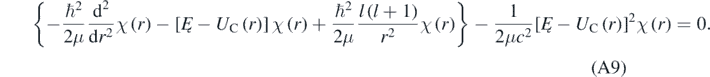
The term between braces in equation (A9) coincides with the radial equation that should be solved when using the Schrödinger equation [4]. The last term of equation (A9) can be disregarded when K ≪ μc²; therefore, the last term is a quasi-relativistic correction to the non-relativistic radial equation. Proceeding like it is done when solving the non-relativistic radial equation, one can introduce [4, 13]

$$\begin{equation}\zeta =\frac{1}{\hslash }\sqrt{-2\mu \it{\unicode{280}}}.\end{equation} \tag{ A10 }$$

For bound states, Ę < 0; therefore, ζ is real. Using equation (A10) allows for rewriting equation (A9) in the following way [4, 13]:

$$\begin{equation}\frac{{\mathrm{d}}^{2}}{\mathrm{d}{\rho }^{2}}\chi \left(\rho \right)=\left[{\rho }_{1}-\frac{{\rho }_{o}}{\rho }+\frac{l\left(l+1\right)-{\alpha }^{2}{Z}^{2}}{{\rho }^{2}}\right]\chi \left(\rho \right).\end{equation} \tag{ A11 }$$

With:

$$\begin{equation}\rho \equiv \zeta r,{\rho }_{o}\equiv \left(\frac{\mu {e}^{2}}{2\pi {\varepsilon }_{o}{\hslash }^{2}\zeta }-\alpha \frac{\hslash \zeta }{\mu c}\right)Z,\quad {\rho }_{1}\equiv \left[1-{\left(\frac{\hslash \zeta }{2\mu c}\right)}^{2}\right].\end{equation} \tag{ A12 }$$

Formally, when ℏζ ≪ μc and if α was null, then equations (A11) and (A10) would reduce to the corresponding equations obtained when solving the Schrödinger equation [4]; therefore, there is a relativistic correction in each term inside the brackets in equation (A11). Looking for a solution of equation (A11) of the following form [13]:

$$\begin{equation}\chi \left(\rho \right)\equiv \tau \left(\rho \right){\rho }^{\frac{1}{2}\left[1+\sqrt{{\left(1+2l\right)}^{2}-4{\alpha }^{2}{Z}^{2}}\right]}{\mathrm{e}}^{-\sqrt{{\rho }_{1}}\rho }.\end{equation} \tag{ A13 }$$

Results [13]:

$$\begin{align}\hfill & \rho \frac{{\mathrm{d}}^{2}}{\mathrm{d}{\rho }^{2}}\tau \left(\rho \right)+\left[1-\left(2\sqrt{{\rho }_{1}}\right)\rho +\sqrt{{\left(1+2l\right)}^{2}-4{\alpha }^{2}{Z}^{2}}\right]\frac{\mathrm{d}}{\mathrm{d}\rho }\tau \left(\rho \right)\hfill \\ \hfill & \quad +\left[{\rho }_{o}-\sqrt{{\rho }_{1}}\left(1+\sqrt{{\left(1+2l\right)}^{2}-4{\alpha }^{2}{Z}^{2}}\right)\right]\tau \left(\rho \right)=0.\hfill \end{align} \tag{ A14 }$$

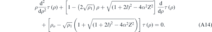
Again, as expected, if the quasi-relativistic corrections are very small, then equation (A14) reduces to the one obtained when using the Schrödinger equation [4, 13]. Finally, assuming that τ(ρ) can expressed as a finite power series in ρ [4, 13]:

$$\begin{equation}\tau \left(\rho \right)=\sum _{j=0}^{{j}_{\mathrm{max}}}{a}_{j}{\rho }^{j}.\end{equation} \tag{ A15 }$$

And substituting equation (A15) in equation (A14) results [13]:

$$\begin{equation}{\rho }_{o}=\left[2n+\mathbf{\Delta }\left(l,Z\right)\right]\sqrt{{\rho }_{1}}.\end{equation} \tag{ A16 }$$

With:

$$\begin{equation}\mathbf{\Delta }\left(l,Z\right)=\left[\left(1+\sqrt{{\left(1+2l\right)}^{2}-4{\alpha }^{2}{Z}^{2}}\right)-2\left(l+1\right)\right].\end{equation} \tag{ A17 }$$

Formally, when ℏζ ≪ μc and if α was null, then equation (A16) would reduce to ρ_o = 2n, with n = j + l + 1, which is the resulting equation when solving the Schrödinger equation [4]. It is worth noting that the author was able to find an exact analytical expression for Ȩ by substituting ρ_o and ρ₁ given by equation (A12) in equation (A16), solving the resulting equation for ζ, and then using equation (A10) [17]. The exact quasi-relativistic value Ȩ now depends not only on the principal quantum number n, but also on the angular quantum number l and Z. However, a simpler result easier to use can be found, for instance, assuming that the quasi-relativistic corrections included in ρ_o and ρ₁ do not need to be accounting for because they are too small. Consequently, the effect of the quasi-relativistic correction included in the centrifugal term in equation (A11) is quantified by the following equation [13]:

$$\begin{equation}\it{\unicode{280}}_{n,l}=-\left[\frac{\mu }{2{\hslash }^{2}}{\left(\frac{{e}^{2}}{2\pi {\varepsilon }_{o}}\right)}^{2}\right]\frac{{Z}^{2}}{{\left[2n+{\Delta}\left(l,Z\right)\right]}^{2}}.\end{equation} \tag{ A18 }$$

As expected, if α was null and Z = 1, equation (A18) would be identical to Ȩ_n,Sch given by equation (26). Equation (A18) can be rewritten as

$$\begin{equation}\it{\unicode{280}}_{n,l}=-\mu {c}^{2}{\alpha }^{2}{Z}^{2}\frac{1}{{\left[2n+{\Delta}\left(l,Z\right)\right]}^{2}}.\end{equation} \tag{ A19 }$$

Then equation (24) can be obtained from equation (A19) using the following approximated relations:

$$\begin{equation}\frac{1}{{\left[2n+{\Delta}\left(l,Z\right)\right]}^{2}}\sim \frac{1}{{\left(2n\right)}^{2}}\left[1-\frac{{\Delta}\left(l,Z\right)}{n}\right].\end{equation} \tag{ A20 }$$

And:

$$\begin{equation}\mathbf{\Delta }\left(l,Z\right)\sim -\frac{2{\alpha }^{2}}{2l+1}.\end{equation} \tag{ A21 }$$