


Abstract
Rutherford backscattering spectrometry is a nuclear analysis technique widely used for materials science investigation. Despite the strict technical requirements to perform the data acquisition, the interpretation of a spectrum is within the reach of general physics students. The main phenomena occurring during a collision between helium ions—with energy of a few MeV—and matter are: elastic nuclear collision, elastic scattering, and, in the case of non-surface collision, ion stopping. To interpret these phenomena, we use classical physics models: material point elastic collision, unscreened Coulomb scattering, and inelastic energy loss of ions with electrons, respectively. We present the educational proposal for Rutherford backscattering spectrometry, within the framework of the model of educational reconstruction, following a rationale that links basic physics concepts with quantities for spectra analysis. This contribution offers the opportunity to design didactic specific interventions suitable for undergraduate and secondary school students.
Export citation and abstract BibTeX RIS
1. Introduction
Modern physics has been introduced in the curricula of all European countries, starting from secondary school level. Besides teaching the new theories of quantum mechanics, as well as the issues on which they are based, a complementary contribution consists of giving students the opportunity to experience how researchers work in applied research labs and, in particular, how basic physics concepts ground the analysis techniques. It is important for students to learn that in physics the discovery and understanding of a phenomenon often lead to the development of new applications and analysis techniques, which open novel technological/research fields and allow measurements never possible before.
Rutherford backscattering spectrometry (RBS) (Chu et al 1978, Feldman and Mayer 1986), chronologically the first of the ion beam analysis (IBA) techniques developed in the early 20th century, is based on the famous Rutherford experiment (Rutherford 1911, 2012). An RBS measurement consists of sending a monoenergetic, collimated, light ion beam (typically H+ or He++) towards the surface of a sample, and in the collection of the energy spectrum of the ions of the beam which, after a collision with the target atoms, are backscattered along a certain direction into the active area of a solid-state detector. After RBS, other IBA techniques have been developed according to the various phenomena occurring in ion-matter interactions4 : Particle-induced x-ray emission (Chadwick 1913), where the x-ray emitted by the target atoms is analyzed, elastic non-Rutherford backscattering spectrometry (Chadwick and Bieler 1921), where the ion energy allows the target atom Coulomb barrier to be exceeded, and nuclear reaction analysis (Rutherford and Chadwick 1922), where nuclear reactions are caused between ions and target atoms. The great virtue of RBS among IBA techniques is its simplicity, which has enabled its establishment as a primary reference method for non-destructive materials science analyses (Jeynes 2017) in electronics, chemistry, earth science, works of art, and, in general, in applied sciences.
It is its very simplicity that makes RBS pedagogically attractive, because it is a modern physics technique with results that are interpreted by means of classical physics concepts, without the need of quantum mechanics knowledge. According with our experience (Michelini and Santi 2008, Corni 2008, 2010, Michelini 2010b, Mossenta 2010, 2012, Battaglia et al 2011), RBS can be integrated in university general physics courses as well as in the secondary school curriculum in its vertical development, allowing students to understand the role of conservation principles and of fundamental quantities, e.g. cross-section, in theory and in applications.
Although many physics education contributions concern the Rutherford experiment and the scattering cross-section, either theoretically (Chong and Andrews 1993, Gauthier 2000), or experimentally (Wicher 1965, Lee et al 1968, Eaton and Cheetham 1973, Grober et al 2010), RBS is completely ignored.
In this paper, within the theoretical framework of the model of educational reconstruction (Duit et al 2005) and by means of the Design-Based Research (DBR 2003, Lijnse 1995), intervention modules are carried out to develop and test research-based learning proposals (Anderson and Shattuck 2012) for vertical teaching-learning paths based on experimental work (Michelini 2010a, Michelini et al 2016).
We will present the educational proposal for RBS organized in terms of key questions to offer the teacher the opportunity to structure didactic specific interventions suitable for every context. We follow a rationale (table 1) linking basic physics concepts (table 1, first column) with quantities for spectra analysis (table 1, second column).
Table 1. Rationale of the RBS proposal.
| Basic physics concepts | Correlated quantities for spectra analysis |
|---|---|
| Ion-nucleus collision | Kinematic factor |
|
|
|
|
| Ion Coulomb scattering | Scattering cross-section |
|
|
|
|
|
|
| Ion inelastic stopping | Stopping cross-section |
|
|
|
|
2. What is RBS?
Although RBS measurements require large facilities to get the spectra (a MeV ion accelerator to produce the probe beam, vacuum lines to manage and transport the beam, a sample vacuum chamber where the collision between the beam and the sample occurs, and electronic data acquisition systems to detect and analyze the signals), RBS analysis is within the reach of everyone, because of the simplicity of the underlying concepts.
RBS spectra provide information about mass and depth distribution of the constituent elements in the first few hundred nanometers of a sample surface. Under certain conditions of beam and sample alignment, channeling-RBS (Feldman and Mayer 1982) spectra also provide information about the crystal order, kind of defects and damage profile in crystalline samples. With the geometrical setup (grazing incidence and detection angles) allowing the detection of recoiling target atoms in the forward direction, light-element profiling is performed with forward recoil spectrometry (Feldman and Mayer 1986). In this paper, we will focus specifically on conventional RBS.
An RBS spectrum of a compound layered sample can be roughly seen as the superposition of the spectra of the single composing elements, weighted by the composition fraction, and displaced in energy according to the distance from the surface.
Figure 1 shows a typical RBS spectrum. The vertical axis shows the RBS yield, i.e. the fraction of backscattered ions normalized to the detector solid angle and to the energy calibration factor5 . The bottom axis reports the channel number coming from the multichannel analyzer, the top axis the ion energy, resulting after the channel-energy calibration. The expected energy edges of oxygen, silicon and titanium at the surface are marked.
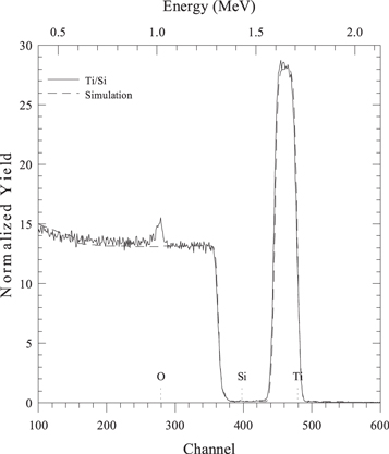
Figure 1. RBS spectrum (solid line) and simulation (dashed line) of a layer of 100 nm of Ti (peak at high energy) on a Si substrate (large band towards low energies), with a small contamination of oxygen (peak at about 1 MeV). Parameters of the measurement: beam energy 2.2 MeV, scattering angle 120°.
Download figure:
Standard image High-resolution image2.1. The features of RBS
From a didactic point of view, it is important that the students discuss the feature of RBS allowing the use of classical physics models, i.e. material point elastic collision, unscreened Coulomb scattering, and inelastic energy loss of ions with electrons.
2.1.1. Elastic collision
High-energy beam allows the interaction of the backscattered ion with matter to be considered as an elastic collision with an unscreened target atom nucleus. This condition avoids electron interaction that would cause energy loss.
The students easily evaluate the needed beam energy by imposing that the closest distance r reachable by a He ion of energy E in a head-on collision with an unscreened nucleus of a generic element of atomic number Z is smaller than the Bohr radius rB of a single electron ion of the element:

where a0 is the Bohr radius of hydrogen. The minimum energy results in 54Z2 in eV units, i.e. about 10 keV for Si, 330 keV for Au, and, however less than 1 MeV even for the heaviest target elements. Conventional RBS employs He ion beams of about 2 MeV.
2.1.2. Light ions
The use of light ions such as H+ or He++, or any with masses lower than those of the target atoms, makes the backscattering possible. In contrast, the ion would be scattered in the forward direction and lost into the material. Students verify this condition by studying the equations resulting from an activity in section 3.1.
2.1.3. Single scattering
In the case of non-surface scattering, ions lose energy in their inward and outward paths. Energy loss can be due to interactions with electrons and with nuclei.
Multiple scattering, in addition to that with the target nucleus, happens in particular for heavy elements and results in a lower energy of the emerging ion than that expected for a single scattering. By neglecting the low-energy part of an RBS spectrum, multiple scattering events and superimposition of signals are excluded.
Energy loss is then only due to electrons. For the very large number and very light mass of electrons, the loss is the result of numerous small losses that can be treated statistically and be thought of as a sort of uniform friction.
3. Inquiry-based approach to RBS
According to our experimental approach, the educational treatment of RBS follows a sequence of inquiry-type questions, to prepare a problem-solving activity. We are interested in obtaining information about the sample composition and structure from the spectra. First, we will focus on the particular case of surface elements (sections 3.1–3.2), then we will consider the more general case of elements buried in the first few hundred nanometers from the surface (section 3.3). For every topic, we supply experimented didactic activities (Michelini and Santi 2008, Corni 2008, 2010, Michelini 2010b, Mossenta 2010, 2012, Battaglia et al 2011) suitable for all kinds of student inclination and laboratory equipment: from theoretic calculation to experimental investigation, from computer simulation to application for materials analysis. We divide them into introductory activities (sections 3.1–3.3)—some of them inspired by the literature—about the single phenomenon of RBS, and advanced activities (section 3.4) about the RBS technique itself. Some introductory activities will concern macroscopic simulators of the atomic phenomena occurring in RBS, so the dependence of the various quantities on atomic number will disappear.
3.1. Atomic masses of the target atoms and the elastic nuclear collision
We are interested in identifying the elements present on the sample surface, i.e. in evaluating their atomic masses. The energy fractions of two material points after an elastic collision depends only on their masses, for a given scattering angle. By imposing the conservation of energy and momentum, and defining the kinematic factor  as the ratio between the ion energy after,
  and before, E0, the collision, we calculate the energy of an ion backscattered at angle θ as a function of the mass M of the target element.
Note that the calculation of the kinematic factor does not depend on the kind of interaction, i.e. the (conservative) force responsible for the scattering.
3.1.1. Didactic activity: calculation of the kinematic factor (introductory—student exercise)
By solving the conservation equations of (bi-dimensional) momentum and of kinetic energy of an impinging ion of mass m and energy  with a target atom of mass M initially at rest
where ϕ is the recoil scattering angle, we calculate the kinematic factor:

By studying this equation, we notice that the scattering angle allows the best mass resolution, i.e. the geometrical condition that produces the maximum change in  with a given (small) variation of M, is
  i.e. just the backscattering condition.
3.1.2. Didactic activity: measurement of the kinematic factor (introductory—experimental)
The kinematic factor, in the case of head-on collision  can be experimentally evaluated in the didactic laboratory using a macroscopic simulator with track and carts. A cart of known mass m, representing the ion, is sent towards a second cart with mass M > m initially at rest, representing the target atom, the two carts being equipped with spring bumpers. By means of sonar sensor measurements, the velocity of the first cart just before and after the collision is measured from the slope of position versus time graph. By varying M, the experimental kinematic factor as a function of m/M is obtained. Figure 2 shows the data compared to the theoretical expectation given by equation (3).
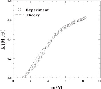
Figure 2. Experimental values of the kinematic factor using track and carts (m = 0.605 kg, 0.605 kg ≤ M ≤ 5.008 kg) compared to the theoretical expectation (equation (3)).
Download figure:
Standard image High-resolution image3.2. Fraction of an element and the unscreened Coulomb scattering
Once we have identified, by their energy, the backscattered ions coming from the atoms of a given element, we are interested in quantifying the surface fraction of this element. It is a statistical problem and for this, different from many textbooks that reduce the treatment to only geometrical considerations, it is important from an educational point of view (Corni et al 1996). We think in terms of RBS normalized yield  i.e. number of detected ions
  backscattered by the element atoms within a solid angle Ω around θ with respect to the total number of sent ions Ntot6
: this fraction is related to the number of atoms of the element per unit area and is strongly dependent on their atomic number. We have to calculate the probability
backscattered by the element atoms within a solid angle Ω around θ with respect to the total number of sent ions Ntot6
: this fraction is related to the number of atoms of the element per unit area and is strongly dependent on their atomic number. We have to calculate the probability  of scattering: in this case, we need to know the form of the ion-nucleus interaction, which determines the spreading of ion trajectories.
If we define the scattering cross-section  of an element of atomic number Z as this probability
  per unit solid angle for one atom of the element per unit area:

where n is the number of atoms per unit area, we calculate it theoretically by knowing the way ion trajectories are bent by the unscreened nucleus Coulomb force. The scattering cross-section is strongly dependent on the atomic number of the element, besides the scattering angle. Approximating probability with frequency, we then can evaluate the element surface density n through the experimental RBS normalized yield:

3.2.1. Didactic activity: calculation of the Rutherford scattering cross-section (introductory—student exercise)
The theoretical calculation of the scattering cross-section  of an element of atomic number Z requires the expression of
  We profit from the cylindrical symmetry and introduce the impact parameter
  as the distance between the ion original direction and the target nucleus (figure 3). If we consider one target atom in a unit surface, the ions collected in a solid angle
  are those coming from a ring area of radius
  and thickness db, i.e.
  where the relation between θ and
  is defined by the form of the interaction force. If S is the beam section area, D is the beam current section density, and t the measurement time interval,
  is the charge that will be collected after the scattering and SDt the total charge sent. Then:

where we have set n = 1 and S = 1. The minus sign means that  decreases with increasing θ.
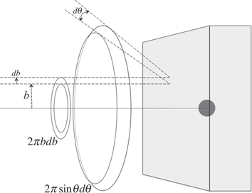
Figure 3. Geometrical illustration of the quantities used to calculate the scattering cross-section in equation (6).
Download figure:
Standard image High-resolution imageEquation (6) shows that the calculation of the scattering cross-section is a matter of finding the relation between the scattering angle and the impact parameter and of computing the derivative of  with respect to θ. By assuming the target atom at rest (i.e. no energy exchange during the collision), this calculation for He++ ions proves to be particularly simple, though introducing a small error7
with respect to the more general case of the recoiling target atom:
with respect to θ. By assuming the target atom at rest (i.e. no energy exchange during the collision), this calculation for He++ ions proves to be particularly simple, though introducing a small error7
with respect to the more general case of the recoiling target atom:

and

which is the well-known formula of the Rutherford backscattering cross-section. Hints for the calculation of equation (7) are in (Chu et al 1978).
3.2.2. Didactic activity: calculation of the hard-sphere scattering cross-section of a circular-shaped planar target (introductory—student exercise)
To give concreteness to this concept, students can be involved in the calculation of the scattering cross-section in the case of 2D elastic hard-sphere collision with forms of geometrical shapes. Equation (6), in a plane, reduces to  In the case of a circular form, from figure 4 (top), we find
  and
and


Figure 4. (top) Geometry leading to equation (9). (bottom) Geometrical construction of the shape of a planar target leading to the 2D Rutherford cross-section in the case of hard-sphere scattering.
Download figure:
Standard image High-resolution image3.2.3. Didactic activity: calculation of the shape of a planar form leading to the 2D Rutherford cross-section in the case of hard-sphere scattering (introductory—student exercise)
Recalling equation (7) and with reference to figure 4 (bottom), the slope of the tangent to the shape in the collision point is  leading to the equation for the form shape:

which is a parabola with y = 0 symmetry axis.
3.2.4. Didactic activity: measurement of the hard-sphere scattering cross-section of a circular-shaped planar form (introductory—experimental)
This activity, employing a macroscopic simulator, allows the students, perhaps for the first time, to be involved in and to reflect on the statistical character of the cross-section and about the quantities to be introduced into the equations, such as  and n.
The measurement of the scattering cross-section in the case of 2D hard-sphere collision can be performed using a glass marble and a wooden circular form. The marble is repeatedly launched along parallel, equally spaced, directions towards the form using a launch guide (figure 5(a)). The trajectories of the marble before and after the collision are traced (figure 5(b)), then the scattering angles are measured and tabulated according to a certain acceptance angle Δθ.
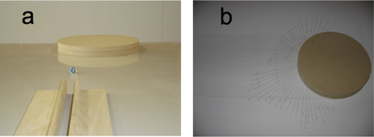
Figure 5. (a) Launch guide and circular wooden form for marble collision. (b) Tracking of the marble trajectories.
Download figure:
Standard image High-resolution imageFigure 6 reports the experimental scattering cross-section of a circular form of radius RF = 11,2 cm using a marble of radius rM = 2.2 cm with 88 equally spaced (0.5 cm) launches. In equations (4) and (9), we have substituted 
 and
and 
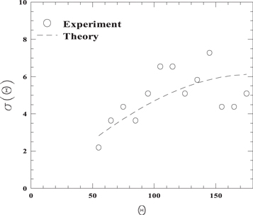
Figure 6. Measurements of the scattering cross-section of a circular form and expected theoretical curve.
Download figure:
Standard image High-resolution imageWith a similar procedure, the experimental cross-section of forms with different shapes, parabolic (see activity in 3.2.3 for its importance), elliptical, triangular, etc, can be measured.
3.3. Depth distribution of an element and inelastic ion energy loss
If the collision does not occur at the sample surface, the ion loses part of its energy, before hitting a nucleus. Moreover, this ion, in its back path, traverses again the layer before emerging from the sample surface. The detected ion energy results are lower than in the case of surface scattering due to the many small interactions with the electrons of matter: the deeper the target atom, the lower the ion energy. Due to the difficulties in modeling this statistical phenomenon, the differential energy loss of ions  strongly dependent on the atomic number besides the scattering angle, is evaluated experimentally for every element, where Z is the element mass, and E the ion energy. The quantity useful for RBS is the stopping cross-section, defined as the energy loss normalized by the element atomic density

The stopping cross-section is not affected by the different densities of the elements, and clearly exhibits a strong increase with atomic number, with small oscillations mostly due to the difference in orbital electronic density distribution (Chu et al 1978).
If we consider thin surface layers, we can approximate8
the stopping cross-section as constant like a friction parameter: at the sample surface value  in the inward path, and at the value after a scattering at the surface
  in the outward path. In this way, the energy loss in traversing a thickness
  is given by
  In an RBS spectrum, a homogeneous layer of thickness
  results in a nearly box-like energy band. The lower boundary is the energy
  of an ion emerging from the sample after a collision at a depth
  and having lost an amount of energy
  in its inward path and
  in the outward path. The higher boundary is the energy
  of an ion after a surface collision. The energy bandwidth of the RBS spectrum of a layer of thickness
  turns out to be
which, under the applied approximation, proves to be proportional to  Note that from an RBS spectrum, as from all the other nuclear techniques, we cannot obtain direct information about the thickness Δx of a layer, but only about the product
  i.e. the number of atoms of the element per unit area
  in the layer. This means that thicknesses are measurable once the atomic densities are known, or vice versa.
3.3.1. Didactic activity: Measurement of energy loss (introductory—experimental)
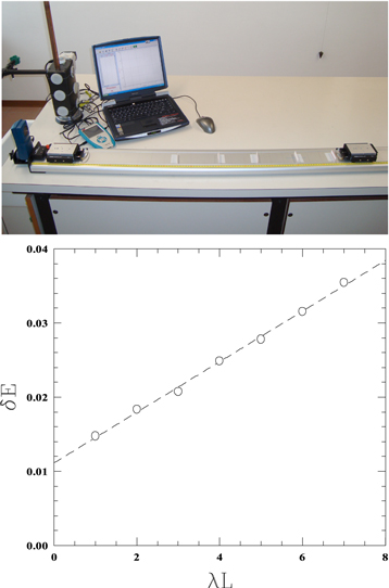
With the same macroscopic simulator of section 3.1.2, the role of the stopping of the impinging ion due to the crossing of matter can be evidenced. Small pieces of paper, e.g. post-its, are stuck, equally spaced, along the track. The post-it number per unit length λ represents the sample atomic density  in 1D, while the length L of the track segment with the post-its represents the thickness Δx of the layer.
  i.e. the number of post-its on the track, represents, in 1D, the number of atoms of the element per unit area in the layer
  After positioning a target cart of mass M = 2.108 kg on one side of the post-it layer, and measuring, with a sonar sensor, the velocity of the projectile cart of mass m = 0.605 kg entering and, after the collision, leaving the post-it segment, it is possible to evaluate the energy bandwidth
  in analogy to equation (12), under various conditions. Figure 7 (top) shows the measurement apparatus. Figure 7 (bottom) reports the measurement of
  as a function λL (from 1–7) with constant L (60 cm). The slope of the experimental points represents the term in parenthesis of equation (12). The non-zero intercept is an artifact of the experimental setup, due to the friction with the track.
Figure 7. (top) Experimental setup for measurements of energy loss with track and carts. (bottom) Energy bandwidth as a function of  (
( ) with constant L (
 ).
).
Download figure:
Standard image High-resolution image
The change of energy bandwidth with constant L, i.e. Δx, but with varying  i.e.
i.e.  allows us to recognize that, according to equation (12), with collision experiments, we cannot distinguish between thickness and atomic density of a layer.
3.4. RBS analysis
In summary, an RBS spectrum of a surface layer, with thickness  and atomic density
  of an element with atomic number ZS and mass MS results in a band, with the high-energy edge at
  width
width  (equation (12)) and normalized yield
  (equation (5)) (see the contribution of Ti in figure 1). In the case of a buried layer of an element of atomic number ZB and mass MB, the high-energy edge is displaced at lower values than
  (see the Si contribution in figure 1). The energy displacement can be calculated using equation (12) with suitable substitutions
  If a layer contains mixed elements or compounds, the yield of the RBS spectrum of every element of the layer will be scaled proportionally to the element fraction (equation (5)).
3.4.1. Didactic activity: qualitative simulation of RBS spectra (advanced—simulation)
Students are involved in drawing qualitative simulations of RBS spectra of given sample structures. Table 2 lists some examples of problems posed to the students and successfully solved. The masses (and the atomic numbers) of the elements A, B, C, and S are in the following order: 
Table 2. Sketches of simulated RBS spectra of some sample structures. The energy positions of the single elements at the surface are marked.
| Sample structure | Simulated qualitative RBS spectrum |
|---|---|
| Thin layer of element A on a substrate of element S |
|
| Thick layer of element A on a thin layer of element B on a substrate of element S |
|
| Layer of element C on a substrate of element S |
|
| Thin layer of element B on a thin layer of element A on a substrate of element S |
|
| Thick layer of element B on a thin layer of element A on a substrate of element S |
|
| Thin layer of compound AB on a substrate of element S |
|
| Thin layer of compound AB3 on a substrate of element S |
|
| Thin layer of compound AS on a substrate of element S |
|
3.4.2. Didactic activity: quantitative simulation of RBS spectra (advanced—simulation)
RUMP9 is a free package providing comprehensive analysis and simulation of RBS. Students generate RBS spectra, starting from a sample structure and composition, and see/discuss what happens by changing the element or sample structure, as well as measurement parameters (scattering angle, beam energy, etc). Initially, they reproduce some of the exercises proposed in table 2, using, for example, A = Zn, B = Ti, C = O, S = Si, then they imagine different and new sample structures (see table 3 for some key examples with RUMP commands to obtain the simulated spectra).
Table 3. Examples of sample structures, corresponding RUMP commands, and RBS simulated spectra. The expected energy positions of the single elements at the surface are marked.
| Sample structure | |
|---|---|
| 150 nm layer of element A on 150 nm layer of element B on a substrate of element S |

|
| Beam energy 2 MeV, scattering angle 160° | |
| RUMP commands: | |
| reset | |
| mev 2 | |
| theta 0 | |
| phi 20 | |
| sim layer 1 thickness 1500 A composition Zn 1/ | |
| next thickness 1500 A composition Ti 1/ | |
| next thickness 20 000 A composition Si 1/ | |
| FWHM 10 | |
| econv 3.3 100 | |
| lt 1 | |
| plot 0 | |
| element Zn element Ti element Si | |
| 500 nm layer of compound SC2 on a substrate of element S |
|
| Beam energy 2 MeV, scattering angle 160° | |
| RUMP commands: | |
| reset | |
| mev 2 | |
| theta 0 | |
| phi 20 | |
| sim layer 1 thickness 5000 A composition O 2 Si 1/ | |
| next thickness 20 000 A composition Si 1/ | |
| FWHM 10 | |
| econv 3.3 100 | |
| lt 1 | |
| plot 0 | |
| element O element Si | |
| 300 nm layer of compound AS on a substrate of element S. |
|
| Beam energy 2 MeV, scattering angle 160° | |
| RUMP commands: | |
| reset | |
| mev 2 | |
| theta 0 | |
| phi 20 | |
| sim layer 1 thickness 3000 A composition Zn 1 Si 1/ | |
| next thickness 20 000 A composition Si 1/ | |
| FWHM 10 | |
| econv 3.3 100 | |
| lt 1 | |
| plot 0 | |
| element Zn element Si | |
| 300 nm layer of element B on 80 nm layer of element A on a substrate of element S |
|
| Beam energy 2 MeV, scattering angle 160° | |
| RUMP commands: | |
| reset | |
| mev 2 | |
| theta 0 | |
| phi 20 | |
| sim layer 1 thickness 3000 A composition Ti 1/ | |
| next thickness 800 A co Zn 1/ | |
| next thickness 20 000 A co Si 1/ | |
| FWHM 10 | |
| econv 3.3 100 | |
| lt 1 | |
| plot 0 | |
| element Zn element Ti element Si | |
| 150 nm layer of element A on 150 nm layer of element B on a substrate of element S |
|
| Beam energy 2 MeV, scattering angle 120° | |
| RUMP commands: | |
| reset | |
| mev 2 | |
| theta 0 | |
| phi 60 | |
| sim layer 1 thickness 1500 A composition Zn 1/ | |
| ne thickness 1500 A composition Ti 1/ | |
| next thickness 20 000 A composition Si 1/ | |
| FWHM 10 | |
| econv 3.3 100 | |
| lt 1 | |
| plot 0 | |
| element Zn element Ti element Si | |
| 150 nm layer of element A on 150 nm layer of element B on a substrate of element S |
|
| Beam energy 2.5 MeV, scattering angle 160° | |
| RUMP commands: | |
| reset | |
| mev 2.5 | |
| theta 0 | |
| phi 20 | |
| sim layer 1 thickness 1500 A composition Zn 1/ | |
| next thickness 1500 A composition Ti 1/ | |
| next thickness 20 000 A composition Si 1/ | |
| FWHM 10 | |
| econv 3.3 100 | |
| lt 1 | |
| plot 0 | |
| element Zn element Ti element Si | |
RUMP, like many other of this kind, besides the spectra simulations, gives numerical values of kinematic factors, scattering and stopping cross-sections of every element and of some compounds. These values can be retrieved by students and used, for example, to study the behavior of these quantities as a function of the scattering angle and of the atomic number or mass10 .
3.4.3. Didactic activity: qualitative analysis of RBS spectra (advanced, analysis)
RBS spectra, no matter whether real or simulated, can be given to the students so that they can guess and discuss the structure and composition of the sample on the basis of their knowledge (see section 2). Some real RBS spectra are supplied with this paper (together with the simulation macros for RUMP), and others can be found on the Internet or in journal articles. In the absence of real data, the teacher can generate incognito RBS spectra through RUMP or use those of table 3.
3.4.4. Didactic activity: quantitative analysis of RBS spectra (advanced, analysis)
Using the same spectra, students, equipped with simulation software such as RUMP, experience the thrill of performing actual sample analyses.
Table 4. Blended training course for secondary school teachers.
| Duration | Mode | Description | Reference |
|---|---|---|---|
| 1 week | group | Reading about the basic concepts of RBS and discussion in forum both from a disciplinary and didactical point of view | sections 2 and 3 |
| 1 week | group | Analysis and discussion of RBS spectra | section 3.4.3 with spectra of table 2 |
| 1 week | individual | Design of a didactic path with the goal of allowing secondary school students to understand the basis of RBS and to interpret elementary spectra | |
| 8 h | plenary | Conduction of laboratory activities with 50 secondary school students | See table 5 |
The steps for a spectrum analysis we set up according to research-based intervention modules we experimented is organized in the following steps.
- Determine the element(s) of the surface layer. Proceeding from higher to lower energies, guess a possible element at the sample surface. If the element peak does not show the expected yield, it is possible that a compound surface layer is present. In this case, search for the other component(s) and determine the atomic composition of the surface layer.
- Calculate the thickness of the surface layer. Determine the thickness of the surface layer that accounts for the width(s) and the height(s) of the surface layer peak(s).
- With analogous procedure, determine elements, atomic compositions and thicknesses of the underlying layers.
- Determine the substrate composition.
Table 5. Segment of a general physics course for undergraduate students.
| Duration | Mode | Description | Reference |
|---|---|---|---|
| 1.5 h | seminar | Introduction to RBS: hypotheses, main phenomena and information we can get | section 2 |
| 1.5 h | group | Experimental and theoretical activities in parallel | sections 3.1–3.3 |
| 1 h | plenary | Discussion | |
| 30 min | seminar | Introduction to the interpretation of an RBS spectrum | section 3.4.4 |
| 1 h | group | Quantitative analysis of RBS spectra with simulation software | |
| 1 h | plenary | Discussion |
4. Research-based path proposal
The activities presented here are the follow-up of the research-based intervention modules we experimented in IDIFO summer schools for teachers in 2014 and for talented secondary school students from 2007–2016 (Michelini and Santi 2008, Corni 2008, 2010, Michelini 2010b, Mossenta 2010, 2012, Battaglia et al 2011). In tables 4, 5, and 6, we outline possible didactic sequences suitable for a training course for secondary school teachers, a general physics course for undergraduate students, and a laboratory for secondary school students, respectively.
Table 6. Modern physics laboratory for secondary school students.
| Duration | Mode | Description | Reference |
|---|---|---|---|
| 1 h | seminar | Introduction to RBS guided by concrete questions, oriented to obtain information from the spectra | sections 3.1–3.3 |
| 1 h | group | Experimental and theoretical activities in parallel | sections 3.1.1, 3.1.2, 3.2.4 |
| 40 min | plenary | Discussion of the results | |
| 20 min | seminar | Introduction to the interpretation of an RBS spectrum | See points in 3.4.4 |
| 1 h | individual | Interpretation of RBS spectra | Spectra of table 3 |
| 2 h | plenary | Discussion of the spectra interpretations | |
| 1 h | individual | Building of RBS spectra | Spectra of table 2 |
| 1 h | plenary | Discussion |
5. Summary
We have presented a variety of activities about RBS suitable for all kinds of student inclination and laboratory equipment. Some of them are introductory activities about the single phenomena of RBS, while others are advanced activities about the RBS technique itself. We have also exemplified how these activities can be composed into didactic paths, suitable for secondary school teachers, undergraduate and secondary school students.
The didactic proposal offers the opportunity for students to see how the historical Rutherford experiment leads to the development of a modern analysis technique such as RBS, based on classical physics and relying on the fundamental principles of conservation. Elastic nuclear collision, Coulomb scattering, and ion stopping are introduced through inquiry-type questions aimed at obtaining information about the composition and structure of a sample. Elastic nuclear collision leads to the definition of the kinematic factor. Mathematical calculation of the kinematic fraction makes the students study its behavior analytically, while track and carts allow them to measure the kinematic factor as a function of the target mass. The Coulomb scattering leads to the notion of scattering cross-section. The mathematical evaluation of the Rutherford scattering cross-section is an opportunity for students to discuss its analytical form together with the adoptable approximations. 2D reduction allows them to better visualize the cross-section analytical shape and to perform statistical measurements. Finally, ion stopping leads to the notion of stopping cross-section. Experiments with track and carts make the students reflect on the meaning of the energy bandwidth of the RBS spectrum of an element layer.
The activities about RBS challenge the students to engage their knowledge about the various phenomena to interpret or build RBS spectra. The availability of simulators, e.g. RUMP, allows the students to build and discuss spectra, starting from hypothetical sample structures and changing the parameters. Qualitative and quantitative didactic simulation activities are suggested. The students can also experience the thrill of performing real sample analyses. We propose activities of qualitative analysis where students interpret the RBS spectra by deduction from the equations, as well as activities of quantitative analysis following a fitting procedure with simulated data. Experimental RBS spectra are supplied with this paper, together with the RUMP macros giving the optimized simulations.
The experimentations, which have been performed during the last ten years in Italy, show quick and good responses from the students and teachers.
Acknowledgments
We thank Professor Giampiero Ottaviani of the University of Modena and Reggio Emilia, for introducing and training us to get and to analyze RBS spectra, Dr Rita Tonini for the valuable technical support, and Alessandra Mossenta for her valuable didactic work.
Footnotes
- 4
For a historical and complete review of IBA techniques, see (Chris Jeynes and Colaux 2016).
- 5
Ion energy calibration (the linear relation between the channel number and the ion energy—the calibration factor being the slope of this straight line) results from the analysis of RBS spectra of reference samples with known structure and composition.
- 6
The energy calibration factor, introduced in section 2, comes from numerical computation, here ignored for theoretical treatment.
- 7
The error increases with decreasing mass, e.g. 0.08% for Au and 6% for Na.
- 8
This approximation is called surface approximation.
- 9
RUMP (Computer Graphic Service) download page: http://genplot.com, command reference: http://genplot.com/doc/rump.htm.
- 10
Example of meaningful 3D graphs are reported in (Chu et al 1978).
Supplementary data (146 B MAC) Simulation macro 1.
Supplementary data (1.6 KB RBS) Real RBS spectra 1.
Supplementary data (146 B MAC) Simulation macro 2.
Supplementary data (1.6 B RBS) Real RBS spectra 2.
Supplementary data (175 B MAC) Simulation macro 3.
Supplementary data (1.6 KB RBS) Real RBS spectra 3.
Supplementary data (139 B MAC) Simulation macro 4.
Supplementary data (1.7 KB RBS) Real RBS spectra 4.
Supplementary data (189 B MAC) Simulation macro 5.
Supplementary data (1.7 KB RBS) Real RBS spectra 5.
Supplementary data (118 B MAC) Simulation macro 6.
Supplementary data (1.6 KB RBS) Real RBS spectra 6.
Supplementary data (147 B MAC) Simulation macro 7.
Supplementary data (1.6 KB RBS) Real RBS spectra 7.