
Abstract
Virtual shunt describes the overall loss of O2 content between the alveolar gas and arterial blood. Clinicians indirectly estimate the magnitude of the virtual shunt by monitoring peripheral blood oxygen saturation (SpO2) using non-invasive pulse oximetry. An inherent limitation of this method is the variable precision of pulse oximeters and the non-linear relationship between virtual shunt and SpO2 which is rarely depicted.
We propose a model using a combination of basic physiological equations to analyze the estimation of virtual shunt from inspired oxygen (FiO2) and SpO2. The model emphasizes the effect of the non-linearity of the Hb–O2 dissociation curve. Furthermore, it accounts for the variability in SpO2 measurements due to the precision of pulse oximeters.
The model was validated with experiments conducted on healthy subjects in a normobaric hypoxia chamber comparing the simultaneous readings from two different commercial pulse oximeters at FiO2 = 21% and 17%. SpO2 probability distributions calculated from the model were estimated. Although a variable bias (1.2–2.1%) in SpO2 between the pulse oximeter brands was observed, the tested pulse oximeters were both within tolerance specified by the manufacturers and matched the probability distributions from the model.
The theoretical and experimental findings show that the estimation of virtual shunt is challenging with a single SpO2 measurement using pulse oximeters with tolerances of 2%. Clinical decisions must be based on an appreciation of these limitations.
Export citation and abstract BibTeX RIS
1. Introduction
Pulse oximeters have become essential noninvasive monitoring devices in operating rooms and intensive care units for measuring the peripheral oxygen saturation (SpO2) and heart rate. The clinician is reassured by an SpO2 of 98–100% when the patient is breathing room air at sea level. Concerns arise when the SpO2 is less than 96% or drops from 99% to 96% or more in a healthy patient. The technical limitations and environmental effects (such as altitude) of the measurement of SpO2 must be appreciated by the clinician to ensure appropriate clinical decision making. For example, SpO2 of 99% or 100% are not physiologically plausible in a healthy subject breathing room air oxygen concentrations. This is due to the oxygen affinity of hemoglobin and the resulting hemoglobin–oxygen (Hb–O2) dissociation curve (West 2012). This frequent overestimation of high SpO2 is attributed to measurement tolerances of pulse oximeters and is device and brand specific (Webb et al 1991).
An inherent limitation of pulse oximeters is the relatively large tolerance intervals (±2–3%) leading to a low precision of the arterial blood oxygen saturation (SaO2) estimation. Technical limitations of pulse oximeters and subject variability contribute to these large measurement inaccuracies. The agreement of measurements is affected by light-tissue interactions, sensor manufacturing variations, manufacturer specific in vivo calibrations, and variations in application and handling of the probe. All of these factors can introduce errors in the SaO2 estimation, potentially leading to inadequate intervention (Jubran 1999). Knowledge of the accuracy of the performed estimation is essential for appropriate clinical decision making (Weininger 2007). To assess the reliability of the provided measure, clinicians must be aware of the device limitations.
Device specification standards demand reporting the expected accuracy of the SpO2 reading in the device manual (ISO 2011). However, in clinical diagnostic situations, a binary decision is frequently required (normal or abnormal SpO2). For example, when determining the presence of hypoxemia in a critically ill patient, a fixed classification threshold of 90% is typically used, but with the observed inaccuracy in the estimation, thresholds of up to 94% have been suggested (Van de Louw et al 2001). In such situations an inaccurate knowledge of the SaO2 can severely under- or overestimate the severity of the underlying disease process and lead to inaccurate treatments (Van de Louw et al 2001).
Virtual shunt (VS) is a theoretical concept that describes the overall loss of O2 content between the alveolar gas and arterial blood (West 2012). Estimating VS is of importance to the clinician as the magnitude of shunt describes the efficiency of the gas exchange and severity of a disease process causing a reduction in oxygenation. Shunt is measured in the clinical setting using a pulmonary artery catheter. However, in practice this is rarely available. Instead, VS is typically estimated from oxygen partial pressure measurements of the arterial blood (PaO2), obtained from blood gas analysis. Since SpO2 obtained from pulse oximetry is an estimate of the SaO2, the magnitude of VS could be indirectly estimated using this non-invasive device. However, in clinical applications where individual measurements are performed and a single SpO2 measure is taken, the wide distribution of possible SaO2 values should be appreciated when estimating VS.
Portable pulse oximeters are increasingly used as spot-check devices where sampling of arterial blood is not available. The availability of very few data points poses an increased challenge in the estimation of VS. In this study we describe a model to estimate VS from pulse oximeter readings. The model illustrates the impact of accuracy of pulse oximeters. We provide a mathematical, physiological framework to describe the propagation of specified tolerances of pulse oximeter readings in the estimation of oxygen saturation across the different stages of the oxygen cascade used for the estimation of the VS. The estimation of the SaO2 value based on measured SpO2 readings and the oxygen cascade has application in automated decision making algorithms. Providing the level of certainty (tolerance intervals) with each measurement may help increase awareness among medical personnel of limitations in pulse oximeter accuracy.
1.1. Background
The fundamental principle of pulse oximetry is a light-tissue interaction. The absorption of light by tissue depends on the wavelength, the tissue composition and the distance (optical path) traveled by the light which changes with each heart beat as blood volume in vessels changes. SaO2 describes the percentage of oxygenated hemoglobin over the total functional hemoglobin and can be estimated through measuring the ratio (R) of pulsatile and nonpulsatile components of the nonabsorbed light at two distinct wavelengths (typically 660 nm and 910 nm). The relationship between R and SaO2 can be theoretically explained with the Beer–Lambert law. However this description ignores scattering of light (Mannheimer 2007) and various other design aspects of oximeters, such as optical shunt or probe type. To account for these effects, the relationship between R and SpO2 is empirically determined by pulse oximeter manufacturers for each device. Even with empirical calibration, SpO2 remains only an estimate of SaO2.
The design of pulse oximeters is currently regulated by the International Standards Organization (ISO) specification ISO 80601-2-61 (ISO 2011). This standard describes the requirements for the design of pulse oximeters such as packaging, electro-magnetic safety, alarms, and display. Further, the standards give recommendations on the performance of calibration experiments using desaturation studies with human subjects, including testing and reporting accuracy. Manufacturers are required to specify the accuracy for each device and sensor combination since each configuration requires a different transfer function relating R to SaO2. This accuracy is generally stated as root mean square error (ARMS) between measured and reference values obtained during desaturation studies such as

where n is the number of observations and SaO2 is the arterial saturation obtained from a reference carboxy–hemoglobin oximeter (CO-oximeter or hemoximeter) with an accuracy of ⩽1%. It is important to note that hemoximeter devices are also subject to a measurement bias between models (Gehring et al 2007). In pulse oximeter data sheets and manufacturer documentation, which are generally available to clinicians, the ARMS value is often incorrectly referred to as 'standard deviation' (SD) (ISO 2011). According to the ISO standard, the bias BS and the precision PS of SpO2 can also be used to describe device errors such as

If BS is close to 0, ARMS = PS (ISO 2011). In this case the mean SpO2 ≈ SaO2 and ARMS ≈ SD. Consequently, ARMS indirectly describes the confidence interval of finding a SaO2 for a given SpO2 ± ARMS, where approximately 32% of measurements will be expected to be outside of this range. It can therefore be seen as a tolerance that describes an acceptable deviation from the target value. The ARMS error can be represented as a Gaussian distribution with a center value corresponding to the observed SpO2 (figure 1).

Figure 1. Simulated relationship between oxygen saturation measured by a pulse oximeter (SpO2) and arterial blood (SaO2). Left: scatter of simulated SaO2 for 470 SpO2 values from a theoretical pulse oximeter with an accuracy of ARMS = 2%. Right: probability density function of SaO2 for a pulse oximeter measurement of SpO2 = 94% (ARMS = 2%). The pulse oximeter tolerances (confidence intervals of accuracy) are represented by the green (68%) and red (95%) lines.
Download figure:
Standard image High-resolution imageA deviation of <4% has been considered acceptable for pulse oximeters used for monitoring (ISO 2011). Commercial pulse oximeters used in current clinical practice (e.g. monitors from brands like Nellcor, Nonin, Masimo and their OEM partners) have ARMS between 1% and 3%, depending on the testing condition (SaO2 range, probe type and presence of artifacts). Under non-artifact conditions and normal SaO2, an ARMS of 2% is common. The SaO2 estimation of a pulse oximeter with this specification will have a 95% tolerance interval between 90% and 98% when displaying an SpO2 reading of 94%, if we hypothesize that the bias of the estimation is low (Bs ≈ 0) (figure 1). This relatively large range of 8% around this common decision threshold of 94% might be clinically acceptable for continuous monitoring applications where many measurement points are available and trend changes of vital signs are of more interest than absolute values. However, in diagnosis and treatment applications where individual measurements are performed (so called spot-checks), this wide distribution of possible SaO2 should be taken into account when making clinical decisions. The clinical decision could be supported with a clinically relevant physiological mathematical model that accounts for the inherent inaccuracies of the measuring device.
Mathematical descriptions of the physiology of the human respiratory system and the propagation of O2 from inspiration at the lung to consumption at the cell level are well described (West 2012). Formulae to calculate iso-shunt lines for estimation of optimal oxygen administration (Benatar et al 1973, Petros et al 1994), or for predicting arterial oxygen partial pressures (PaO2) from administered oxygen concentrations (Kretschmer et al 2013) have been investigated and implemented in clinical practice. Pulse oximetry data have however frequently been used interchangeably with SaO2 in these implementations (Jones and Jones 2000). In Kjaergaard et al (2003), no significant difference in shunt estimation was observed when using either SaO2 or SpO2. However, in addition to SaO2 the model required measurement of expired O2 and did not take into account the precision of pulse oximeters.
In the next sections we describe the development of a mathematical model to describe the propagation of specified tolerances of pulse oximeter readings for the estimation of the virtual shunt (VS), an indicator of the severity of the gas exchange impairment in maximizing oxygen content. We then illustrate the impact of the theoretical concepts with controlled experimental data. In the discussion, we provide a critical analysis of advantages and limitations of the suggested model and the performed experiments.
2. Methods
We developed a model of the oxygen cascade through different stages of the body, x, with a theoretically calculated oxygen partial pressures (PxO2) at the inspired gas (PiO2), alveolar (PAO2), capillary (PcO2), and systemic arterial stages (figure 2). The PxO2 gradients at these stages were then graphically represented in an oxygen cascade graph. The difference between PAO2 and PaO2 (P[A-a]O2) indicates the severity of the gas exchange abnormality. To estimate P[A-a]O2, we calculated PAO2 at a known inspired oxygen concentration for the ideal lung and PaO2 from the Hb–O2 dissociation relationship with SaO2 and assumed this to be equivalent to the SpO2 obtained from a pulse oximeter. We then analyzed the effects of pulse oximeter ARMS on P[A-a]O2 and VS. These theoretical results were then compared with pulse oximetry data obtained from healthy subjects. The experiment data were used to demonstrate the variability of the pulse oximeter measurements, to confirm the Gaussian distribution of pulse oximeter values at normal and hypoxic levels, and highlight the implications for clinical decision making.

Figure 2. Theoretical representation of the oxygen cascade from inspired gas (Air) to pulse oximeter. Top: O2 partial pressures (PxO2) are calculated for alveolar (x = A) gas, end-capillary (x = c') blood and arterial (x = a) blood with basic physiological equations (arrows) from the fraction of inspired O2 (FiO2) and a pulse oximeter blood saturation measurement (SpO2). The shunt equation estimates virtual shunt (VS) using PxO2 and the corresponding oxygen saturations SxO2 to calculate oxygen content (CxO2). Arterial oxygen saturation (SaO2) is estimated with an accuracy of ARMS from SpO2. Bottom: Illustration of O2 transfer and PxO2 depletion at interfaces between different compartments. ARMS of pulse oximeters is represented with a spreading of the PaO2 line and gradient coloring.
Download figure:
Standard image High-resolution image2.1. Theoretical calculations
The Alveolar Gas Equation (West 2012) with a fixed respiratory quotient (RQ), water vapor pressure (PH2O), and partial Alveolar CO2 pressure (PACO2) was used to estimate PAO2 from the fraction of inspired O2 (FiO2). PiO2 was defined by the ambient gas pressure (Patm) and the fraction of inspired O2 (FiO2):
where typically PACO2 = 5.33 kPa (40 mmHg) and PH2O = 6.27 kPa (47 mmHg) at 37 °C and RQ = 0.8. To simplify calculations, we assumed that these parameters are fixed for the purpose of this study. We assumed standard ambient temperature T0 and pressure  at sea level. FiO2 was selected as a variable. FiO2 above the ambient value of 21% corresponded to administration of oxygen. Decreasing
  or reducing FiO2 values have a similar effect on PAO2, leading to a standardized oxygen concentration. Therefore FiO2 values below 21% were equivalent to the effect of decreasing
  , as would be the case for subjects living at higher altitude (equivalent altitude). The lowest used FiO2 = 11% would correspond to an altitude of approximately 5000 m above sea level.
The PxO2 decreases between alveoli (PAO2), end-capillaries (Pc'O2) and systemic arteries (PaO2). This difference in partial pressure P[A-a]O2 is largely due to shunted blood and a mismatch of ventilation and perfusion  , where
  is the alveolar ventilation and
  is the blood flow. Under normal conditions, incomplete capillary diffusion is 0 and PAO2 = Pc'O2 (West 2012). The inequality in oxygen content between end-capillary, venous and arterial blood is commonly referred to as VS. VS can be estimated from the shunted blood flow
  and total blood flow
  (West 2012):
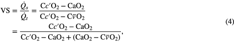
where CxO2 is the oxygen content of blood, Cc'O2 the end-capillary content, and typically (CaO2–C O2) = 5 ml/100 ml of blood. CxO2 can be obtained using

where typically the oxygen-combining capacity of hemoglobin in blood is 1.34 ml O2/(g Hb), Hb = 12 g/100 ml is the hemoglobin concentration in blood, SxO2 is the oxygen saturation, 0.003 is the solubility of O2 in Hb in  .
.
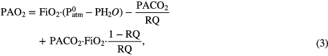
VS is important to the clinician as its magnitude describes the efficiency of gas exchange in the patient which would represent the severity of the underlying pathological disease process. Therefore, we use VS as an output variable that is estimated by the mathematical model. Since equations (4) and (5) can only be solved numerically, this may be inefficient to apply to a pulse oximeter. An alternative is to use P[A-a]O2 as an estimate of VS with the inherent limitations of using partial pressure rather than oxygen content. This measure describes the gradient of PO2 due to the underlying pathology and can be easily displayed in a oxygen cascade (figure 2). When calculating VS, PaO2 is not estimated from FiO2 but from SaO2.
Hill's equation has been modified by Severinghaus to calculate SxO2 from PxO2 (Severinghaus 1979):

The Severinghaus–Ellis equations (Severinghaus 1979, Ellis 1989) allow for the conversion of SxO2 to PxO2:

where


Equations (6) and (7) describe the nonlinear S-shaped Hb–O2 dissociation curve in both directions (figure 3). As the term A of equation (8) is not defined for SxO2 = 100%, we replaced 100% with 99.9% in our model calculations.
Figure 3. The Hb–O2 dissociation curve describes the non-linear relationship between PxO2 and SxO2 and is obtained using the Severinghaus–Ellis equations. This characteristic is largely due to a change in O2 affinity for hemoglobin.
Download figure:
Standard image High-resolution imageIn clinical practice SaO2 is either obtained by analyzing an arterial blood sample in a blood gas analyzer or when not available, estimated using SpO2 from the pulse oximeter reading. The ARMS error in this SaO2 estimation (as illustrated in figure 1) is propagated in our model using the Severinghaus–Ellis equation (7). The pulse oximeter can be considered as an additional stage in the oxygen cascade and SpO2 is used as an input variable that can be measured in the clinical setting (figure 2).
2.2. Experiments
After obtaining ethics approval and written consent, 19 healthy non-smoking subjects (11 males, eight females, median age 28, range 19–50 years) with no history of cardio-respiratory or neurological disease were recruited for a controlled desaturation study. The primary aim of the study was to record data for calibration experiments of a novel mobile phone pulse oximeter using a camera (Karlen et al 2012). The subjects were invited to the physiology laboratory where they rested for 5 min and then underwent a health check by measuring baseline blood pressures, heart rate and SpO2. Fitzpatrick Skin Phototype (Fitzpatrick et al 1988) was assessed (median III, range II–V). Following the successful health check, the study sensors were applied and recording initiated. After 20 min of recording at sea level (FiO2 = 21%), each subject entered a normobaric hypoxia chamber with a FiO2 set to 12%. The FiO2 was then increased stepwise to 17% and then again reduced to 12% (figure 4). After approximately 2.5 h in the chamber, when an FiO2 = 12% was attained and maintained for 5 min, the subjects exited the chamber and were monitored for another 20 min at FiO2 = 21%.

Figure 4. Sequence of FiO2 changes in the hypoxia chamber during the experiment. Duration is approximate as stabilization of FiO2 is dependent on subject in chamber. The blue bold lines depict the data collected for the analysis in this manuscript.
Download figure:
Standard image High-resolution imageThe study sensors consisted of four pulse oximeters that recorded reference data simultaneously. Both, the dominant and non-dominant hands of each subject were fitted with a Nonin Xpod 16 bit (NON, Nonin Medical Inc, Plymouth, USA) and a Masimo Low Power Module (MAS, Masimo Corp, Irvine, USA) oximeter module and finger probe, each connected to a Phone Oximeter on an iPod Touch (Apple Inc, USA) (Karlen et al 2011). The devices recorded a photoplethysmogram (16 bit; MAS 62.5 Hz, NON 75 Hz), heart rate (1 Hz), and SpO2 (1 Hz). They were configured to calculate SpO2 over an average of 8 beats for NON and 8 s for MAS respectively. Both brands of pulse oximeters also provided indicators of artifacts, low perfusion and sensor problems. The sensor data sheets reported an ARMS of ± 2 digits for NON and ± 2% for MAS under conditions without artifacts. Inspired and expired O2 and CO2 and respiratory rate were recorded using Datex-Ohmeda S5 Collect (GE Healthcare, Fairfield, USA) hardware and software at 1 Hz. All recording devices were synchronized to a common time server and a marker was pressed at the beginning of the experiment to verify synchronization.
All data from the reference oximeters on the non-dominant hand and the gas monitor were paired for this study. The data from the dominant hand were not used as they were subject to an increased level of artifacts that would potentially contaminate the data for the purposes of this study. Data pairs labeled with an artifact, low perfusion (MAS perfusion index <1 or >18, NON 'red' perfusion) or sensor warnings of either oximeter were eliminated. The first three minutes after entering or exiting the chamber and after changing FiO2 inside the chamber, where subjects were exposed to large changes in FiO2 in a short period of time, were also discarded to eliminate variations in response time effects of the oximeters and individual subjects physiology.
The distribution of the SpO2 values for a given pulse oximeter at an FiO2 of 21% ± 0.3 and 17% ± 0.3 were plotted as histograms for each device. The 17% threshold was chosen as a second level because it provided the second largest count of data pairs and contained the data with least adaptation effects (changes in respiratory rate and end tidal CO2). Also, the expected SpO2 for this FiO2 is in the range of 93–94%, which coincides with the commonly used threshold for clinical decision making. It was therefore particularly interesting to analyze pulse oximeter tolerance for that range. The standard deviation (SD) for all subjects and the mean of the intra-subject standard deviation (iSD) were calculated. iSD is a more conservative measure as it disregards inter-subject variations that might be present due to sensor placement, perfusion, physiology or other reasons that would lead to measurement variations between observations in different subjects. The obtained distributions were compared with the probability density functions obtained by the model for an 'ideal' pulse oximeter with ARMS = 2% . The probability density functions were plotted for subjects with VSs of 0%, 2% and 5%, all considered normal levels.
3. Results
Propagation of the ARMS through the Severinghaus-Ellis equations (7) and (8) reveals that due to the non-linear relationship of SaO2 and PaO2 the effect of pulse oximeter tolerance is more important at higher SpO2 (figure 5, top). Above SpO2 = 95%, the spread of PaO2 is so large that based on a single observed SpO2, estimation of PaO2 is highly unreliable. In contrast, the tolerance does not cause a large variation in the estimation of VS (figure 5, bottom).

Figure 5. The simulated relationship between oxygen saturation measured by pulse oximetry (SpO2) compared to systemic arterial oxygen partial pressure (PaO2, top) and virtual shunt (VS, bottom). The scatterplots were obtained by applying the Severinghaus–Ellis equation to the simulated data from figure 1. An approximately logarithmic relationship between measured SpO2 and estimated PaO2 was obtained. Pulse oximeter tolerances had a greater effect on PaO2 at a high SpO2 due to the flat shape of the Hb–O2 dissociation curve in this range (94–100%). This effect is reduced in the calculation of VS, since the tolerances of the pulse oximeter only apply to the dissolved oxygen portion of the shunt equation. The pulse oximeter tolerances (confidence intervals of accuracy) are represented by the green (68%) and red (95%) lines.
Download figure:
Standard image High-resolution image3.1. Oxygen cascade model
The oxygen cascade predicts the maximal PaO2 for a healthy subject at FiO2 = 21% (figure 6). The maximal PaO2 with a VS of 0% (PAO2 = PaO2) and FiO2 = 21% was 98 mmHg (13 kPa) at sea level and consequently, when the Severinghaus–Ellis equations were applied, the SaO2 was 97.8% . The oxygen cascade demonstrates that PAO2 increases linearly with an increase in FiO2. PaO2 estimated from SpO2 showed a non-linear relationship characterized by the Severinghaus–Ellis equations and PaO2 estimates. Due to the precision of pulse oximeters, depicted in green (68% percentile) error bars, the estimated PaO2 can be larger than the maximal possible value (PAO2) and consequently VS is negative. The graph in figure 5 allows for an estimate of the likelihood of a shunt for a given SpO2 observation. For example, a measured SpO2 of 94% (black filled dot) has an 84% confidence to have a VS between 7.5% and 19%.

Figure 6. Oxygen cascades for FiO2 = 21% (left) and 17% (right) obtained from our theoretical model showing PxO2 for the inspired, alveolar and arterial stages at a virtual shunt (VS) of 15% (black). The horizontal dashed lines represent alternative PaO2 for VS = 0%, 2% and 5% respectively. The pulse oximeter (with ARMS = 2%) stage is overlaid over the arterial stage for each VS level. The tolerance intervals of the pulse oximeter, showing the measurement 68% confidence interval (green error bar). High SpO2 values have large tolerance intervals due to flat portion of the Hb–O2 dissociation curve. Independent of FiO2, the confidence interval of the SpO2 reading for VS = 0% overlaps with a potential reading for VS = 15% (the most right SpO2).
Download figure:
Standard image High-resolution image3.2. Experiments
A total of 32 672 sample points were obtained for FiO2 = 21% and 6085 for FiO2 = 17% (table 1). The SpO2 distributions were different for the two pulse oximeter brands at FiO2 = 21% (figure 7) and FiO2 = 17% (figure 8). Both sensors were within range when comparing the reported SD and iSD values to the specified accuracy in the respective data sheet. SD was larger than iSD in all situations (table 1), indicating variability between individual subjects. This variability can be also observed in figure 8 where a second peak in the NON distribution can clearly be identified. This variability was also present for the FiO2 = 21%, but was not sufficiently large to produce a secondary peak. There was a clear bias of 1.2% between the oximeters at an FiO2 = 21%, which increased to 2.1% at an FiO2 = 17% (table 1).

Figure 7. Comparison of probability density functions of the model with the empirical distributions of pulse oximeter readings for FiO2 = 21% . Empirical data was obtained for two pulse oximeter brands, NON (blue) and MAS (black), recording from 19 subjects at rest at sea level. Probability density functions for a pulse oximeter with ARMS = 2% were calculated for virtual shunts (VS) = 0, 2, and 5% (red dashed and dotted lines). The pulse oximeters distributions from both devices fit within the theoretical distributions, despite the fact that there is a visible bias between the two empirical distributions.
Download figure:
Standard image High-resolution image
Figure 8. Comparison of probability density functions of the model with the empirical distributions of pulse oximeter readings for FiO2 = 17% . Empirical data was obtained from two pulse oximeter brands, NON (blue) and MAS (black), from 19 subjects at rest in a normobaric hypoxia chamber. Probability density function for a pulse oximeter with ARMS = 2% were calculated for virtual shunts (VS) = 0, 2, and 5% (red dashed and dotted lines). Pulse oximeters distributions from both devices fit within the theoretical distributions, despite the fact that there is a visible bias between the two empirical distributions.
Download figure:
Standard image High-resolution image
Table 1. The distributions of oximeter measurements obtained from the hypoxic chamber experiments.
| FiO2 (%) | SpO2 (%) | HR (beats/min) | n |
||||||||||
|---|---|---|---|---|---|---|---|---|---|---|---|---|---|
| NON | MAS | NON | MAS | ||||||||||
| Mean | SD | iSD | Mean | SD | iSD | Bias | Mean | SD | Mean | SD | Bias | ||
| 21 ± 0.3 | 96.7 | 1.2 | 0.8 | 97.8 | 1.1 | 0.7 | 1.2 | 73.3 | 9.8 | 73.1 | 9.9 | −0.3 | 32 672 |
| 17 ± 0.3 | 93.2 | 1.7 | 1.1 | 95.4 | 1.4 | 1.0 | 2.1 | 72.4 | 9.5 | 72.1 | 9.5 | −0.3 | 6085 |
aThe samples are not statistically independent as averaging is used during sampling. Note: Blood oxygen saturation (SpO2) and heart rate (HR) was collected for two inspired gas fractions (FiO2) and two pulse oximeter brands (NON and MAS). Mean, standard deviation (SD) and bias between oximeters were calculated for n data pairs combined from the 19 subjects. The mean from the intra-subject SD (iSD) is also reported. iSD is more accurate than SD in describing the sensor tolerance.
4. Discussion
We have described a model to estimate VS from FiO2 and SpO2. The model facilitates the analysis of effects of variability in pulse oximeter readings due to tolerances in the SaO2 estimations. An improved clinical understanding of the limitations of pulse oximetry will promote improved clinical decision making.
The VS has been used as estimate of the pathological severity of an impairment of oxygen delivery. This theoretical concept describes the overall loss of O2 content between the alveolar gas and arterial blood. Estimating VS is of clinical importance as its magnitude can be used to estimate disease severity and, more importantly, to track the progression of the process over time. It can also be used to optimize therapies such as ventilation and oxygen administration. However, measuring VS directly is not clinically practical. Typically, graphs containing iso-shunt lines are used by clinicians to estimate VS based on known FiO2–PaO2 relationships (Benatar et al 1973). Alternatively, VS has been modeled in a computer simulation and can be estimated by entering FiO2–PaO2 pairs into the software interface (Kretschmer et al 2013). Exact PaO2 is available through blood gas analysis, which can only be accessed with delays at discreet time intervals. A potential application of pulse oximetry would be to indirectly estimate the magnitude of VS continuously by estimating SaO2 and PaO2. Our model expands the concept of PiO2 versus SpO2 diagrams (Sapsford and Jones 1995) by displaying pulse oximeter tolerances. The concept of tolerance intervals has been used since the beginning of pulse oximetry to describe the accuracy and limitations of pulse oximeters (Wukitsch et al 1988). However, it has rarely been used for direct display in oximeters or estimations of shunt.
The simulated experiments show that the non-linearity of the Hb–O2 dissociation curve (figure 3) cause large effects in the PaO2 estimation at high SpO2 when taking pulse oximeter tolerance into account. This high variability in estimated PaO2 over a short range of SpO2 can be misleading due to the flat portion of the Hb–O2 dissociation curve. However, since the reported error rate of pulse oximeters do not vary over a larger range (typically 80–100%), the estimation of PaO2 from pulse oximeter readings becomes more accurate at a lower SpO2. In an analogous situation, a small change in the oxygen saturation on the flat portion of the oxygen dissociation curve would indicate a much bigger change in PaO2 than the same amount of change at a lower saturation. The true 2% change in SaO2 in the high nineties indicates a much more significant change in pathology than the 2% change in the patient with a SaO2 in the low eighties. The effects on the estimation of VS is more linear than PaO2 (figure 5). This is explained by the fact that the tolerances of the pulse oximeter only apply to the dissolved oxygen portion of the equation. However, the model shows that large oximeter tolerances can cause variations of up to 25% at a SpO2 = 94%.
From the theoretical models it becomes clear that at sea level, an SaO2 of 98% and higher is only possible if O2 is administered. The experimental data confirmed this, with peaks in the SpO2 distribution at 98% (MAS) and 97% (NON). At this altitude, an ideal pulse oximeter with ARMS = 2% could display any SpO2 between 96% and 100% at a 68% tolerance interval or 94–100% at a 95% tolerance interval. This corresponds to a maximal estimated VS of 7.5% and 14% respectively. To produce an SaO2 of 100% in a patient at sea level, the administration of at least 47% O2 would theoretically be required.
An increase in bias for SpO2 values lower than 95% between oximeters has been previously observed (Van de Louw et al 2001). Both tested sensors were within tolerance specified in their data sheets when comparing the reported values to the theoretical values of an ideal oximeter that complies with ISO standards. NON reported more conservative SpO2 values than the MAS, suggesting a larger VS (≈5%). The distribution of MAS values was very close to the theoretical maximum achievable SpO2, corresponding to a VS = 0% suggesting that this type of sensor may be overestimating SaO2.
Our theoretical and practical findings show that the accurate estimation of PaO2 and VS is challenging with a single SpO2 measurement as the tolerance of pulse oximeters is relatively large (ARMS = 2%). An oxygen cascade graph can easily illustrate this inaccuracy and the effect on VS estimation (figure 6). Oximeter readings suggesting a VS of 0% cannot exclude a VS of 15% at the 68% confidence interval. This uncertainty may be reduced with collecting multiple independent samples (ideally under different conditions) that will describe an SaO2 distribution. Changing conditions can be produced in various ways. To establish their model, Kjaergaard et al (2003) administered O2 to patients to obtain a variation in exhaled O2 and subsequently calibrate the model. In addition they relied on a invasive blood sample to calibrate for Hb and pH. As these invasive measures were not available in our setting, we relied on multiple observations of the same subject state with two independent oximeters. These observations result in a distribution with the mean describing the most likely estimation of SaO2. Such an approach is already practiced with automated blood pressure devices that repeat measurements 3–5 times and report an average to minimize measurement error and white-coat effects (Myers 2006). However, the use of multiple measurement points of a continuous time series, without replacing or relocating the oximeter probe (as performed with the blood pressure device) would not reduce the overall error. Pulse oximeters use an internal, proprietary averaging algorithm making measurements dependent on previous samples. Collecting multiple SpO2 samples is already manually performed in practice when the measurement procedure is repeated with repositioning or placement of a different sensor. This is produced when the results of the initial measurement do not seem plausible, e.g. when the user suspects an incorrectly placed or defective probe. However, there is a need for performing this measurement repetition in a more systematic way which needs further investigation. In addition, the method for merging the observations (i.e. mean or median) and the number of multiple, consecutive SpO2 measurements required to provide the best estimate of SaO2 with higher accuracy needs investigation. Finally, technical improvements in the oximeter device itself could provide direct guidance for the need to repeat the measurements at specific intervals and sensor locations.
4.1. Limitations
In this work, a number of co-variates in the model such as Hb and PxCO2 were kept invariant. While our physiological models would allow these parameters to be included as variables in the theoretical calculations, exact values are not available in clinical practice without invasive sampling and were also not available during our experiments. Our model consists of a single compartment to estimate VS. More precise models, for example with two (Karbing et al 2011, Kretschmer et al 2013), three (Jones and Jones 2000, Karbing et al 2011) and five (Wang et al 2010) compartments, have been suggested. However, considering the shown tolerance effects of pulse oximeters on the models overall accuracy, the increased complexity of higher compartment order is unlikely improving VS estimations in practice.
A low PaO2 triggers a physiological response that compensates for the reduced O2 intake during breathing of hypoxic gas mixes. A short term adaptation is the increase of respiratory drive and consequent reduction of PACO2. This is a typical adaptation to higher altitudes and is also observed in our data. PACO2 and all other CO2 partial pressures will decrease immediately at exposure causing a left shift of the Hb–O2 dissociation curve and a relative increase in PAO2. This could not be avoided during data collection, but was minimized by using data for analysis that was collected after the typical short term adaptation period of 3 min. The longer term (multiple hours/days) adaptation process of increasing the concentration of 2,3-diphosphoglycerate leading to a right shift of the Hb–O2 dissociation curve and lowering the O2 affinity (West 2012) was considered negligible due to the short duration of our experiments.
For this study, arterial blood gas samples were not available to confirm the estimated SaO2. We can therefore only speculate about the real PaO2 and VS that the subjects experienced during the experiments. This corresponds to many clinical situations where arterial sampling of blood gases is not immediately available or desirable.
5. Conclusion
We have illustrated the propagation of pulse oximeter tolerance from the measurement of SpO2 to the estimation of VS. Theoretical and experimental results show that the effect is amplified at higher SpO2 readings. The findings show that the estimation of PaO2 and VS should ideally not be made from a single SpO2 observation. To reduce tolerance effects and artifacts due to aberrant oximeter readings in the clinical setting we recommend performing multiple observations of SpO2 before undertaking critical clinical decisions.
Acknowledgments
The authors are grateful to Prof M Koehle, Prof J Rupert and M MacInnis at the School of Kiniesology, The University of British Columbia, Vancouver for making the hypoxia chamber available for our research and all volunteers that participated in the experiments. We are also thankful to Dr H Gan, D Meyers, and A Umedaly who kindly helped us in conducting the data collection for this study. This work was financially supported in part by Grand Challenges Canada (CRS2_0041) and the Swiss National Science Foundation (PA00P2_136454).