
Abstract
In this work, we demonstrate the use of the Green–Kubo integral of the heat flux autocorrelation function, incorporating long-range corrections to model the thermal conductivity versus temperature relationship of cross-linked polymers. The simulations were performed on a cross-linked epoxy made from DGEBA and a curing agent (diamino diphenyl sulfone) using a consistent valence force field (CVFF). A dendrimeric approach was utilized for building equilibrated cross-linked structures that allowed replication of the experimental dilatometric curve for the epoxy system. We demonstrate that the inclusion of a long-range correction within the Ewald/PPPM approach brings the results close to experimentally measured conductivity within an error of 10% while providing a good prediction of the relationship of thermal conductivity versus temperature. This method shows significant promise towards the computation of thermal conductivity from simulations even before synthesis of the polymer for purposes of materials by design.
Export citation and abstract BibTeX RIS
1. Introduction
Manufacturers are constantly in search of new and better epoxies to improve heat conduction in composites in order to remove excess heat and boost reliability and performance. The range of temperatures at which these polymers operate may be quite large and it is important to model the relationship of thermal conductivity with temperature. Atomistic simulation methods have the potential to replace costly experimentation when identifying such relationships for the purposes of material selection. In this work, we study the use of the Green–Kubo integral [1] of the heat flux autocorrelation function to model the thermal conductivity versus temperature relationship of cross-linked epoxies.
One of the key challenges in the molecular simulation of industrial epoxies is the attainment of sufficient cross-link conversion so that its properties are well represented. Epoxies used in industrial prepegs display 70–95% cross-link conversion when measured through near-infrared (NIR) spectroscopy [2]. Most of the approaches used in the past to achieve over 70% cross-link conversion involve the process of polymerizing unreacted monomer mixtures either over time (multi-step) or all at once (one-step). In one-step cross-linking [3, 4], cross-linking sites are randomly selected and pairs of sites within a capture radius are cross-linked together. One-step methods lead to artificially high network strains. In multi-step cross-linking [5–7], all reactive pairs that satisfy a given length criteria are cross-linked. The length criteria increases with each iteration and equilibration and cross-linking are repeated until the desired cross-linking density is reached. Although multi-step methods prevent and relieve network strains, these are computationally intensive. Christensen [8] introduced a new method to build epoxy networks using a 'dendrimer' growth approach. In this approach, the thermoset resin is modeled by starting with a single monomer and then cross-linking a second layer of monomers around it. In the next step, a third layer of monomers is cross-linked to the second layer. In this way, generations (layers) of monomers are added to a seed structure that grows in size at every pass. The principal advantages of the dendrimer growth method are the complete avoidance of artificial network strain during curing and the low computational cost of the growing procedure. Figure 1 shows a three-dimensional (3D) dendrimer used to build the molecular model of a cross-linked epoxy structure. This approach is studied in this work for building realistic energy-minimized polymer unit cells and for the computation of thermal conductivity.

Figure 1. 3D dendrimer used to build the molecular model of a cross-linked epoxy structure.
Download figure:
Standard image High-resolution imageAlthough MD simulations have been used in the past to study thermal properties, most of these studies have focused on simpler materials such as metals, ionic salts and non-cross-linked polymers [9–11]. Only recently has the thermal conductivity of cross-linked polymers been studied through such approaches [12]. The calculation for thermal conductivity has traditionally been performed using either equilibrium MD (within the Green–Kubo formalism [1]) or using non-equilibrium MD approaches ([13]). In the latter methods, a long polymer slab is built and a temperature difference (or a heat flux in reverse NEMD [14]) is established between a heat source and sink at the ends of the slab, and the flux (or temperature difference) is calculated. Green–Kubo approaches are well suited when using a dendrimeric polymer builder that naturally builds cubic unit cells rather than the elongated slabs needed for NEMD approaches. In addition, a comparison between the NEMD method and Green–Kubo's equilibrium approach was previously performed by Varshney et al [12] for an epoxy structure built using a multi-step reaction method, and these two methods were found to result in similar values of thermal conductivity.
Equilibrium MD simulations were performed using the dendrimer structure and the heat flux autocorrelation function was computed at different temperatures. The expression for the heat flux appearing in the integrand of the Green–Kubo formulation for thermal conductivity is well known for the systems with short-range pair interactions, such as the Lennard–Jones or the embedded atom potential. In cross-linked polymers, the interatomic interactions are long range due to the presence of electrostatic forces between partial charges on atoms. The per-atom energy needed for the computation of the heat flux vector in this case is more conveniently calculated on a periodic domain using the Ewald or PPPM methods [15]. Here, the 'real-space' component of electrostatic energy is computed within a small cut-off distance while the 'reciprocal' or 'k-space' part that decays with the inverse distance is used to handle the slow decay beyond this distance. We employ this approach to find the thermal conductivity of di-glycidyl ether of bisphenol A (DGEBA)/diamino diphenyl sulfone (DDS) resin for various minimized configurations. The thermal conductivity with and without long-range corrections are compared to experimental results reported in the literature to illustrate the importance of long-range interactions in determining thermal conductivity. The conductivities are computed as a function of temperature for two resin materials: DGEBA/33DDS and DGEBA/44DDS. The conductivity of Polymethyl methacrylate (PMMA) is also computed to serve as a lower bound, since it is known that its conductivity is lower than the epoxies considered. The remainder of this work is organized as follows. In section 2, the dendrimer approach for building a thermally equilibrated epoxy structure is discussed. In section 3, the Green–Kubo approach for thermal conductivity calculation including methods to compute the effect of long-range electrostatic interactions in reciprocal space is discussed. In section 4, the convergence of the Green–Kubo approach is discussed and the calculated thermal conductivities for epoxy and PMMA as functions of temperature are compared with experimental results.
2. A dendrimeric model of epoxy
For this study, a common epoxy was employed: DGEBA. The epoxy and amine monomer structures are shown in figure 2. The epoxy molecules were cross-linked (cured) with DDS. Each epoxy monomer has two epoxide (oxirane ring) groups, each with a cross-linking functionality of one towards amine curing agents, for a total functionality of two; each DDS monomer has two amine groups, each with a functionality of two towards epoxy molecules, for a total functionality of four. The typical synthetic epoxy to amine stoichiometric ratio is approximately 2 : 1 or 33.3 mol% amine [16]. Figure 3 shows polymer formation driven by the bonding of the epoxide group in DGEBA and the amine groups in DDS. During the formation of a cross-link, the primary amine group reacts with the epoxide group, forming a bond between the nitrogen of DDS and the terminal carbon of the epoxide group. The carbon–oxygen bond breaks between the terminal carbon and the epoxide oxygen to form an alcohol (–OH) link. The cross-linked structure in figure 3(a) can undergo further reaction with another epoxy molecule to form a cross-linked molecular structure (figure 3(b)).
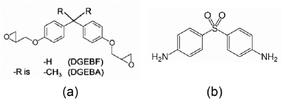
Figure 2. Chemical structure of epoxy resin monomer units. DGEBA and the amine monomer 4–4' diamino diphenyl sulfone. In 3–3' diamino diphenyl sulfone (not shown here), the two amine groups are instead attached to the next neighboring carbon atom in the ring.
Download figure:
Standard image High-resolution image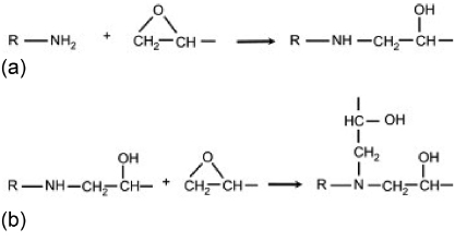
Figure 3. Epoxy-amine cross-linking through the reaction of the amine group with the epoxide group.
Download figure:
Standard image High-resolution imageWe have used the 'dendrimer' growth approach introduced in [8, 24] to build epoxy networks in Materials Studio by Accelrys Software Inc [17]. In this approach, the epoxy and amine monomers are first built and the atoms in the monomers that cross-link are marked as 'connect atoms'. The model starts with a single seed monomer (epoxy unit). The 'dendrimer' build function in Materials Studio is instantiated to cross-link amine units to this seed. This forms the first generation of the dendrimer. The dangling 'connect atoms' from the amine units of the first generation are then bonded to a new set of epoxy units in the second generation of the dendrimer. The procedure is repeated until a sufficiently large dendrimer is obtained. The approach is described in greater detail in [24]. The dendrimers are inserted in periodic cubic cells using the Amorphous Cell module in Materials Studio and are initially constructed at a low density of 0.4 g cm−3 and at a temperature of 650 K. While the dendrimer itself is a self contained unit, when it is minimized in the cubic cell, the polymer is wrapped around the periodic boundaries, which leads to a fully condensed system with interactions across the 3D cell boundaries. The cubic cell is then annealed using the Discover module in Materials Studio to generate equilibrated structures at ambient conditions. The temperature for all simulations was equilibrated with the Andersen thermostat [18] and the applied pressure for the isobaric simulations was controlled with the Andresen barostat [18]. The sample is cooled down to 300 K in steps of 50 K; at each temperature, a 50 ps long simulation at constant volume and temperature (NVT ensemble) was performed followed by a constant pressure and volume (NPT) run for an additional 50 ps. As described in table 1 (from [24]), the pressure is increased during the annealing process to achieve compaction. After annealing, the energy-minimized periodic cells were then used as a starting point for a 250 ps production run using NPT dynamics at one atmosphere with periodic boundary conditions. A snapshot of the trajectory was stored every 2.5 ps. The last ten frames of the trajectory were then examined and the structure with the highest density was selected for an analysis of the properties. For equilibration simulations, the COMPASS forcefield was used [20]. For all the thermal conductivity simulations presented in this study, the consistent valance force field (CVFF) potential [21] was used for bonded as well as non-bonded interactions within LAMMPS [22]. This force field successfully predicted accurate thermodynamic properties of interest for epoxies in a previous study [6]. To compare the properties of the epoxy with experimental dilatometric data [23], the minimized cell was subject to NPT simulations at various temperatures. The change in cell length with temperature is superposed with the experimentally measured dilatometric curve reported in [23] in figure 4 and the data show good agreement. The linear coefficient of thermal expansion between 223 to 323 K is measured to be 54.6 μ/K from this figure.

Figure 4. (a) The dendrimer structure of epoxy after energy minimization. (b) MD calculations of thermal expansion is superposed with the experimentally measured dilatometric curves reported in [23].
Download figure:
Standard image High-resolution imageTable 1. Annealing protocol for building the equilibrated epoxy structure.
| NVT for 50 ps at 650 K (equilibration) |
| NPT for 50 ps at 650 K and 0.1 GPa (initial compaction) |
| NVT for 50 ps at 500 K (equilibration) |
| NPT for 50 ps at 500 K and 0.25 GPa (additional compaction) |
| NVT for 50 ps at 450 K (equilibration) |
| NPT for 50 ps at 400 K and 0.0001 GPa (reduce to 1 atm) |
| NVT for 50 ps at 300 K (equilibration) |
| NPT for 50 ps at 300 K and 0.0001 GPa (equilibration) |
| Minimization |
In the initial dendrimer (see figure 4(a)), 75% of the available epoxy sites were cross-linked, which is representative of many structural epoxies [2]. The use of small four to six thousand atom systems was motivated by the fact that all simulations in this work are performed under periodic boundary conditions and the representative epoxy structure provided the sufficient complexity needed to capture the amorphous nature. The correctness of the representation was studied by comparing the dilatometric curves predicted by MD with experimental results (figure 4). The conductivity of a PMMA structure is also computed to serve as a lower bound value. For the PMMA structure, the dilatometric curve was computed and the coefficient of linear thermal expansion was found to be 68.33 μ/K, which compares well with the experimental range of 65–70 μ/K. Two different structures were tested: DGEBA/33DDS and DGEBA/44DDS, with multiple instantiations for each polymer to test the variability in conductivity. Table 2 gives the simulation cell specifications for the epoxy and PMMA unit cells.
Table 2. Specification of molecules.
| Structure | No of atoms | Dimensions (A3) | Density (g cm−3) |
|---|---|---|---|
| DGEBA-DDS | 4562 | 36.01 X 36.01 X 36.01 | 1.17 |
| PMMA | 5768 | 39.42 X 39.42 X 39.42 | 1.05 |
3. Green–Kubo method for predicting thermal conductivity
The Green–Kubo method is an equilibrium MD approach that relates the fluctuations of the heat current along a direction, Jx, to the thermal conductivity (K) via the fluctuation-dissipation theorem [1, 25]. The thermal conductivity is given by

where 〈Jx(t)Jx(0)〉 is the heat current auto correlation function (HCACF). V and T represent the volume and temperature of the system, respectively, while kB is the Boltzmann constant.
In general, the conductivity is averaged across all three directions to obtain the scalar conductivity of an isotropic material. For the present study, the following formula is employed with a factor of three in the denominator denoting an average across x, y and z directions and J is the heat flux vector:

In the above expression, tc stands for a finite correlation time for which the integration is carried out and ts stands for the sampling time over which the ensemble average for computing HCACF is accumulated.
There are multiple ways to define the heat current vector [26]. The most commonly used definition is
where ri and ei are the position vector and total energy of atom i, respectively, and the summation is over the total number of atoms (N) in the system. The energy of atom i(ei) is given as the sum of the potential energy (PE) and kinetic energy (KE):

where mi and vi represent the mass and velocities of atom i. The potential energy of atom i(Ui) depends on the form of the interaction potential (includes bonded and non-bonded interactions) employed in the simulations. In the CVFF potential, the total energy is computed as a sum of pair interactions (Upair), coulombic interactions (Ucoulomb) and energies that account for changes in bond lengths (Ubond), bond angle (Uangle), dihedral angle (Udihedral) and improper dihedral angle (Uimproper) in the following form:

The per-atom energy (Ui) is computed by averaging the energy contributions in equal portions to each atom within an interaction set. For example, a quarter of the dihedral energy is assigned to each of the four atoms involved in the dihedral term.
The first term is a pairwise energy contribution where n loops over the Np neighbors of atom i, and ri and r2 are the positions of the two atoms in the pairwise interaction. The second term is a bond contribution of a similar form for the Nb bonds which atom i is part of. There are similar terms for the Na angle, Nd dihedral and Ni improper interactions that atom i is part of. Note that the Ucoulomb contribution from long-range Columbic interactions is handled differently using an Ewald summation and is described separately in the next section.
By substituting equation (4) into equation (3) and performing differentiation with respect to time, the microscopic heat current vector J is obtained as
Here, Si denotes the per-atom stress tensor as defined below. The first term on the right-hand side represents the diffusive part of the heat flux, i.e. the contribution of atomic motion to energy transport. The second term on the right-hand side is the interaction part of the heat flux representing the contribution of interactions to the transfer of energy. When using the CVFF potential, the stress tensor for atom i (Si) is given by the following formula, where a and b take on the values x, y, z to generate the six components of the symmetric tensor:
In the first three terms, Fi and F2 are the forces on the two atoms resulting from their interaction. There are similar force terms for the angle, dihedral and improper interactions of atom i. Note that the above stress tensor only contains the virial terms and does not include the kinetic energy contribution.
3.1. Computation of long-range coulombic interactions
In cross-linked polymers, the interatomic interactions are long range due the presence of electrostatic forces between the partial charges on atoms. The per-atom energy needed for the computation of the heat flux vector in this case is more conveniently calculated on a periodic domain using the Ewald or PPPM methods. Here, the 'real-space' component of electrostatic energy is computed within a small cut-off distance while the 'reciprocal' or 'k-space' part that decays with the inverse distance is used to handle the slow decay beyond this distance. The Ewald expression for potential energy Ucoulomb and its contribution to the stress tensor are computed in this section. In the Ewald approach, the electrostatic potential energy of a neutral distribution of N atoms with point charges qi can be written as [27]
In equation (9), rij = |rj − ri| is the distance between charges i and j, and erfc(κ rij) in the first term on the right-hand side is the complimentary error function of the distance multiplied by a convergence factor κ, and the second term on the right-hand side is the Fourier expansion of the difference between the first term and the full electrostatic potential energy. The Fourier expansion in terms of wave vectors kα = (2πnα/L) (α = x, y, z) is used where L is the periodic box size. Also,  0 is the electric permittivity of free space.
The k-space part of the electrostatic potential energy and the stress tensor, in addition to a sum over wave vectors k, contains double sums over all of the pairs of atoms i, j; i ≠ j. Observing that rij = rj − ri, this double sum can be written as a single sum over N charges, which speeds up the computation by N-fold [28].
Here, S (k) is the structure factor given as
 . The sum of the squared charges is subtracted because the first term on the right-hand side contains the self-interaction term with i = j. With the use of the transformation (10), the expression for the electrostatic potential energy is
The subtracted term
 , corresponding to i = j, is the contribution due to self-interaction. The per-atom version of the potential energy contribution is calculated using a per-atom structure factor Θi(k) defined as Θi(k) = qi exp(ik.ri) as follows:
The elements of the coulombic part of the stress tensor are obtained by the differentiation of equation (11) with respect to the components of rij. The resulting electrostatic part of the stress tensor (Sab)coulomb is given as follows, where a and b take on the values x, y, z to generate the six components of the symmetric tensor [29]:
where δαβ is the Kroneckar symbol. The per-atom stress tensor is computed using the per-atom structure factor as
The PPPM solver employs the same approach as the Ewald approach described above, except that atomic charges are mapped to a 3D mesh and FFTs are used to compute the structure factors.
4. Simulation results
In the initial convergence studies, a Lennard–Jones/Coulomb interaction cutoff of 12.5 Å (about 30% of the box length) was used without the Ewald approach. The original dendrimer was optimized at room temperature. In order to compute the thermal conductivity at different temperatures, NPT ensemble molecular dynamics simulations were performed for 0.1 ns (at 1 atm pressure) to get the equilibrium structure at that particular temperature, and then further equilibration was carried out over longer times to collect heat flux data that was used to calculate the autocorrelation function. Convergence of HCACF with the sampling time was subsequently studied and the results are plotted in figure 5 for an epoxy at 223 K. The sampling interval was taken to be the same as the time step (1 fs). The measured HCACF at sampling times between 0.032 and 0.392 ns are compared here. From figure 5(b), it can be seen that HCACF is beginning to show some convergence at 0.392 ns. In addition, we studied the effect of temperature on the convergence of HCACF in figure 6. Here, the convergence error for HCACF is computed by comparing HCACF at the current sampling time ts with HCACF at ts = 0.096 ns. At higher sampling times, HCACF converges and the convergence error flattens out. Figure 6(b) shows the convergence error for temperatures ranging from 223 to 423 K for the epoxy structure. It can be seen that the convergence is faster at higher temperatures. Based on a sampling time of ts = 0.4 ns, we identified the optimal correlation time (tc) for computing thermal conductivity. This was done by plotting HCACF as a function of time (as shown in figure 7 for epoxy at a temperature of 375 K and PMMA at 300 K) where it can be seen that a correlation time of 8 ps is sufficiently large, beyond which HCACF values were insignificant. While a correlation time of 8 ps was subsequently employed to compute the thermal conductivity, the correct sampling time ts itself was later found by observing the convergence of the thermal conductivity with sampling time.
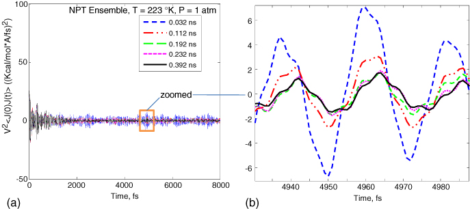
Figure 5. (a) HCACF plotted as a function of sampling time. (b) Zoomed region of the plot in (a) is shown here to show the slow convergence of HCACF.
Download figure:
Standard image High-resolution image
Figure 6. (a) HCACF is plotted as a function of temperature. (b) Convergence of HCACF with sampling time is shown for different temperatures. Convergence is faster at higher temperatures.
Download figure:
Standard image High-resolution image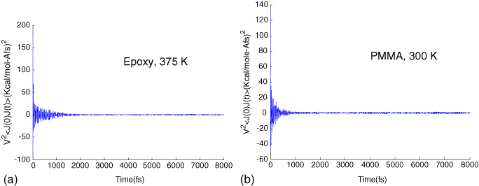
Figure 7. (a) HCACF for epoxy at T = 375 K. (b) HCACF for PMMA at T = 300 K.
Download figure:
Standard image High-resolution imageIn figure 8, we compared the values obtained for thermal conductivity from three different approaches (for epoxy DGEBA/33DDS at 300 K) as a function of sampling time. The first approach was a real-space algorithm that did not include any long-range k-space corrections. The second and third approaches were Ewald and PPPM methods, both including the effects of long-range electrostatic forces as described in section 3. In the Ewald and PPPM approaches, the free parameters, such as the convergence acceleration factor, number of k-space vectors (in Ewald) or grid size (in PPPM), are determined by specifying an accuracy value (see [30, 31]). An accuracy value of 10−4 was specified, which means that the error will be a factor of 10 000 smaller than the force that two unit point charges exert on each other at a distance of 1 Å. All three methods show convergence with sampling times, with convergence seen beyond 1.0 ns (106 time steps). The experimental value of thermal conductivity for epoxy at room temperature is about 0.25 W m−1 K−1 [32]. The use of long-range corrections within Ewald or PPPM approaches allows convergence to a value of thermal conductivity closer to experiments. PPPM and Ewald approaches give almost the same value for thermal conductivity, but PPPM is significantly faster due to the use of fast Fourier transforms and scales with the number of atoms as N log (N) (compared to N3/2 for Ewald). Since the thermal conductivity oscillates over a small range even at large sampling times, the results from the last 0.1 ns of the simulation were averaged to compute the values reported in this paper.
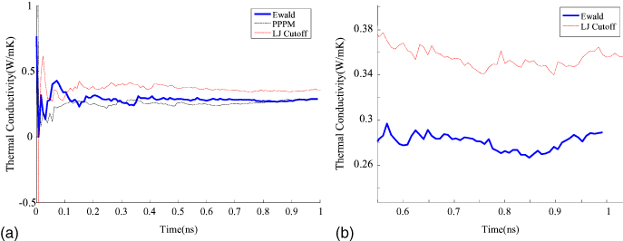
Figure 8. (a) Convergence of thermal conductivity of three methods (Ewald, PPPM and atom-based LJ cutoff) with sampling time (for epoxy, 300 K), zoomed in (b). The addition of a long range coulombic term results in a conductivity closer to the experimental value of 0.25 W m−1 K−1 [32].
Download figure:
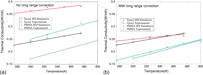
Standard image High-resolution imageThe conductivity of PMMA was also computed to serve as a lower baseline, since it is known that its conductivity is lower than the epoxies considered. In figure 9, we have reported the variation of thermal conductivity with temperature and compared it with the experimental results available in [32]. On the same graph, the thermal conductivity of PMMA is also calculated and is lower than epoxies, as expected. The conductivity of PMMA is also compared with the experimental results in [33]. Two plots are shown: with thermal conductivity computed without long-range corrections as shown in figure 9(a) and thermal conductivity computed including long range corrections using the PPPM approach shown in figure 9(b). The trend of thermal conductivity versus temperature is well captured with or without long-range corrections, with the thermal conductivity increasing with temperature close to the same linear slope as experiments. The thermal conductivities computed without long-range corrections were about 50% higher for epoxies when compared to experiments. The inclusion of long-range corrections within the PPPM approach bring the results closer to experiments with an error as low as 10%. The improvement in results reported here may be due to well equilibrated dendrimeric construction methods employed here that were previously successful in reproducing properties like elastic modulus, thermal expansion and yield strength (in [34]).
Figure 9. (a) Thermal conductivity from MD compared with experiments when using atom-based cut-off. (b) Thermal conductivity corrected for long-range electrostatic interactions compared to experiments.
Download figure:
Standard image High-resolution image
Although this work is performed at the lower end of the cross-link conversion percentage (75%), it is of interest to investigate the effect of a higher cross-linking density on thermal conductivity. Recent work by Kikugawa et al [35] shows that the magnitude of change in thermal conductivity with cross-link density for molecules like polystyrene (with heavier side groups like phenyl) is relatively small. In the dendrimer approach, the outermost non-cross-linked layer reduces the overall cross-link conversion. The manual addition of intramolecular loops to connect unreacted sites has been suggested in the past [16] and could be used in future work to investigate a higher cross-link conversion. In addition, it is also of interest to investigate the sensitivity of the calculated thermal conductivity to the particular dendrimer structure employed. We employed three structures of epoxy/33DDS, epoxy/44DDS and PMMA built using different initial conditions. Specifically, the initial dendrimer cells were independent amorphous cells (leading to different initial atom positions), which has an effect on the final equilibrated network structure. The results are summarized in table 3 with ± data spread accounting for various different dendrimer structures tested for the same polymer resin. The results show that the calculated values of thermal conductivity show low sensitivity to the starting dendrimeric structure, and give similar conductivity values for different equilibrated structures.
Table 3. Thermal conductivity (W m−1 K−1) variation of Epoxy with temperature.
| Structure | 275 K | 300 K | 325 K | 350 K | 375 K |
|---|---|---|---|---|---|
| DGEBA-33 | 0.2403 ± 0.0279 | 0.2510 ± 0.0386 | 0.2603 ± 0.0308 | 0.2628 ± 0.0427 | 0.2624 ± 0.0243 |
| DGEBA-44 | 0.2418 ± 0.0137 | 0.2592 ± 0.0129 | 0.2587 ± 0.0092 | 0.2611 ± 0.0274 | 0.2636 ± 0.0201 |
| PMMA | 0.1651 ± 0.0153 | 0.1834 ± 0.0186 | 0.1933 ± 0.0245 | 0.2186 ± 0.0258 | 0.2357 ± 0.0274 |
5. Conclusions
Epoxies with improved heat conduction have the potential to remove excess heat and boost reliability. Atomistic simulation methods have the potential to replace costly experimentation to identify the thermal conductivity of polymers for the purposes of material selection. In this work, we demonstrate the use of the Green–Kubo integral of the heat flux autocorrelation function incorporating long-range corrections to correctly model the thermal conductivity versus temperature relationship of cross-linked polymers. A dendrimeric approach was utilized to build equilibrated cross-linked structures that allowed replication of the experimental dilatometric curve for the epoxy system. Two approaches for calculating thermal conductivity were studied, one using a large LJ cutoff without Ewald summation and another using the Ewald/PPPM approach where a correction term accounting for long-range coulombic interaction was included. A correlation time of 8 ps and sampling times of 1.5 ns were seen to be sufficient for the convergence of calculated thermal conductivity. As a baseline reference, the computed conductivity of epoxy was compared to PMMA and the values were higher than expected from both methods. The trend of thermal conductivity versus temperature observed from experiments was well captured with or without long-range corrections. However, the thermal conductivities computed without long-range corrections were about 50% higher for epoxies compared to experimental results. The inclusion of long-range correction within the Ewald/PPPM approach brings the results closer to experiments with an error as low as 10% for both PMMA and epoxies. Furthermore, the calculated value of thermal conductivity shows low sensitivity to the starting dendrimeric structure. These results show significant promise for the computation of thermal conductivity from MD simulations even before synthesis of the polymer for purposes of materials by design.