
Abstract
To improve the efficiency of energy harvesting, this paper presents a tri-stable energy harvesting device, which can realize inter-well oscillation at low-frequency base excitation and obtain a high harvesting efficiency by tri-stable coherence resonance. First, the model of a magnetic coupling tri-stable piezoelectric energy harvester is established and the corresponding equations are derived. The formula for the magnetic repulsion force between three magnets is given. Then, the dynamic responses of a system subject to harmonic excitation and Gaussian white noise excitation are explored by a numerical method and validated by experiments. Compared with a bi-stable energy harvester, the threshold for inter-well oscillation to occur can be moved forward to the low frequency, and the tri-stable device can create a dense high output voltage and power at the low intensity of stochastic excitation. Results show that for a definite deterministic or stochastic excitation, the system can be optimally designed such that it increases the frequency bandwidth and achieves a high energy harvesting efficiency at coherence resonance.
Export citation and abstract BibTeX RIS
1. Introduction
Advances in low-power electrical systems in recent decades have led to a greatly increasing requirement for clean alternative power. Environmental energy harvesting has attracted considerable interest because it could directly extract electricity from an ambient source.
In energy harvesting, the most common transduction mechanism is a piezoelectric energy harvester, which converts mechanical dynamic strain into electricity. Various studies of energy harvesting have adopted the linear assumption and exploit resonance to generate the maximum power. However, since an ambient source has a wide spectrum, the linear energy harvester will become incapable of working efficiently [1–3].
To overcome this problem, many methods have been explored by researchers to broaden the bandwidth of a harvester, e.g. oscillator arrays [4] and an active frequency-tuning method [5]. Another significant improvement in broadband performance is achieved by introducing nonlinearity into the design of an energy harvester [6–22]. Numerous nonlinear factors such as mono-stability [6–9], bi-stability [10–15] and impact [16] are introduced to broaden the bandwidth. Gafforelli et al [9] experimentally investigated the mono-stable Duffing nonlinear oscillator with a doubly clamped beam. The results show that the frequency bandwidth becomes significantly wide. The bi-stable energy harvester (BEH) has received much attention due to its high output power when the device snaps through from one stable state to another [8–10]. Stanton et al [13] studied the piezo-magnetoelastic bi-stable energy harvester with magnetic repulsion and provided a mathematical expression for the forces between magnets. Erturk and Inman [14] presented results of a theoretical and experimental investigation of high-energy orbits in the piezomagnetic bi-stable energy harvester over a range of excitation frequencies. Zhao and Erturk [15] investigated the relative advantage of bi-stable and mono-stable energy harvesters under broadband random excitation. Results show that the bi-stable configuration generates more energy when the level of excitation is above the threshold of inter-well oscillation.
Recently, more complex energy harvesting systems composed of a tip mass and multiple external magnets have been proposed, with which the tri-stable mechanism could be realized [17–22]. Kim and Seok [17] considers numerical analyses of bifurcation for the multi-stable mechanism. Zhou et al [18, 19] and Cao et al [20] carried out numerical and experimental investigations on a tri-stable energy harvester (TEH) with two rotatable external magnets under harmonic excitation. Results demonstrate that it can improve the performance and broaden the usable bandwidth. They also discussed the influence of potential well depth and found that a shallower potential well would enhance the capacity for harvesting energy from low-frequency excitation. Jung et al [21] considered the influence of external magnetic forces in the modeling process of the piezoelectric energy harvester reported by Zhou et al [18]; it is shown that the model can accurately predict the large-amplitude behaviors. Tékam et al [22] analyzed the dynamics of a tri-stable energy harvester having fractional-order viscoelastic flexible material. It is observed that the ability to harvest energy is enhanced for a small order of the fractional derivative. Nevertheless, to the authors' best knowledge, there has been limited work exploring the energy harvester with three potential wells under stochastic excitation.
Since an ambient source may change the behavior of an energy harvester, some researchers have investigated an energy harvesting system under stochastic excitation. Stochastic approaches such as the equivalent linearization method [23, 24], moment differential equation method [25] and stochastic average method [26] are exploited in analyzing the responses of an energy harvesting system. McInnes et al [27] employed stochastic resonance to enhance the performance of a snap-through mechanism and numerical simulations reveal the significant enhancement of energy harvesting efficiency at stochastic excitation. Litak et al [28] observed that a certain level of Gaussian white noise input appeared to maximize the displacement and output voltage on the principle of stochastic resonance.
In a bi-stable system, noise may induce the response to make a nearly regular jump between two stable positions; then the curve of the signal-to-noise ratio (SNR) will exhibit a bell shape, which is well known as coherence resonance [29]. The aim of this work is to further improve the harvested efficiency by using tri-stable coherence resonance in a novel harvesting structure. The paper is organized as follows. In section 2, an electromechanical model of the proposed harvester is established and analytically studied by using the extended Hamilton method. In section 3, numerical simulations are carried out to compare and analyze the efficiency of the BEH and TEH under determined and stochastic excitation. Their results validate that the tri-stable coherence resonance can enhance the energy harvester's ability to transform energy. In section 4, experimental verifications are performed at different excitation levels. The summary is concluded in section 5.
2. Analysis of the model
Figure 1 illustrates the model of the tri-stable piezoelectric cantilever beam, which consists of a thin steel beam and two bonded piezoelectric layers. The thicknesses of each piezoelectric layer is  and that of the steel beam is
  The nonlinear magnetic force is produced by fixing a magnet A at the tip of the cantilever beam and two external magnets B and C on the pedestal. The multi-stability can be implemented by adjusting the distances between magnets, i.e., a and
  .
.
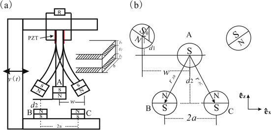
Figure 1. Model of the tri-stable energy harvester. (a) Schematic diagram; (b) geometric diagram of magnets.
Download figure:
Standard image High-resolution imageThe kinetic energy of the cantilever beam can be given by

where L is the length of the whole piezoelectric beam and m is the mass per unit length of the beam. m can be evaluated as ![$m=b{\delta }_{1}{\rho }_{1}+b{\delta }_{2}{\rho }_{2}\left[H\left(s-\frac{L-{L}_{{\rm{p}}}}{2}\right)-H\left(s-\frac{L+{L}_{{\rm{p}}}}{2}\right)\right],$](https://content.cld.iop.org/journals/0964-1726/25/1/015001/revision1/smsaa0857ieqn4.gif) where
where  is the length of the whole piezoelectric layer,
  and
and  are the densities of piezoelectric patches and steel beam respectively, and
  is the width of the substrate and the piezoelectric layer.
  is the Heaviside function to account for the fact that the piezoelectric layer does not cover the entire length of the beams, w denotes the transverse displacement, s is the position coordinate of the beam and y(t) represents the base excitation.
Considering the effect of electromechanical coupling, the potential energy of the whole system is
where  represents the flexural rigidity of the beam and can be given by
where  and
and  denote the Young's modulus of the piezoelectric layer and steel substrate respectively;
  ,
,  and
and  are respectively the distance from the neutral axis to the bottom surface of the substrate, the distance between the neutral axis and the bottom surface of the piezoelectric layer and the distance between the neutral axis and the upper surface of the piezoelectric layer;
  is the electromechanical coupling term;
  is the capacitance of the piezoelectric patches;
  represents the voltage across the piezoelectric layers;
  refers to the potential energy induced by magnet forces.
The virtual work done by non-conservative forces is

where c is the damping coefficient, Q is the electric charge of the piezoelectric layer, and its time rate of change is the electric current passing through the resistive load R, i.e., 
Supposing that the first mode is dominant in the Galerkin expansion of the total selection function, we have

where  is the first mode shape of the beam given by
  and
and  is the generalized displacement of time-dependent mode shapes.
Substituting equation (5) into equations (1), (2) and (4), the kinetic energy, the potential energy and the virtual work will take the following forms:
The rotation angle θ can be approximated in terms of beam elastic displacement as

The displacement perpendicular to  is
is

Since permanent magnets in the structure are all considered as point dipoles (figure 1(b)), according to the geometrical relations, the vectors directed from the fixed magnets (B, C) to the tip magnet (A) are expressed as

where  is the unit vector parallel to
  and
and  is the unit vector perpendicular to
  .
.
The magnetic moment vector  is dependent on the volume of the magnet and given by [13]

where  represents the vector sum of all microscopic magnetic moments for ferromagnetic material and
  is the material volume. The magnetization vector
  is related to the magnet's residual flux density
 where
where  is the magnetic permeability constant.
Based on orthogonal decomposition, the magnetic dipole moment vectors can be written as

The magnetic fields of dipoles B and C acting on dipole A are given by
where  and
and  denote Euclidean norm and vector gradient operator respectively. The potential energy of the magnetic field can be written as
Accordingly the magnetic force can be obtained from

Thus the dynamical coupling equations of the system can be derived from Lagrange equations and written as

where
3. Numerical simulation
According to the parameter values shown in table 1, the stability of the system can be notably affected by the positions of magnets. Figure 2(a) shows the variation of the number of stable equilibrium points with parameters  and a. It should be stressed here that the influences of magnet forces between magnets B, C and A are extremely weak for very large
  in which case the system will exhibit a quasi-linear characteristic. Figure 2(b) shows the variation of potential function with parameter a. At a = 0, i.e., magnets B and C combine to a single magnet, the potential energy shows an obviously bi-stable characteristic. Then as a increases, i.e., the magnets B and C are being separated, the bi-stable potential well turns gradually into a tri-stable one.
Table 1. Structural parameters of the piezoelectric energy harvesting system.
| Description, symbol | Value |
|---|---|
Length of piezoelectric beam, 
|
0.125 m |
Length of piezoelectric layer, 
|
0.015 m |
Width of piezoelectric beam, 
|
0.016 m |
Thickness of piezoelectric layer, 
|
0.0002 m |
Thickness of steel substrate, 
|
0.00 075 m |
Density of piezoelectric layer, 
|
2270 kg m−3 |
Density of steel substrate, 
|
7800 kg m−3 |
Young's modulus of piezoelectric layer, 
|
40 GPa |
Young's modulus of steel substrate, 
|
210 GPa |
Damping coefficient, 
|
20 N s m−1 |
| Coupling coefficient, d31 | −240 × 10−12 C N−1 |
| Electrical permittivity, e33 | 1.2 × 10⁻⁸ F m−1 |
Magnetization vector, (   ) ) |
0.995 × 10⁶ A m−1 |
| Volume of magnet |
 × 0.012 × 0.005 m3 × 0.012 × 0.005 m3 |
Gravitational constant, 
|
9.81 m s−2 |
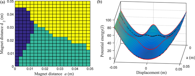
Figure 2. (a) Parameter region: yellow—quasi-linear, green—tri-stable, blue—bi-stable. (b) Potential energy varies with a for d2 = 0.02 m.
Download figure:
Standard image High-resolution imageIn accordance with figure 2(a), by adjusting the magnet distance  or
or  we obtain the potential energy curve of a bi-stable system (a = 0 m, d2 = 0.015 m) and a tri-stable system (a = 0.015 m, d2 = 0.015 m). From the diagram of potential energy (figure 3(a)), it can be seen that the tri-stable system has a lower potential energy barrier than the bi-stable one
  and the distance between the farthest two wells of the tri-stable system is larger than that of bi-stable one, which implies that the jump between the wells occurs more easily and can give rise to a large amplitude of inter-well response. Figure 3(b) shows the restoring forces for linear, quasi-linear, bi-stable and tri-stable systems. Next we will focus on the performance of energy harvesting in the cases of BEH and TEH.
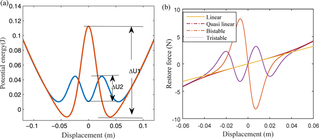
Figure 3. (a) Potential energy function. (b) Restoring force.
Download figure:
Standard image High-resolution image3.1. The case of harmonic excitation
In this part, numerical simulations are carried out to investigate the electrical response of a harvester under base excitation. The governing equations (16) are solved by the Runge–Kutta method. It is assumed that the base excitation is harmonic  where
where  and
and  represent the amplitude and frequency of excitation respectively. The geometric parameters of the harvester are given in table 1.
By varying the frequency of excitation, the two systems will exhibit different characteristics in stability. Figure 4 shows the responses and voltages with frequencies of excitation, while the acceleration is designated as  For figure 4(a), it should be noted that the peaks correspond to the high-energy motion range for BEH and TEH. It is evident that the occurrence frequency of jumps for TEH is lower than that for BEH. For clarity, the phase portraits for BEH and TEH at three excitation frequencies are plotted in figures 4(b)–(d). From the figures, it is apparent that TEH can realize a motion of circulating all equilibrium positions (inter-well motion) and create a large amplitude of response at the low frequency of 10 Hz, whereas BEH is confined in a well and has a response of very small amplitude. As the excitation frequency increases to 20 Hz, both BEH and TEH can realize regular jumps between potential wells. Then as the frequency further increases to 30 Hz, both responses are restricted in a single potential well, which hinders the occurrence of large responses and high output voltages.

Figure 4. (a) RMS voltage for BEH and TEH. (b) Phase portrait for 10 Hz. (c) Phase portrait for 20 Hz. (d) Phase portrait for 30 Hz.
Download figure:
Standard image High-resolution image3.2. The case of stochastic excitation
To investigate the harvesting efficiency under stochastic excitation, we designate the excitation as a Gaussian white noise process  whose mean and correlation function are given as

where  denotes the expected value and
  is the noise intensity.
The performance of the piezo-magnetoelastic structure can be represented by the RMS output voltage and the efficiency of power conversion, which is defined by

where  and
and  are the effective values of electrical and mechanical power respectively. For an instantaneous power, its effective value is defined as

where  represents the instantaneous power at time t. For this system, its instantaneous electric power harvested is defined as
  where
where  is the current and R the resistance; its mechanical counterpart is defined as
  [30]. In addition to generating electrical power, mechanical energy is also transformed to kinetic energy, potential energy and is dissipated by damping.
Numerical simulations are carried out with the system parameters listed in table 1. The Euler–Maruyama and Monte Carlo methods are applied in the stochastic simulation [28, 31]. In order to obtain the relation between the output power and the distance between magnets, we calculate the output power at different distances for TEH and BEH. Let d2T denote the distance between the magnets A and BC in TEH, and d2B denote that in BEH. The corresponding simulation results at excitation intensity  are shown in figure 5. It can be seen that there appears a peak for output power in both TEH and BEH. Thus it can be concluded that in both BEH and TEH, there is an optimal distance between magnets at which the system can produce the largest output power. And as shown in figure 5, the peak for BEH appears at
  (figure 5(a)), while that for TEH appears at
  (figure 5(b)).

Figure 5. The influence of the distance between magnets A and BC on output power. (a) BEH; (b) TEH.
Download figure:
Standard image High-resolution imageFigures 6 and 7 show the responses and outputs of the BEH and TEH as the excitation intensity  increases. Figure 6 shows the signal-to-noise ratio (SNR =
  [28], where
  and
and  are the standard deviations of response and excitation) and RMS voltage. It should be noted that the pronounced peaks imply the occurrence of coherence resonance, in which the system possesses a nearly regular jump between the potential wells. As shown in figure 6(a), the peak for the tri-stable state appears at
  while that for the bi-stable state appears at
  This indicates that the tri-stable state can lead the system to coherence resonance at a lower noise intensity. Then according to figure 6(b), it is evident that the tri-stable harvester has the higher voltage of harvesting.

Figure 6. (a) Signal-to-noise ratio and (b) RMS output voltage.
Download figure:
Standard image High-resolution image
Figure 7. (a) Output power and (b) energy conversion efficiency.
Download figure:
Standard image High-resolution imageFigure 7 illustrates the energy conversion efficiency and power output versus  for BEH and TEH. It proves that the TEH can give out the larger output power and achieve the higher energy conversion efficiency.
Figures 8 and 9 show the time histories of displacements of the beam tip and the output voltages simultaneously produced by the piezoelectric patches at  and
and  respectively. From the results, it can be seen that the jump between potential wells occurs at
  for TEH, whereas for BEH the response is still restricted in a single well (figure 8). The highest voltage for TEH can reach Vmax = 13.2 V, while that for BEH is only Vmax = 2.3 V.
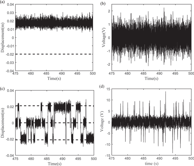
Figure 8. Response of the energy harvesting system and provided voltage for  (a, b) BEH. (c, d) TEH.
Download figure:
Standard image High-resolution image
Figure 9. Response of the energy harvesting system and provided voltage for  (a, b) BEH. (c, d) TEH.
Download figure:
Standard image High-resolution imageThen as  increase to 0.1, BEH and TEH both undergo a jump between potential wells, or coherence resonance. Since BEH has two close potential wells and a high potential barrier, the jump does not happen frequently and the output voltage is relatively small. For TEH, on the other hand, there exist three potential wells and the potential barriers are relatively lower, which leads to jumping between three potential wells more frequently and produces a large amplitude of response, hence giving out a high output voltage. This can be seen clearly from the RMS output voltages for the two states (
 for TEH and
  for BEH) (figure 9).
4. Experimental validation
To validate the results of the analysis for BEH and TEH, corresponding experiments are designed and carried out. Figure 10 shows the experimental equipment including bi-stable and tri-stable energy harvesters used for verification. The shaker produces the excitation, which actuates the ferromagnetic beam that has piezoelectric PZT patches. The beam is made of stainless steel with dimensions of  The PZT patches have dimensions of
  All permanent magnets are NdFeB cylinder magnets. All magnets have an identical diameter of
  and thickness of
  .
.

Figure 10. Experimental setup. (a) Bi-stable energy harvester (
 ) and (b) tri-stable energy harvester (
 = 15 mm).
Download figure:
Standard image High-resolution imageIn experiments, the stochastic excitation is chosen for the shaker and its power spectral density  is varied from 0.004 to 0.03 g2 Hz–1 for BEH and TEH. Figure 10(a) shows the standard deviation of dynamic strain versus that of excitation intensity. It can be observed that there appears a peak value for both BEH and TEH, which corresponds to the coherence resonance phenomenon. The experimental results are shown in figures 11–13. For figure 11(a), it is evident that the curve of
  has the nearly same trend as that of the SNR simulation results shown in figure 6. Figure 11(b) presents the open-circuit RMS voltages of BEH and TEH for different intensities of excitation. The experimental results are consistent with the trend obtained from the simulations (refer to figure 6(b)). From figures 11(a) and (b) we can conclude that, compared to BEH, the threshold for coherence resonance to occur in TEH can be moved lower to D = 0.008 g2 Hz–1, which implies that the much lower intensity of excitation can induce the coherence resonance. Therefore the effective range of intensity for TEH is much wider than that for BEH for the broadband stochastic excitation.

Figure 11. (a) Experimental standard deviation of dynamic strain versus excitation intensity and (b) experimental RMS open-circuit voltages for BEH and TEH.
Download figure:
Standard image High-resolution image
Figure 12. The system's dynamic strains and voltages at  g2 Hz–1. (a, b) BEH. (c, d) TEH.
Download figure:
Standard image High-resolution image
Figure 13. The dynamic strains at  g2 Hz–1. (a, b) BEH. (c, d) TEH.
Download figure:
Standard image High-resolution image
Figures 12 and 13 show the time histories of the strains and corresponding open-circuit voltages for D = 0.004 and D = 0.03 g2 Hz–1. When the intensity of the stochastic excitation is fairly low, the jump in response cannot happen in BEH (figure 12(a)), where the tip displacement is trapped in a single well. But the jump starts to occur in TEH (figure 12(c)), and the output voltage reaches a high value. When the excitation becomes large (figure 13), the strain responses clearly illustrate that both systems tend to the large-amplitude oscillation originating from the jump between potential wells (figures 13(a) and (c)), and the harvesting voltages both rise. But in TEH the response jumps frequently and produces a dense high voltage (figures 13(b) and (d)).
5. Conclusions
This paper proposes a piezoelectric energy harvester with tri-stable potential wells induced by external magnetic fields. The coupling equations for the system are derived and solved. Parameter regions and the expression for the restoring force for BEH and TEH in terms of the distance between magnets are given. Numerical simulations and experimental validation are carried out to compare and analyze the efficiencies of BEH and TEH for stochastic excitation. From the results, following conclusions can be drawn.
- 1.With increasing distance between magnets, the system proposed can transform from two potential wells to three potential wells. The barriers between the three potential wells are lower, hence inter-well oscillation can occur more easily in the TEH, and the corresponding amplitude is larger than that of BEH. In the case of harmonic excitation, TEH has the lower frequency threshold for jumping between potential wells, or a high-energy solution.
- 2.In the case of stochastic excitation, TEH begins jumping between wells at a low excitation intensity. Thereafter, with increasing excitation intensity, TEH will reach a state of frequent jumping between three potential wells and give out a dense high voltage. The energy conversion rate and RMS voltage indicate that the energy harvesting efficiency of TEH outperforms that of BEH due to this coherence resonance.
- 3.For both BEH and TEH, experiments are carried out to validate their theoretical analysis. The experimental results are in good agreement with those of simulation and confirm that TEH is more efficient in harvesting than BEH.
- 4.The performance of the TEH depends on its geometric parameters. Improper parameters will make the middle potential well deeper, which will restrict the response and cannot lead to the occurrence of inter-well motion at low stochastic excitation.
Acknowledgments
This work is supported by the Natural Science Foundation of China (Grant No. 11172234).