
Abstract
A comprehensive statistical analysis is performed for structural health monitoring (SHM). The analysis starts by obtaining the baseline principal component analysis (PCA) model and projections using measurements from the healthy or undamaged structure. PCA is used in this framework as a way to compress and extract information from the sensor-data stored for the structure which summarizes most of the variance in a few (new) variables into the baseline model space. When the structure needs to be inspected, new experiments are performed and they are projected into the baseline PCA model. Each experiment is considered as a random process and, consequently, each projection into the PCA model is treated as a random variable. Then, using a random sample of a limited number of experiments on the healthy structure, it can be inferred using the χ2 test that the population or baseline projection is normally distributed with mean μh and standard deviation σh. The objective is then to analyse whether the distribution of samples that come from the current structure (healthy or not) is related to the healthy one. More precisely, a test for the equality of population means is performed with a random sample, that is, the equality of the sample mean μs and the population mean μh is tested. The results of the test can determine that the hypothesis is rejected (μh ≠ μc and the structure is damaged) or that there is no evidence to suggest that the two means are different, so the structure can be considered as healthy. The results indicate that the test is able to accurately classify random samples as healthy or not.
Export citation and abstract BibTeX RIS
1. Introduction
Among all the elements that are integrated into a structural health monitoring (SHM) system, methods or strategies for damage detection are nowadays playing a key role in improving the operational reliability of critical structures in several industrial sectors [3]. The essential paradigm is that a self-diagnosis and some level of detection and classification of damage are possible through the comparison of the in-service dynamic time responses of a structure with respect to baseline reference responses recorded in ideal healthy operating conditions [5]. These dynamic time responses recorded in each test, even in stable environmental and operational conditions, present the main characteristic that they are not repeatable. This means that always exists variation between measurements. Such variability may be caused by random measurement errors: measurement instruments are often not perfectly calibrated and thus generate discordant interpretation and reporting of the results.
Since the dynamic response of a structure can be considered as a random variable, a set of dynamic responses gathered from several experiments can be defined as a sample variable, and all possible values of the dynamic response as the population variable. Therefore, the process of drawing conclusions about the state of the structure from several experiments by using statistical methods is usually called statistical inference for damage diagnosis. In the SHM field, statistical inference can be considered as one of the emerging technologies that will have an impact on the damage prognosis process [4, 2].
In general, there are two kinds of statistical inference: (i) estimation, which uses sample variables to predict an unknown parameter of the population variable, and (ii) hypothesis testing, which uses sample variables to determine whether a parameter fulfils a specific condition and to test a hypothesis about a population variable. In this last context, a classical hypothesis test is used to compare extracted statistical quantities from statistical time series models like mean, normalized autocovariance function, cross covariance function, power spectral density, cross spectral density, frequency response function, squared coherence, residual variance, likelihood function, residual sequences, among others [7]. A hypothesis testing technique called a sequential probability ratio test (SPRT) has been combined with time series analysis and neural networks for damage classification in [14]. The usefulness of the proposed approach is demonstrated using a numerical example of a computer hard disk and an experimental study of an eight degree-of-freedom spring–mass system. Afterwards, the performance of the SPRT is improved by integrating extreme value statistics, which specifically models the behaviour in the tails of the distribution of interest into the SPRT. A model of a three-storey building was constructed in a laboratory environment to assess the approach [12]. Recently, a generalized likelihood ratio test (GLRT) was used to compare the fit of minimum mean square error (MMSE) model parameters in order to detect damage in a scaled wooden model bridge [8, 9].
In previous work, the authors have been investigating novel multi-actuator piezoelectric systems for detection and localization of damage. These approaches combine (i) the dynamic response of the structure at different exciting and receiving points, (ii) the correlation of dynamical responses when some damage appears in the structure by using principal component analysis (PCA) and statistical measures that are used as damage indices and (iii) the contribution of each sensor to the indices, which is used to localize the damage [10, 11]. For detection, damage indices are calculated by analysing the variability of the measured data stored in a matrix X and a new projected matrix T calculated as T = XP, where P is a proper linear transformation as detailed in section 2.2.
Following the same framework and considering dynamic responses as random variables, this paper is focused on the development of a damage detection indicator that combines a data driven baseline model (reference pattern obtained from the healthy structure) based on principal component analysis (PCA) and hypothesis testing. As said before, the use of hypothesis testing is not new in this field. The novelty of this work is based on (i) the nature of the data used in the test since we are using scores instead of the measured response of the structure [7] or the coefficients of an autoregressive model [17], (ii) the number of data used since our test is based on two random samples instead of two characteristic quantities [6]. The proposed development starts by obtaining the baseline PCA model and the subsequent projections using the healthy structure. When the structure needs to be inspected, new experiments are performed and they are projected onto the baseline PCA model. Each experiment is considered as a random process and the projection onto each principal component is a random variable. The objective is to analyse whether the distribution of the variable associated with the current structure is related to the healthy one.
This paper is organized as follows. Section 2 describes how the baseline model is built using PCA including the experimental set-up used to validate the proposed approach. In section 3 the damage detection based on hypothesis testing is developed. In particular, a study of normality of the distribution is first performed. Secondly, a hypothesis test is formulated yielding the structural damage indicator. Section 4 presents the experimental results, showing an acceptable level of sensitivity, specificity and reliability for the test. Finally, some conclusions are drawn.
2. Data driven baseline modelling based on PCA
In this paper a specific experimental set-up based on the analysis of changes in the vibrational properties is used as an illustrative example in order to explain, validate and test the proposed methodology. However, this methodology can be applied to any more general structure.
2.1. Experimental set-up
The small aluminum plate (25 cm × 25 cm × 0.2 cm) in figure 1 (top) is used to experimentally validate the proposed approach in this work. The plate is suspended by two elastic ropes in a metallic frame in order to isolate the environmental noise and remove boundary conditions (figure 2). Four piezoelectric transducer discs (PZTs) are attached to the surface. Each PZT is able to produce a mechanical vibration (Lamb waves in a thin plate) if some electrical excitation is applied (actuator mode). Besides, the PZTs are able to detect time varying mechanical response data (sensor mode). In each phase of the experimental stage, just one PZT is used as the actuator (exciting the plate) and the rest are used as sensors (and thus record the dynamical response). A total of 100 experiments were performed using the healthy structure: 50 for the baseline (BL) and 50 for testing (Un, which stands for undamaged, is an abbreviation used throughout the paper). Additionally, nine damaged areas (D1, D2 ...D9) were simulated by adding different masses at different locations. For each damaged area, 50 experiments were implemented, resulting in a total of 450 experiments. The excitation was a sinusoidal signal of 112 kHz modulated by a Hamming window (see figure 3 (top)). An example of the signal collected by PZT2 is shown in figure 3 (bottom).
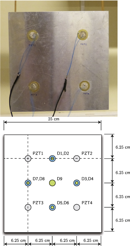
Figure 1. Aluminum plate (top). Dimensions and piezoelectric transducer locations (bottom).
Download figure:
Standard image High-resolution image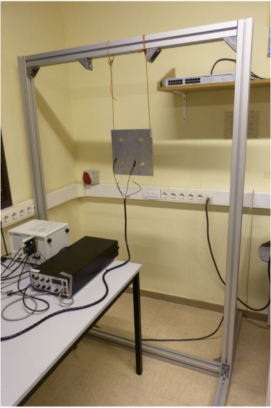
Figure 2. The plate is suspended by two elastic ropes in a metallic frame.
Download figure:
Standard image High-resolution image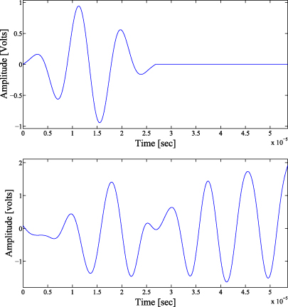
Figure 3. Excitation signal (top) and dynamic response recorded by PZT2 (bottom).
Download figure:
Standard image High-resolution image2.2. Principal component analysis (PCA): theoretical background
Let us address the analysis of a physical process by measuring several variables (sensors) at a number of time instants. In this paper, the collected data are arranged as follows:
This n × (N⋅L) matrix contains information from N sensors at L discretization instants and n experimental trials. In this way, each row vector represents, for a specific experimental trial, the measurements from all the sensors at every specific time instant. In the same way, each column vector represents measurements from one sensor at one specific time instant in the whole set of experiment trials.
The goal of principal component analysis (PCA) is to discern which dynamics are more important in the system, which are redundant and which are just noise [10]. This goal is essentially achieved by determining a new space (coordinates) to re-express the original data filtering noise and redundancies based on the variance–covariance structure of the original data. In other words, the goal is to find an (N⋅L) × (N⋅L) linear transformation orthogonal matrix P, which is used to transform the original data matrix X into the form

where  n×(N⋅L)(
 ) is the vector space of n × (N⋅L) matrices over , P can be called the principal components of the data set (or loading matrix in other articles) and T the projected or transformed matrix to the principal component space (or score matrix in other articles). In the full dimensional case (using all the (N⋅L) principal components), this projection is invertible (since the orthogonality of P implies PPT = I) and the original data can be recovered as X = TPT.
The matrix P can be determined by means of the singular value decomposition (SVD) of the covariance matrix (see equation (3)). The subspaces in PCA are defined by the eigenvectors and eigenvalues of the covariance matrix as follows:


where the eigenvectors of CX are the columns of P, and the eigenvalues are the diagonal terms of Λ (the off-diagonal terms are zero). The eigenvectors pj, j = 1,...,N⋅L forming the transformation matrix P (its columns) are sorted according to the eigenvalues by descending order and they are called the principal components of the data set. The eigenvector with the highest eigenvalue represents the most important pattern in the data with the largest quantity of information.
However, PCA also seeks to reduce the dimensionality of the data set X by choosing only a reduced number r of principal components (r < N⋅L), that is, just a few eigenvectors associated with the highest eigenvalues. Now, with  given by the reduced matrix
  as
as  , it is not possible to fully recover X, but
  can be projected back onto the original (N⋅L)-dimensional space to obtain another data matrix as follows:

Therefore, the difference between the original data matrix X and the back-projected data  is defined as the residual error matrix E as follows:

or, equivalently,

The residual error matrix represents the variability not described by the projected back data  .
.
Although the real measures obtained from the sensors (matrix X) as a function of time represent physical magnitudes, when these measures are projected (matrix T) and the scores are obtained, these scores are dimensionless and no longer represent physical magnitudes. The key aspect in this approach is that the scores from different experiments can be compared with the reference pattern to try to detect a different behaviour.
2.3. PCA modelling
Let us consider the structure in a fully healthy state where we perform a set of experiments as explained in section 2.1. For each actuator phase (PZT1 as actuator, PZT2 as actuator, and so on) and using the signals recorded by the sensors, the matrix Xh is defined and organized as in equation (1) and scaled as explained in [10]. PCA modelling essentially consists of calculating the projection matrix P for each phase (equation (2)), which offers a better and dimensionally reduced representation of the original data Xh. Matrix P, renamed Pmodel, will be considered as the model of the undamaged structure to be used in the health diagnosis, as illustrated in figure 4.
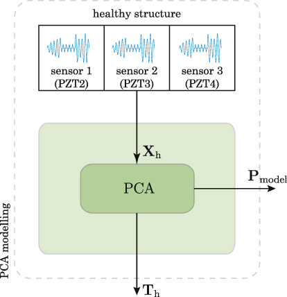
Figure 4. A PCA model Pmodel is built for each actuator phase using the signals Xh recorded by the sensors during the experiments with the undamaged structure.
Download figure:
Standard image High-resolution image3. Damage detection based on hypothesis testing
The current structure to diagnose is subjected to a predefined number of experiments and a new data matrix Xc is constructed with the measured data. The number of experiments can be as many as wanted, but the number of sensors and collected samples (data-points) must be the same as was used in the modelling stage; that is, the number of columns of Xc must agree with that of Xh. This matrix Xc is projected onto the baseline PCA model, as detailed in section 3.1. Projections onto the first components (scores) are obtained and used for the construction of the simple random samples to be compared and finally to obtain the damage indicator (see figure 5).

Figure 5. The structure to be diagnosed is subjected to a predefined number of experiments and a data matrix Xc is constructed. This matrix is projected onto the baseline PCA model Pmodel to obtain the projections onto the first components Tc.
Download figure:
Standard image High-resolution image3.1. Random variables and random samples
Let us start this section by first defining what we consider a random variable. Assume that for a particular actuator phase (for instance, PZTi as actuator, i = 1,2,3,4) we have built the baseline PCA model (matrix  ) using the signals recorded by the sensors in a fully healthy state as in sections 2.2 and 2.3. Assume also that we further perform an experiment as described in section 2.1. The time responses measured by the sensors are discretized and arranged in a row vector ri of dimension N⋅L, where N is the number of sensors and L is the number of discretization instants. The numbers of sensors and number discretization instants must coincide with those that were used when constructing
  . The columns of
  are the principal components. In turn, the size of each column is N⋅L. Choosing the jth principal component (j = 1,...,n),
  , the projection of the measured data onto this principal component is the inner product (see equation (2))

Since the dynamic response of a structure can be considered as a random process, the measurements in ri are also random. Therefore,  inherits this nature and it will be considered as a random variable to construct the statistical approach in this work.
By repeating this experiment several times and using equation (8) we have a random sample of the variable  which can be considered as a baseline. When the structure has to be diagnosed, new experiments should be performed to obtain a random sample, which will be compared with the baseline sample. As an illustrative example, in figure 6 two samples are represented; one is the baseline sample (top) and the other corresponds to damage 3 (bottom). This example corresponds to actuator phase 1 and the first principal component, so that figure 6 plots the values of the random variable
  . The baseline sample is made by 50 experiments and the diagnosis sample consists of 10 experiments.

Figure 6. Baseline sample (top) and sample from the structure to be diagnosed (bottom).
Download figure:
Standard image High-resolution image3.2. Detection phase
The main idea in statistical inference is to obtain conclusions or make generalizations about the population from sampled information. For the generalizations to be valid, the sample must meet certain requirements. In this work, the framework of statistical inference is used with the objective of the classification of structures as healthy or damaged. With this goal, a chi-square goodness-of-fit test is first performed to test the hypothesis that the samples are normally distributed [13]. A test for the equality of means is then performed when sampling from independent normal distributions with variances that are unknown and not necessarily equal.
3.2.1. The chi-square goodness-of-fit test
In figure 7, the results of the chi-square goodness-of-fit test applied to the samples described in section 2.1 are depicted. It can be seen by observing the upper-left barplot diagram that all the samples are normally distributed except for those corresponding to the damaged areas D2 and D7. More precisely, their p-values are smaller than the level of significance (horizontal red dashed line), thus rejecting the hypothesis of normality in these two samples. In the rest of the diagrams, one can see both (a) the estimation of the mean and standard deviation of each sample and (b) the superposition of the density function of the normal distribution and the corresponding sampling distribution.
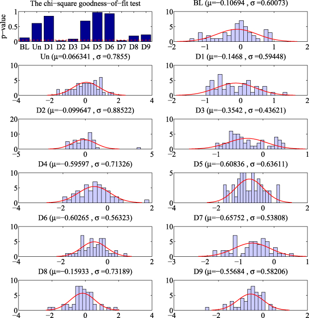
Figure 7. Results of the chi-square goodness-of-fit test applied to the samples described in section 2.1. 'BL' stands for baseline projection, 'Un' for the sample obtained from the undamaged structure and 'Di' for damaged area number i, where i = 1,2,...,9. It can be shown by observing the upper-left barplot diagram that all the samples are normally distributed except those corresponding to the damaged areas D2 and D7 (see section 3.2.1).
Download figure:
Standard image High-resolution image3.2.2. Test for the equality of means
The objective of this work is to examine whether the distribution of the samples that are obtained from the current structure (healthy or not) is related to the distribution of the baseline. To achieve this end, a test for the equality of means will be performed. Let us consider that (a) the baseline projection is a random sample of a random variable having a normal distribution with unknown mean μh and unknown standard deviation σh and (b) the random sample of the current structure is also normally distributed with unknown mean μc and unknown standard deviation σc. Let us finally consider that the variances of these two samples are not necessarily equal, as can be observed in figure 7. As said before, the idea is to test whether these means are equal, that is, μh = μc, or equivalently μh − μc = 0. Therefore, the statistical hypothesis test used is


that is, the null hypothesis is 'the two means are equal' and the alternative hypothesis is 'the two means are different'. Roughly speaking, if the result of the test is that the null hypothesis is rejected, this would indicate the existence of some damage in the structure. Otherwise, if the null hypothesis is not rejected, the current structure is classified as healthy.
The test is performed based on the Welch–Satterthwaite method [15], which is outlined below. When random samples of size nh and nc, respectively, are taken from two normal distributions N(μh,σh) and N(μc,σc) and the population variances are unknown, the random variable
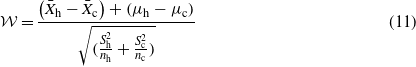
can be approximated with a t-distribution with ν degrees of freedom; that is,

where
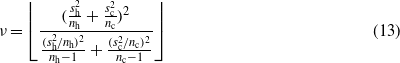
and where  is the sample mean as a random variable; S2 is the sample variance as a random variable; s2 is the variance of a sample; ⌊⋅⌋ is the floor function.
The value of the standardized test statistic using this method is defined as
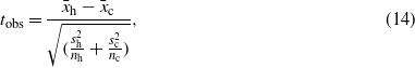
where  is the mean of a particular sample. This quantity tobs is the damage indicator. We can then construct the following test:


where t⋆ is such that

and α is the chosen risk (significance) level for the test. More precisely, the null hypothesis is rejected if |tobs| > t⋆ (this would indicate the existence of some damage in the structure). Otherwise, if |tobs| ≤ t⋆ there is no statistical evidence to suggest that both samples are normally distributed but with different means, thus indicating that no damage in the structure has been found. This idea is represented in figure 8.
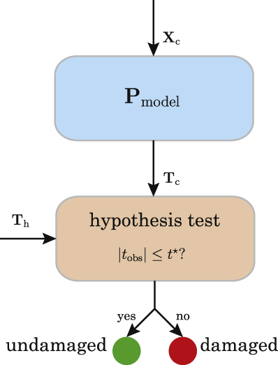
Figure 8. Damage detection will be based on testing for significant changes in the distributions of samples Th and Tc.
Download figure:
Standard image High-resolution image4. Experimental results
4.1. Type I and Type II errors
As said in section 2.1, the experiments are performed in four independent phases: (i) piezoelectric transducer 1 (PZT1) is configured as the actuator and the rest of the PZTs as sensors, (ii) PZT2 as the actuator, (iii) PZT3 as the actuator and (iv) PZT4 as the actuator. In order to analyse the influence of each projection into the PCA model (score), the results of the first three scores have been considered. In this way, a total of 12 scenarios were examined. For each scenario, a total of 50 samples of ten experiments each (five for the undamaged structure and five for the damaged structure with respect to each of the nine different types of damage) plus the baseline are used to test for the equality of means, with a level of significance α = 0.30 (the choice of this level of significance will be justified in section 4.2). Each set of 50 testing samples is categorized as follows: (i) number of samples from the healthy structure (undamaged sample) which were classified by the hypothesis test as 'healthy' (fail to reject H0); (ii) undamaged sample classified by the test as 'damaged' (reject H0); (iii) samples from the damaged structure (damaged sample) classified as 'healthy'; and (iv) damaged sample classified as 'damaged'. The results for the 12 different scenarios presented in table 2 are organized according to the scheme in table 1. It can be stressed that for each scenario in table 2 the sum of the columns is constant: five samples in the first column (undamaged structure) and 45 samples in the second column (damaged structure).
Table 1. Scheme for the presentation of the results in table 2.
| Undamaged sample (H0) | Damaged sample (H1) | |
|---|---|---|
| Fail to reject H0 | Correct decision | Type II error (missing fault) |
| Reject H0 | Type I error (false alarm) | Correct decision |
Table 2. Categorization of the samples with respect to the presence or absence of damage and the result of the test for each of the four phases and the three scores.
| PZT1 act. | PZT2 act. | PZT3 act. | PZT4 act. | ||||||||
|---|---|---|---|---|---|---|---|---|---|---|---|
| H0 | H1 | H0 | H1 | H0 | H1 | H0 | H1 | ||||
| Score 1 | |||||||||||
| Fail to reject H0 | 4 | 15 | 3 | 0 | 2 | 4 | 3 | 23 | |||
| Reject H0 | 1 | 30 | 2 | 45 | 3 | 41 | 2 | 22 | |||
| Score 2 | |||||||||||
| Fail to reject H0 | 4 | 0 | 1 | 4 | 4 | 5 | 5 | 7 | |||
| Reject H0 | 1 | 45 | 4 | 41 | 1 | 40 | 0 | 38 | |||
| Score 3 | |||||||||||
| Fail to reject H0 | 4 | 2 | 4 | 1 | 4 | 6 | 3 | 6 | |||
| Reject H0 | 1 | 43 | 1 | 44 | 1 | 39 | 2 | 39 | |||
In this table, it is worth noting that two kinds of misclassification are presented which are denoted as follows.
- (i)Type I error (or false positive), when the structure is healthy but the null hypothesis is rejected and therefore it is classified as damaged. The probability of committing a type I error is α, the level of significance.
- (ii)Type II error (or false negative), when the structure is damaged but the null hypothesis is not rejected and therefore it is classified as healthy. The probability of committing a type II error is called β.
4.2. Sensitivity and specificity
Two statistical measures can be employed here to study the performance of the test: the sensitivity and the specificity. The sensitivity, also called as the power of the test, is defined, in the context of this work, as the proportion of samples from the damaged structure which are correctly identified as such. Thus, the sensitivity can be computed as 1 − β. The specificity of the test is defined, also in this context, as the proportion of samples from the undamaged structure that are correctly identified, and can be expressed as 1 − α.
The sensitivity and specificity of the test with respect to the 50 samples in each scenario have been included in table 4. For each scenario in this table, the results are organized as shown in table 3.
Table 3. Relationship between type I and type II errors.
| Undamaged sample (H0) | Damaged sample (H1) | |
|---|---|---|
| Fail to reject H0 | Specificity (1 − α) | False negative rate (β) |
| Reject H0 | False positive rate (α) | Sensitivity (1 − β) |
Table 4. Sensitivity and specificity of the test for each scenario.
| PZT1 act. | PZT2 act. | PZT3 act. | PZT4 act. | ||||||||
|---|---|---|---|---|---|---|---|---|---|---|---|
| H0 | H1 | H0 | H1 | H0 | H1 | H0 | H1 | ||||
| Score 1 | |||||||||||
| Fail to reject H0 | 0.80 | 0.33 | 0.60 | 0.00 | 0.40 | 0.09 | 0.60 | 0.51 | |||
| Reject H0 | 0.20 | 0.67 | 0.40 | 1.00 | 0.60 | 0.91 | 0.40 | 0.49 | |||
| Score 2 | |||||||||||
| Fail to reject H0 | 0.80 | 0.00 | 0.20 | 0.09 | 0.80 | 0.11 | 1.00 | 0.16 | |||
| Reject H0 | 0.20 | 1.00 | 0.80 | 0.91 | 0.20 | 0.89 | 0.00 | 0.84 | |||
| Score 3 | |||||||||||
| Fail to reject H0 | 0.80 | 0.04 | 0.80 | 0.02 | 0.80 | 0.13 | 0.60 | 0.13 | |||
| Reject H0 | 0.20 | 0.96 | 0.20 | 0.98 | 0.20 | 0.87 | 0.40 | 0.87 | |||
It is worth noting that type I errors are frequently considered to be more serious than type II errors. However, in this application a type II error is related to a missing fault whereas a type I error is related to a false alarm. In consequence, type II errors should be minimized. Therefore, a small level of significance of 1%, 5% or even 10% would lead to a reduced number of false alarms but a higher rate of missing faults. This is the reason for the choice of a level of significance of 30% in the hypothesis test.
The results show that the sensitivity of the 1 − β test is close to 100%, as desired, with an average value of 86.58%. The sensitivity with respect to the projection onto the second and third components (second and third scores) is increased, on average, to 91.50%. The average value of the specificity is 68.33%, which is very close to the expected value of 1 − α = 70%.
4.3. Reliability of the results
The results in table 6 are computed using the scheme in table 5. This table is based on the Bayes theorem [1], where P(H1|accept H0) is the proportion of samples from the damaged structure that have been incorrectly classified as healthy (true rate of false negatives) and P(H0|acceptH1) is the proportion of samples from the undamaged structure that have been incorrectly classified as damaged (true rate of false positives).
Table 5. Relationship between the proportion of false negatives and false positives.
| Undamaged sample (H0) | Damaged sample (H1) | |
|---|---|---|
| Fail to reject H0 | P(H0|acceptH0) | True rate of false negatives P(H1|acceptH0) |
| Reject H0 | True rate of false positives P(H0|acceptH1) | P(H1|acceptH1) |
Since these two true rates are not functions of the accuracy of the test alone, but also functions of the actual rate or frequency of occurrence within the test population, some of the results are not as good as desired. The results in table 6 can be improved without affecting the results in table 4 by considering an equal number of samples from the healthy structure and from the damaged structure.
Table 6. True rate of false positives and false negatives.
| PZT1 act. | PZT2 act. | PZT3 act. | PZT4 act. | ||||||||
|---|---|---|---|---|---|---|---|---|---|---|---|
| H0 | H1 | H0 | H1 | H0 | H1 | H0 | H1 | ||||
| Score 1 | |||||||||||
| Fail to reject H0 | 0.21 | 0.79 | 1.00 | 0.00 | 0.33 | 0.67 | 0.12 | 0.88 | |||
| Reject H0 | 0.03 | 0.97 | 0.04 | 0.96 | 0.07 | 0.93 | 0.08 | 0.92 | |||
| Score 2 | |||||||||||
| Fail to reject H0 | 1.00 | 0.00 | 0.20 | 0.80 | 0.44 | 0.56 | 0.42 | 0.58 | |||
| Reject H0 | 0.02 | 0.98 | 0.09 | 0.91 | 0.02 | 0.98 | 0.00 | 1.00 | |||
| Score 3 | |||||||||||
| Fail to reject H0 | 0.67 | 0.33 | 0.80 | 0.20 | 0.40 | 0.60 | 0.33 | 0.67 | |||
| Reject H0 | 0.02 | 0.98 | 0.02 | 0.98 | 0.03 | 0.97 | 0.05 | 0.95 | |||
4.4. The receiver operating curves
An additional study has been developed based on the receiver operating curves (ROCs) to determine the overall accuracy of the proposed method. These curves represent the trade-off between the false positive rate and the sensitivity in table 3 for different values of the level of significance that is used in the statistical hypothesis testing. Note that the false positive rate is defined as the complement of the specificity, and therefore these curves can also be used to visualize the close relationship between specificity and sensitivity. It can also be remarked that the sensitivity is also called the true positive rate or probability of detection [16]. More precisely, for each scenario and for a given level of significance the pair of numbers

is plotted. We have considered 49 levels of significance within the range [0.2,0.98] and with a difference of 0.02. Therefore, for each scenario 49 connected points are depicted, as can be seen in figure 9.
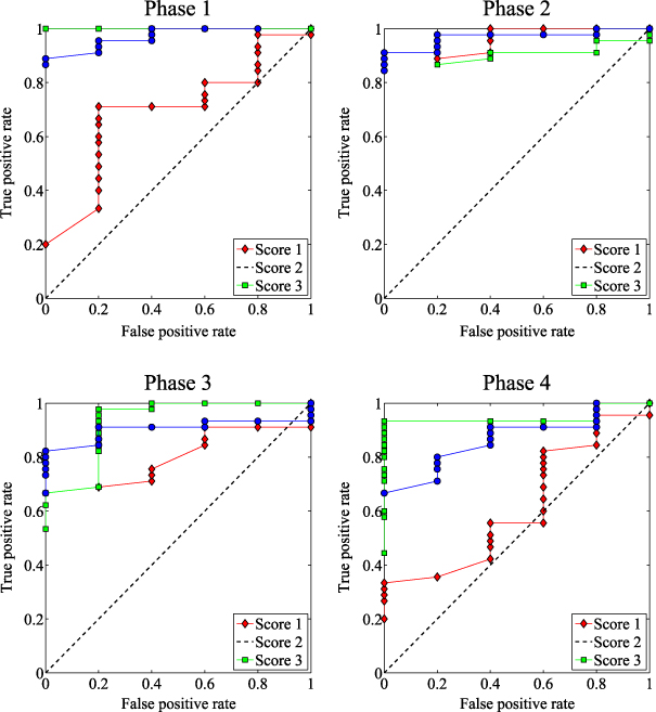
Figure 9. The ROCs for the three scores for each phase.
Download figure:
Standard image High-resolution imageThe placement of these points can be interpreted as follows. Since we are interested in minimizing the number of false positives while maximizing the number of true positives, these points must be placed in the upper-left corner as much as possible. However, this is impossible because there is also a relationship between the level of significance and the false positive rate. Therefore, a method can be considered acceptable if these points lie within the upper-left half-plane.
As said before, the ROCs for all possible scenarios are depicted in figure 9. On one hand, in phase 1 (PZT1 as actuator) and phase 4 (PZT4 as actuator), the first score (diamonds) presents the worst performance because some points are very close to the diagonal or even below it. However, in the same phases, the second and third scores present better results. It may be surprising that the results related to the first score are not as good as those related to the rest of the scores, but in section 4.5 this will be justified. On the other hand, all scores in phases 2 and 3 present very good performance in damage detection.
The curves are similar to stepped functions because we have considered five samples from the undamaged structure and therefore the possible values for the false positive rate (the values on the x-axis) are 0, 0.2, 0.4, 0.6, 0.8 and 1. Finally, we can say that the ROCs provide a statistical assessment of the efficacy of a method and can be used to visualize and compare the performance of multiple scenarios.
4.5. Analysis and discussion
Although the first score has the highest proportion of variance, it is not possible to visually separate between the baseline and the test. Each of the subfigures in figure 10 shows the comparison between the first scores of the baseline experiments and the test experiments for each damaged area. A similar comparison can be found in figure 11, where all the observation points (first score of each experiment) are depicted in a single chart. The rest of the scores do not allow a visual grouping.
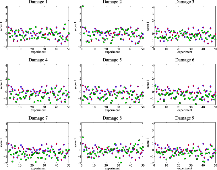
Figure 10. First scores for baseline experiments (diamonds) and testing experiments (circles).
Download figure:
Standard image High-resolution image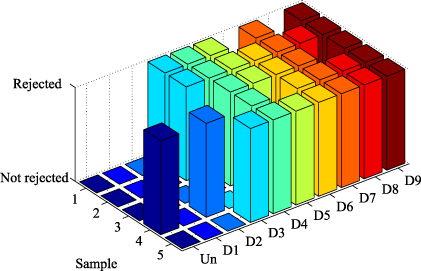
Figure 11. Results of the hypothesis test considering the first score and PZT1 as the actuator.
Download figure:
Standard image High-resolution image
One of the scenarios with the worst results is the one that considers PZT1 as the actuator and the first score, because the false negative rate is 33%, the false positive rate is 20% and the true rate of false negatives is 79% (see tables 4 and 6). These results, which are extracted from table 2, are illustrated for each state of the structure separately in figure 11. Just one of the five samples of the healthy structure has been wrongly rejected (false alarm), whereas all the samples of the structure with damage D1 have been wrongly not rejected (missing fault). Only one of the five samples of the structure with damage D2 has been correctly rejected (correct decision). In this case, however, the bad result could be due to the lack of normality (figure 7). This lack of normality leads to results that cannot be reliable. In fact, these samples should not have been used for a hypothesis test. The samples of the structure with damage D7 are not normally distributed, although in this case the results are correct. This problem can be solved by repeating the test excluding experiments with these damaged areas (D2 and D7) or eliminating the outliers.
Contrary to what may seem reasonable, the projection on the first component (which represents the largest variance of the original data) is not always the best option to detect and distinguish damage. This fact can be explained because the PCA model is built using the data from the healthy structure and, therefore, the first component captures the maximal variance of these data. However, when new data are projected into this model, there is no longer a guarantee of the existence of maximal variance in these new data.
5. Conclusions
In real life, when faced with a structural damage detection problem, practical, simple and effective methods are needed. In this sense, this work has proposed a damage indicator that only needs a baseline obtained from an excitation signal in ideal and initial conditions of the undamaged structure. Afterwards, by comparing the dynamic responses of the test structure, its current state can be determined. This methodology reveals the hidden pattern in the dynamic responses by combining principal component analysis (PCA) and statistical inference. It has been also shown that an acceptable level of sensitivity and specificity can be obtained especially when considering an equal number of samples from the healthy structure and from the damaged structure. The sensitivity and specificity can be adjusted depending upon the priorities. In the SHM field, it is desired to minimize missing faults. In this sense, it has been observed that the number of missing faults can be reduced by increasing the number of false alarms by choosing the level of significance appropriately. The ROCs have been used to determine the overall accuracy of the proposed method. Finally, since we are using two random samples to test for the existence of some damage, the proposed approach can be considered robust under the presence of noise in the signal.
Acknowledgments
This work is supported by CICYT (Spanish Ministry of Economy and Competitiveness) through grant DPI2011-28033-C03-01. The authors are also grateful to PhD students Diego Tibaduiza, Fahit Gharibnezhad and Maribel Anaya who collected the data.