
Abstract
By compressing a (two-dimensional) system of ultrasoft, cluster-forming particles via a combined thermo- and barostat, a cluster crystal is created that is obviously not in its equilibrium: launching from such a configuration expansion and compression runs leads to systems that differ in their density distinctively from the one of the initial state. With our analysis we can discard dynamic lag as the origin of these discrepancies and can confirm that they occur due to the complex interplay between the two mechanisms which accompany any change in volume of a cluster crystal, namely the variation of the lattice spacing and of the number of lattice sites. In our investigations we show that only combined melting and annealing runs are able to transform the system in its equilibrium. This is evidenced by the fact that the density of this state remains unchanged even after the application of combined compression- and expansion-experiments as well as combined melting- and annealing-runs; furthermore, the cluster crystal shows an essentially perfect hexagonal arrangement.
Export citation and abstract BibTeX RIS

Content from this work may be used under the terms of the Creative Commons Attribution 3.0 licence. Any further distribution of this work must maintain attribution to the author(s) and the title of the work, journal citation and DOI.
1. Introduction
As a consequence of their hollow internal structure, certain classes of polymeric macromolecules can fully overlap their centres of mass without violating particle overlap at the monomeric level: such systems are classified as ultrasoft. Statistical mechanics based coarse-graining procedures, which average over the huge number of internal degrees of freedom of the monomeric units, lead in these systems to effective potentials which are bounded and repulsive at small or even vanishing particle separations. Examples of ultrasoft systems are dendrimers [1–4], linear chains [5], or polymer rings [6, 7].
If the Fourier transform of an ultrasoft, effective potential has negative components at some finite k-value, the system shows clustering due to a Kirkwood instability [8], where stable clusters of overlapping particles are formed: at low and intermediate densities these aggregates, which are (in terms of occupation number) still strongly polydisperse in size, form a disordered fluid phase [9]. Increasing the density at fixed temperature, the system undergoes a first order phase transition and forms a bcc cluster crystal, i.e. a regular bcc lattice that is populated by clusters of overlapping particles; upon further increasing the density, this lattice transforms (again via a first order phase transition) into an fcc cluster crystal; now the size distribution of the clusters has become narrower, i.e. the clusters are essentially monodisperse in their size [8–13].
Studies of the properties of cluster forming systems have been mainly carried out at the coarse-grained level, using a simple analytic form for the effective interaction, the so-called generalised exponential model (GEM potential; see section 2) [8–18]. In contrast, simulations of cluster forming systems at a monomeric level are considerably more challenging than at a coarse-grained level and are thus rather rare. Apart from the intrinsic challenges of monomer resolved simulations for a condensed phase (requiring a huge number of monomers) one has to deal with many-body effects, which are usually ignored when computing effective potentials of complex molecules. At intermediate and high densities many-body effects do become sizable: however, their role in cluster forming phenomena has not been investigated so far. Still, Lenz et al. succeeded in carrying out simulations of amphiphilic dendrimers at the monomeric level; in these investigations it was shown (i) that these dendrimers are indeed able to form aggregates of overlapping particles in the disordered, fluid phase [3] and (ii) that the ordered cluster phases formed by these dendrimers are indeed mechanically stable [4].
In strong contrast to their hard matter counterparts, cluster crystals show remarkable features, among which a density-independent lattice constant ranges undoubtedly among the most surprising ones: equilibrium states at different densities have the same distance between neighbouring clusters; instead, the cluster occupancy increases in a linear fashion. This feature can be explained on a mean-field level via density functional theory [8] and has been confirmed in simulations at a coarse-grained level of different density sates [9].
In the present work we focus on this highly unusual response of a system of ultrasoft particles to a change in volume: we consider a (finite) ordered system of GEM particles and perform a series of compression, expansion and annealing experiments on this ensemble; for computational reasons we restrict ourselves to the two-dimensional case, where the cluster crystal has hexagonal symmetry. Pressure and temperature are imposed on the ultrasoft particles by a surrounding ensemble of ideal gas particles, which act as a combined thermo- and barostat of our system [19, 20].
In a previous contribution [18] we reported about compression experiments on ultrasoft particles using the same setup: we demonstrated that the spacing of the lattice remains essentially unchanged upon increasing the density; the reduction in the available volume is compensated by a complex interplay of particle hopping, cluster merging and spatial cluster rearrangement processes. In this contribution we could show that—irrespective of the temperature and the compression rate—the system first reacts on compression with an increased hopping activity [14, 15, 17], which immediately leads to a heterogeneous cluster size distribution within the system; then smaller clusters (i.e. aggregates that have typically  70% of the average cluster size) are forced to merge by the strong repulsion exerted by bigger neighbours. In the final equilibration process, particles evaporate from over-sized clusters and join smaller clusters. This process is characterised by an initially mild shrinking of the lattice spacing; eventually, i.e. when the cluster size distribution has become homogeneous over the entire system, the lattice constant has regained its initial value. However, from these investigations we could not draw any conclusion as to whether these compression experiments lead to metastable states, or if the system is indeed able to reach its equilibrium.
This very question is addressed in the present manuscript, where we complement our previous compression experiments by expansion and annealing processes, using the same combined thermo- and barostat as in [18]. We provide a complete overview on how a clustering system reacts to a change in volume by studying more thoroughly the interplay between the two key mechanisms that allow the cluster crystal to accommodate to a change in volume: shrinkage of the lattice constant and deletion or creation of lattice positions. We observe that the two reaction mechanisms of the system to a change in volume can be disentangled: upon compression/expansion (i) the spacing a of the lattice first contracts/expands within a range of typically up to 10% of its equilibrium value, while keeping the cluster occupation unchanged; (ii) once a certain threshold value of a has been reached, the volume in the crystal further decreases/increases at constant a by deleting/generating lattice positions via cluster merging/splitting processes. We further elaborate on our observation that an alternating application of compression and expansion running at some given temperature obviously leads to different (metastable) states, characterised by disparate pressure values. To overcome this problem, we have performed annealing experiments with our system, i.e. we have increased at some fixed pressure value the temperature (until the ordered configuration has essentially molten) and have then cooled the system down to the desired temperature. We could demonstrate that we could recover—irrespective of the starting configuration—via these annealing processes the same final state, which we argue to be the equilibrium state for this particular temperature and pressure; repeating this procedure for different temperature- and pressure-values leads eventually to the equation of state of the system.
This paper is organised as follows: in section 2 we present our system and the methods we have applied. Section 3, which is divided into two subsections, is dedicated to the results: in section 3.1 we disentangle the interplay between change in the lattice constant and the cluster occupation upon compression, and in section 3.2 we present routes of how to obtain equilibrium states of our system. The manuscript closes with concluding remarks and an outlook.
2. System and methods
We use the same system setup as for our computer experiments presented in [18]: we consider a two-dimensional ensemble of N = 6144 ultrasoft, cluster-forming particles which interact via the generalised exponential interaction of index 4 (GEM-4), given by

here  and
and  are the length- and energy-parameters, respectively, which are used as respective units. Other quantities are expressed in reduced units: the number-density
  , the temperature
  (
( being the Boltzmann constant), the pressure
  and the time unit
  (m being the mass of the particles). For simplicity the stars are dropped in what follows.
The GEM-4 particles are surrounded by a system of ideal (i.e. non-interacting) gas particles which interact with the cluster forming particles via an inverse power law:

A cut-off radius of  is used for this interaction, beyond which
  is set to zero; in our investigations we have chosen
  , thereby guaranteeing that the ideal gas particles do not penetrate into the region occupied by the GEM-4 particles. The ideal gas reservoir acts as a thermo- and barostat for the GEM-4 system: via the number of ideal gas particles and the distribution of their velocities a target pressure,
  , and a target temperature,
  , are imposed onto the cluster forming system.
The entire system is studied via molecular dynamics simulations: we integrate the equations of motion of all the particles using the velocity-Verlet integration scheme with a time-increment  . A detailed description of the implementation of the method, and how it can be used to compress the GEM-4 system is given in [18–20]. For a typical snapshot of the system we refer the reader to figure 1 of [18]. Every 1000 time steps (i.e. after 2t) the coordinates of the GEM-4 particles are saved; they form the basis for the evaluation of system properties, such as the density, the pressure or the temperature.

Figure 1. Measured data of the density,  , as a function of the pressure
  during compression (red symbols) and expansion (blue symbols) runs in a two-dimensional GEM-4 system of cluster forming particles at a target temperature of
  ; the pressure increment was assumed to be
  , respectively. The big black circles mark those state points from where expansion runs were launched. The inset shows an enlarged view of the
  -regime, demarcated in the main panel by a grey rectangle. There the data obtained in the initial compression run are shown by light-red symbols while the results extracted from the expansions runs are shown via light-blue symbols. 'New' compression runs are launched from state points that are marked in the inset by big black triangles; the corresponding data obtained via these processes are represented by red symbols.
Download figure:
Standard image High-resolution imageWe evaluate the measured (instantaneous) temperature,  , via the kinetic energy of the GEM-4 system and the measured (instantaneous) pressure,
  , via the virial [19]. Furthermore, we define the temperature
  and pressure
  deviations from the respective target values via
these quantities specify how far the measured quantities of the GEM-4 particles differ from their target values. For the different types of runs (compression, expansion or annealing experiments) we apply changes in the pressure or in the temperature, quantified via  and
and  ; both can assume positive or negative values. Once the pressure or the temperature have been changed by
  or
or  , we continue our simulations until
  and
and  have become less than a pre-defined tolerance parameter, which we have chosen to be 0.02. As soon as the pressure or the temperature of the system lies within that window, the simulation of the system is extended over an observation time window,
  , during which the properties of the system are recorded; only then is the next change in pressure or temperature step applied.
3. Results
3.1. The interplay between the lattice constant and cluster occupation
In what follows we concentrate at a fixed target temperature  and present data obtained for three different kinds of computer experiments: (i) a compression run, using a pressure increment of
  , starting from a random (fluid) configuration at
  ; (ii) three expansion runs, applying a pressure increment of
  , starting from a particle arrangement during the preceding compression run and assuming initial pressure values of
  , 80 and 95, respectively; and (iii) two 'new' compression runs, applying a compression rate of
  , starting from an initial configuration obtained during the expansion runs with an initial pressure value of
  . In these experiments we used a rather small value for the pressure increment
  , which ensured a better sampling along the
  -axis and consequently to better statistics of the data displayed in the following in the
  -plane.
In figure 1 we display the measured data for the density of the system as a function of  along the aforementioned compression, expansion and 'new' compression runs. The main panel shows the data of the compression (red) and of the three expansions runs (blue); the initial pressure values for the latter ones are marked by big black circles. From a visual inspection we identify the transition between the liquid and the ordered phase to be located at
  ; we note that in the liquid phase (i.e. for
  ) the density data obtained along compression and expansion runs coincide, i.e.
  . This is definitely not the case for the ordered phase, as can be seen by comparing the different sets of data shown in figure 1: starting from different
  -values, the density data along the expansion curves first follow for
  parallel trajectories in the (
 )-plane, which differ distinctively from the density data accumulated along the compression curve. As the pressure is further decreased, a second regime can be identified for
  , where the three density curves become as functions of
  steeper and eventually merge: they finally join for
  the aforementioned branch of data for the liquid phase. The diverging data along the different expansion runs provide unambiguous evidence that the system is not in equilibrium, neither during during the compression nor during the expansion runs. Thus, the measured data for the density, i.e.
  do not correspond to data that one would obtain from the as yet unknown equation-of-state of the system. This issue will be addressed in the subsequent subsection.
Before we focus on this aspect, we try to shed some light onto those processes that are characteristic when compressing and expanding our system. From the results discussed in the previous paragraph one might suspect that the system is suffering from dynamic lag and that—because the measured values for the density differ along the compression and the expansion runs—our observations are related to a rate-dependent hysteresis effect. To put these hypotheses to a thorough test we select two particle configurations that were realised along two of the expansion runs and start to compress them again from a particular pressure value onwards (using  ). The results for
  as measured during these new compression runs are shown in the inset of figure 1, where the initial pressure values are marked by big black triangles. If, according to our assumption, the system indeed suffers from rate-dependent hysteresis effects, then we would expect that the expansion runs contribute to healing those lattice defects that are created during the first compression run; as a consequence, we would expect that the density data obtained during the new compression runs would be located along a trajectory that is parallel to the data obtained during the first compression run, but shifted to higher density values. On the contrary, the curve of the new compression run follows the trajectory of the expansion run, and when the point where the data of the expansion and the initial compression run meet is reached, i.e. the
  -value at which the expansion run was launched, the slope of the new compression curve changes and it follows the initial compression one.
In an effort to definitely exclude the occurrence of dynamic lags during the compression runs we compare in figure 2 the measured data for  with
with  , obtained during compression runs applying different pressure increments:
  and 25. Different symbols are used for the different
  -values (as labeled in the figure caption), in addition each symbol is colour coded according to the respective
  -value (see equation (3)). In panel (a) of this figure we display results for
  , retaining only those data with
  . We observe that, even though the measured density values are roughly located on the same curve, there is a considerable scattering of the data. This spreading of the results can be decreased by reducing the tolerance parameter
  : the corresponding data are shown in the other two panels, where we have imposed via a smaller
  -value a harder criterion on the data:
  (panel (b)) and
  (panel (c)). The results presented in these two panels provide unambiguous evidence that—provided we have chosen a sufficiently small
  -parameter—the measured data for the density of the system are independent of the actual value of
  ; thus we can definitely exclude the occurrence of dynamic lag effects in our computer experiments.
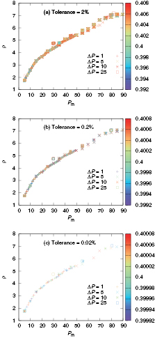
Figure 2. Measured data of the density,  , as a function of the pressure
  during a compression run in a two-dimensional GEM-4 system of cluster forming particles at a target temperature of
  for different values of
  , as specified in the legend. The symbols are colored according to the instantaneous temperature of the system (see colour code on the right-hand side). Panels (a), (b) and (c) show only those data for which
  is smaller than 0.02, 0.002 and 0.0002, respectively.
Download figure:
Standard image High-resolution imageWe come back to figure 1 and focus now on the observation that curves in the ( )-plane that collect data along different runs have different slopes. In an effort to provide a deeper insight into the mechanisms behind those processes that occur along these branches, we recapitulate the two principle mechanisms of how a cluster crystal reacts to a change in volume: (i) shrinkage/growth of the lattice constant, a, which is accompanied by a shift of the position of the main peak of the radial distribution function,
  , of the system towards a lower/higher r-value; (ii) deletion/creation of new lattice positions, reflected by an increase/decrease of the average cluster occupation,
  ; this quantity is obtained via a cluster analysis of the particle configurations, as specified in the appendix of [18].
We have displayed the data for  as a function of
  along the compression, the expansion and the 'new' compression runs in figure 3 in two different representations: (i) in the main panel the
  -data are colour coded according to their corresponding
  -value; (ii)
  -results in the inset are coloured according to the type of runs, i.e. data from compression and 'new' compression runs are displayed as red symbols, while the results from expansion runs are coloured in blue, thereby allowing the reader to establish a connection from these data to those in figure 1.

Figure 3. Average cluster occupation,  , as a function of the density in a two-dimensional GEM-4 system at a target temperature of
  during compression and expansion runs, imposing
  (compression runs) and
  (expansion runs). The symbols are coloured according to the
  value (see colour code on the right-hand side). The dotted, solid and dash-dotted lines specify the compression, the intermediate (lower, middle and upper), and the expansion branches, respectively. In the inset we display the same data, now results originating from compression runs are marked by red symbols, while the data stemming from the expansion runs are shown as blue symbols. The black circles mark the starting points of the expansion and of the new compression runs, the arrows indicate whether it is a compression (arrow pointing to the right) or an expansion (arrow pointing to the left).
Download figure:
Standard image High-resolution imageSurprisingly, the reactions of  and of
  on a compression or an expansion of the system help us to classify the different branches of data as functions of
  into three categories:
- 1.Compression branches (dashed line): along these branches
 increases linearly with the density. After an initial decrease for small densities, assumes an essentially constant value of up to high densities. This value corresponds to the minimum value that was observed in [18] in the compression experiments presented there;
 - 2.Expansion branches (dash–dotted line): these data were extracted during the final parts of the expansion runs, i.e. (). Along these branches shows again a linear dependence on the density, although with a larger slope than along the compression branches. Similar to along the latter branches, we observe a small variation of at small densities; a similar observation is made at rather high densities; however, over a large density range assumes a constant value of ;
- 3.Intermediate branches (solid lines) data along these branches stem either from the 'new' compression runs or from the initial part of the expansion runs (i.e.). As remains constant along these branches no cluster merging or splitting events occur. These sets of data connect the compression and the expansion branches, thus varies between and .


We summarise our observations as follows: if an ordered system of GEM-4 particles is compressed or expanded, the two fundamental reaction mechanisms of the system are completely decoupled and they obey the following scheme: (i) as an immediate reaction on compression/expansion the lattice spacing a of a cluster crystal is reduced/enhanced; it varies within a range ![$\left[d_{\text{nn}}^{\text{max}},d_{\text{nn}}^{\text{min}}\right]$](https://content.cld.iop.org/journals/0953-8984/27/32/325102/revision1/cm516704ieqn102.gif) while
while  remains constant; according to our above nomenclature, the system 'moves' along an intermediate branch; (ii) once the system has reached a state where
  , further compression will induce cluster merging processes [18]: the required volume reduction is effectuated by deleting lattice positions via cluster merging events (i.e.
  increases), while keeping the lattice spacing constant fixed at
  ; for this part of the compression process the system 'moves' along a compression branch; (iii) alternatively, if the system—once it has reached a state where
  —is further expanded, the considerably increased inter-cluster distance will reduce the repulsion among the clusters, and consequently the aggregates will start to split: the larger available volume will be filled by an increased number of newly created, but smaller clusters (i.e.
  decreases), while keeping the lattice spacing constant; for this part of the expansion process the system 'moves' along an expansion branch.
3.2. The quest for the equilibrium state
We now return to the question of how we can obtain in our experiments the density value that corresponds at a given pressure to the density that one would obtain from the equation-of-state of the system (i.e. the equilibrium state). So far, we can summarise our observations as follows: we obtain—depending on the protocol of our compression and expansion processes—different results for  , a and
  for a given
  -value; thus, we can conclude that the system is driven by the different processes into metastable states that are separated from the equilibrium state by large energetic barriers. To surmount these, we launch several annealing processes at constant
  , hoping we will recover in this manner an equilibrium state in the system. The starting configurations for the different annealing runs are selected from state points along the compression, expansion and intermediate branches.
During the annealing processes we keep the target pressure constant and increase the temperature until the system melts; then we cool the system down to the desired target temperature  . We hope that the energy that is introduced into the particles via the heating process allows the system to overcome the energetic barrier that separates the metastable states from the equilibrium state. If these annealing runs indeed lead to the equilibrium state, we expect all these processes (that start for a given
  -value from different
  -values) to end up at the same density, which we identify as the equilibrium density at this pressure value, i.e.
  . In total we have performed annealing runs at
  and 80.
In figure 4 we show the data for the measured density as functions of  for three annealing processes: they have been launched from state points that are characterised by
  and are located (i) at the compression branch (red symbols, initial density value of
  ), (ii) the middle intermediate branch (green symbols,
  ) and (iii) the upper intermediate branch (blue symbols,
  ). The
  -values are marked by grey rectangles and the final value of the density after the annealing process
  is marked as a purple circle.

Figure 4. Left panel: measured data of the density as a function of the temperature  for different types of annealing processes of a two-dimensional GEM-4 system of cluster forming particles, launched at
  ; these runs have been launched from the compression run (symbols in red), and from the middle (symbols in green) and from the upper (symbols in blue) intermediate branches (see text). The starting points of the respective runs are indicated by a rectangle. At
  ,
,  is switched
  to
to  . The density values measured at the end of the respective runs are marked by a violet circle. Right panel: snapshot of the system at
  .
.
Download figure:
Standard image High-resolution imageDuring the initial heating, the sets of data of the compression branch and of the middle intermediate branch merge at  and follow for the rest of the annealing process the same
  -curve. The results from the upper intermediate branch merge with the other sets of data at
  ; by a visual inspection of the particle configurations we can conclude that at this temperature the nanocrystal begins to melt. These annealing processes are stopped as the system reaches a temperature of
  , a typical snapshot of a particle configuration taken at that instant is shown in the right panel of figure 4, providing evidence that the system has completely lost its ordered structure. Now the increment in temperature,
  , is reversed from
  to
to  and the three sets of data follow during the subsequent cooling run essentially the same curve; eventually they reach a final, common state whose density is marked in figure 4 as a violet circle; obviously this value corresponds to the density of the equilibrium state,
  .
.
This protocol of annealing processes was repeated for different pressure values, namely for  and 80; the corresponding sets of data, displayed in the (
 )-plane are similar to those obtained for
  (and shown in figure 4). Each of these annealing runs carried out for a given
  leads to the desired
  -value. These density data (corresponding to
  , shown in purple) are summarised in figure 5, where, in addition, the original data for the density,
  , as obtained from the compression (light-red symbols) and from the expansion (light-blue symbols) runs are shown (see figure 1). The respective
  -values are plotted with dark-grey asterisks. The curve that connects as a function of
  the
the  -data represents at
  the equation-of-state, i.e.
  .
.

Figure 5. Measured data for the density,  , as a function of
  as obtained in compression (symbols in light-red) and in expansion (symbols in light-blue) processes of a two-dimensional GEM-4 system of cluster forming particles at a target temperature of
  . The dark-grey asteriks denote the starting points of the annealing processes: during such a process the pressure of the system is kept constant while the temperature is first raised until the system has melted and is then decreased down to the target value
  . The data shown by violet symbols denote the value for the density as it is measured at the end of the respective runs.
Download figure:
Standard image High-resolution imageOf course, the final answer if the obtained state indeed corresponds to an equilibrium state can only be given via additional free energy calculations. However, due to the high numerical costs for our different types of compression, heating and annealing runs we postponed additional free energy calculations (which themselves would have been rather time consuming) to future investigations on this system.
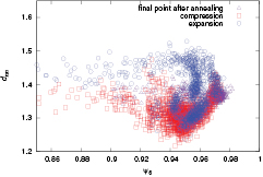
Our conclusions are supported by a structural analysis of the systems, putting again focus on  : we have investigated the correlation between the average distance of two neighouring clusters,
  , and the hexagonal order parameters,
  . The latter one is defined as (see [21])

where nj denotes the number of nearest neighbours of cluster j, and  the angle between the line connecting cluster j and its nearest neighbour k with a fixed axis. By definition,
  attains a value of 1 for a perfect hexagonal arrangement, while we typically found
  for the disordered liquid state.
In figure 6 we show this correlation between  and
and  , considering all the expansion (red symbols), compression (blue symbols) and annealing (violet symbols) runs, as well as all pressure values Prmm. We observe that during the compression and the expansion runs the maximum value of the order parameter obtains values of
  while after the annealing processes we obtain
  : thus, we conclude that annealing is able to heal out lattice defects in the cluster crystal. The maximum value obtained for
  corresponds to a nearest neighbour distance of
  which we thus consider the lattice spacing of the equilibrated state. This result differs from the corresponding value predicted density functional theory calculations (i.e.
  ); we attribute this difference to the fact that we are investigating a nanodroplet of finite size and not a bulk system.
Figure 6. Correlation between the average distance of two neighouring clusters,  , and the hexagonal order parameters,
  during compression runs (symbols in light-red) and expansion runs (symbols in light-blue) a two-dimensional GEM-4 system of cluster forming particles at a target temperature
  . The symbols shown in violet denote results as obtained at the end of the different annealing runs.
Download figure:
Standard image High-resolution image
4. Conclusions
In this contribution we have investigated a two-dimensional nanodroplet of ultrasoft, cluster forming particles that is surrounded by a layer of ideal gas particles. By varying the number of particles in this reservoir and by changing their velocities we can impose a target pressure and a target temperature on our nanodroplet.
Straightforward applications of compression runs on the system (i.e. keeping the temperature fixed at a target value  while systematically increasing the pressure by an increment
  ) transform an originally disordered system into a cluster crystal, i.e. a hexagonal arrangement of clusters of overlapping particles. This system is obviously not in an equilibrated state: this fact becomes evident in subsequent expansion runs (i.e. keeping
  fixed and applying now a negative pressure increment
  ) that lead—in dependence on the respective initial particle configurations—to states that differ in their densities,
  , from the corresponding
  -values that the system had assumed during the preceding compression run.
By systematically launching alternating sequences of compression and expansion runs in different sections of the investigated pressure range we provide evidence that these differences in the densities are not related to a dynamic lag. By analysing the evolution of the cluster occupancy and of the lattice constant of the cluster crystal along these processes we extract the following typical reaction scheme on compression and expansion of systems of ultrasoft particles: (i) immediately after compression/expansion the lattice spacing is reduced/enhanced until it assumes a characteristic, limiting value; (ii) once this value is reached, the averaged cluster occupancy (which remained constant so far), compensates for this spatial rearrangement by an decrease/increase in the cluster size.
In an effort to provide a route of how to reach the equilibrated state of the system with our setup we have introduced additional heating and annealing runs, i.e. keeping now the target pressure,  , fixed and varying the temperature via a positive or negative temperature increment
  , respectively. Selecting different starting configurations (each being characterised by its respective density value) at a fixed pressure, we could show that heating runs (until the system completely melts) and subsequent annealing processes lead to final states that have—irrespective of the density of the starting configuration—the same
  -value; we identify this density as the equilibrium density,
  , for this particular target pressure and target temperature.
Of course a complete analysis if the obtained states do represent equilibrium states would require additional free energy calculations, which would provide a final, unambiguous answer on this issue; due to the high numerical cost of the required, additional investigations we have refrained from this type of analysis. On this occasion we should also state that the strategy we used for our investigation takes benefit from the (presumably) continuous nature of the phase transition in the two-dimensional version of the system [22].
Acknowledgments
We thank A Nikoubashman (Princeton), M Grünwald and C Dellago (both Wien) for their helpful discussions. This work has been supported by the Marie Curie ITN-COMPLOIDS (Grant Agreement No. 234810), by the Austrian Science Fund (FWF) under Proj. Nos P23910-N16 and F41 (SFB ViCoM), and by the WK 'Computational Materials Science' of the Vienna University of Technology. Computational resources from the Vienna Scientific Cluster are gratefully acknowledged.