

Abstract
A recent comparison of the frequencies of a pair of optical clocks based on the 674 nm 2S1/2–2D5/2 optical clock transition in 88Sr+ has highlighted the need to understand factors affecting frequency instability. We have developed statistical models to show that our clock is capable of reaching the quantum projection noise limit; for our clock using 100 ms probe pulses, this is ∼3 × 10⁻¹⁵/√τ. However, this optical clock uses atomic transitions with a linear Zeeman shift, which can lead to a degradation in stability in the presence of magnetic field noise. We show that this generally leads to an increase in white frequency noise, even in cases dominated by magnetic field flicker or random walk noise. By taking into account both the quantum projection and magnetic field noise we are able to explain our observed frequency instabilities. This analysis will relate to any optical clock with a linear Zeeman shift where cancellation of this shift is achieved by interrogating pairs of components. Furthermore, implementing automatic control of lasers and minimization of micromotion requires pausing of the frequency servo occasionally; this leads to only a small degradation of frequency stability.
Export citation and abstract BibTeX RIS
1. Introduction
Optical clocks based on narrow linewidth forbidden transitions in single laser-cooled trapped ions offer improved stability and accuracy compared to microwave standards. Optical clocks using different ions are being developed worldwide, for example based on transitions in 27Al+ [1], 199Hg+ [2], 171Yb+ [3, 4], 115In+ [5] and 40,43Ca+ [6, 7]. Optical clocks based on a quadrupole transition in 88Sr+ are being characterized at the UK National Physical Laboratory (NPL) [8], the National Research Council (NRC) in Canada [9, 10] and also at MIKES in Finland. In this paper, we discuss the limitations to the frequency stability of our strontium ion clock at 674 nm, taking into account the observed linewidths and quantum jump rates. This can be explained by considering the statistical contribution of the lock to the ion, together with the effect of ambient magnetic field instability.
The 88Sr+ optical clock is based on the 5s2S1/2–4d2D5/2 electric quadrupole transition at 674 nm in a single laser-cooled strontium ion. Two independent traps are used and the frequency stability and reproducibility is determined by two-trap comparison. An ion is confined in an end-cap trap [11], which is driven with an RF voltage at a frequency of 14 MHz. The trap is placed between three pairs of magnetic field coils to null the ambient dc magnetic field and provide an additional bias field of ∼7 μT. Two-layer mu-metal shields reduce the effect of fluctuating magnetic fields, particularly those generated by nearby power supplies at the UK mains frequency of 50 Hz.
The ion is cooled using light at 422 nm which is provided by a frequency doubled diode laser at 844 nm (figure 1). A 1092 nm custom-made distributed feedback (DFB) laser is used to clear the ion out of the metastable 2D3/2 level. A second DFB laser at 1033 nm drives the 2D5/2–2P3/2 transition (figure 1). This laser is normally shuttered to the 'off' position, but light can be admitted to the trap under computer control when the ion has been observed to make a transition to the 2D5/2 level. The 1033 nm radiation rapidly returns the ion to the cooling cycle, minimizing the dead time between interrogations of the ion at 674 nm and hence reducing the time taken to lock to a Zeeman component. During each probe cycle, the 1033 nm radiation is turned off once 422 nm fluorescence is re-established.

Figure 1. Partial term scheme of 88Sr+, showing the cooling transition at 422 nm, de-populating laser transition at 1092 nm and the transition at 1033 nm needed to take the ion back from the 2D5/2 state into the cooling cycle. The 2S1/2–2D5/2 optical clock transition at 674 nm is also shown.
Download figure:
Standard image High-resolution imageThe 674 nm probe laser light is generated by an extended cavity diode laser locked to a high finesse ultra-low expansion optical cavity. Typically, 50 ms probe pulses are used with 20 Hz transform limited linewidths being observed in both traps. The choice of probe pulse length is limited partly by our clock laser instability and also the ion heating rate, typically 1–4 quanta/ms for our two traps [8]. Acousto-optic modulators are used to bridge the frequency interval of ∼90 MHz between a cavity resonance and the strontium ion 674 nm transition frequencies in the two traps. Full details of the interrogation cycle including the sequence of cooling and probing the ion on pairs of Zeeman components are described in [12, 13]. The locks of the probe and cooling lasers to their respective cavities, together with the drift of the two DFB lasers, are monitored and corrected as necessary under computer control [12]. Micromotion monitoring and automatic minimization in three non-coplanar directions in both traps has also recently been implemented. Pausing the frequency servo to the ion to make checks of the micromotion or the status of the laser locks to the cavities can cause a further small increase in frequency noise. However, we show that the resulting increase in instability is not significant.
2. Frequency stability prediction using a statistical model
The 88Sr+ 2S1/2–2D5/2 optical clock transition has a linear Zeeman shift and determination of the unperturbed centre of the Zeeman manifold is achieved by locking to different pairs of components symmetrically placed around the centroid [13]. The ion is interrogated via a pulse of probe laser radiation of duration τp. The number of quantum jumps is measured at two frequencies; one higher (ωH) and one lower (ωL) than the centre of each Zeeman component. If the centre frequency offset between the ULE cavity and ion transition is ωi after i servo cycles  then the frequency correction ωi+1−ωi at the (i + 1)th cycle is given by:

In this equation, the number of observed quantum jumps at frequencies ωH and ωL are n1 and n2 respectively. The primary gain of this frequency correction is denoted by gp. For the servo, we also need to set the dither frequency  ; typically this is set to the observed transition full width at half maximum (FWHM) linewidth. To take into account linear ULE cavity drift, a secondary gain is introduced:

The time interval Δt is measured between the current set of interrogations of the ion and those of the previous servo cycle. The frequency drift si, calculated after each servo cycle, is adjusted to make the time-averaged quantum jump imbalance  zero. This averaging period can be adjusted (typically 2 min is chosen) and also the secondary gain gs that relates subsequent iterations of the parameter s to
  (i.e.
(i.e.  ).
).
The laser servo to the ion and the resulting frequency stability for a two-trap comparison can be modelled using a random number generator with a binomial probability distribution [14, 15] to simulate the quantum jumps. For Rabi interrogation of the ion, the excitation probability (P) is given by:
In equation (3), the Rabi frequency is ΩR and the laser is detuned Δω from line centre. At low intensity (i.e. less than the saturation intensity) using a rectangular probe pulse of length τp and for a laser linewidth much less than 1/τp, the mean number of quantum jumps  can be written as:

In equation (4), n0 is the peak number of quantum jumps at line centre (i.e. when Δω = 0), and the observed transition FWHM is ∼0.89/τp.
The model was checked using experimental data from two traps, using 40 probe pulses at each frequency step, a primary gain gp/2π = 10 and pulse lengths of 40 ms, corresponding to transform limited linewidths of 22 Hz. The laser was locked to a single pair of ΔmJ = 0 components and our previously reported results [12] show a single trap relative frequency instability of 1.6 × 10⁻¹⁴/√τ for an averaging time τ. Under these same lock conditions, the model suggests that the limiting frequency instability should be 1.2 × 10⁻¹⁴/√τ, in reasonable agreement with the observed value. This limiting instability obtained with our statistical model can also be compared with the quantum projection noise limit for Rabi excitation, which is approximately [16]:
For a maximum excitation probability of pmax = 0.4 at 674 nm, probe time of τp = 40 ms, a deadtime (i.e. the time taken to observe whether the ion is fluorescing) of τd = 30 ms and Fourier transform limited linewidth of Δω0/2π = 22 Hz, this gives a predicted instability of 1.3 × 10⁻¹⁴/√τ, close to our modelled value. However, our model has the advantage of allowing us to also include the effect of changing servo parameters for our specific algorithm and also demonstrates that the algorithm is capable of achieving instabilities close to the quantum projection noise limit. Equation (5) assumes that the clock laser has a low frequency instability; for our system this has been determined from the beat between two similar systems [17]. This shows a beat linewidth of ∼2 Hz at 1 s, broadening to ∼6 Hz at 30 s, corresponding to single laser linewidths of ∼1 Hz and 4 Hz respectively. The laser instability is ∼2 × 10⁻¹⁵ after removal of a linear drift, close to the thermal noise limit for our cavity. In our system, where 40 probe pulse sequences are observed at a given 674 nm laser frequency, the servo loop time of the laser lock to the ion is τ = 11 s. On this timescale, the quantum projection noise limit is 4 × 10⁻¹⁵ and the cavity thermal noise does not therefore contribute significantly to our observed instability.
Equation (5) also provides an estimate of the limiting quantum projection noise for a laser locked to a single strontium ion. However, to achieve this, we need to drive ions into the 2D5/2 state with near 100% probability (i.e. pmax ∼ 1). This requires a new trap design with lower ion heating rates to allow near-coherent excitation into the 2D5/2 level [14]. Lower heating rates will also allow use of longer probe pulses to provide a narrower transform limited transition linewidth. Optical pumping will be required to drive ions into the correct Zeeman ground state for each clock laser probe pulse. Equation (5) then predicts a limiting single-trap instability of ∼3 × 10⁻¹⁵/√τ for 100 ms probe pulse lengths. For a servo loop time of ∼11 s, this instability corresponds to 9 × 10⁻¹⁶ and so we will also need to improve the clock laser performance; this could be achieved by using silica rather than ULE mirrors or longer spacers [18]. Magnetic field noise can potentially degrade this figure further and this is discussed in the next section.
Frequency locking to a single Zeeman component pair does not allow cancellation of the quadrupole shift or tensor components of the Stark shift [19, 20]. In order to evaluate the quadrupole shift, we need to probe three pairs of Zeeman components with different values of mJ of the 2D5/2 state. This necessarily involves the ΔmJ = ±2 Zeeman components that are 5 times more sensitive to magnetic field noise than the ΔmJ = 0 transitions. Zeeman component switching can therefore be expected to produce larger frequency instabilities because the clock frequency is more sensitive to magnetic field changes, although the systematic error from quadrupole and tensor Stark shifts is eliminated. In our strontium ion trap, we have demonstrated single-trap Allan deviations using Zeeman component switching of 2.2 × 10⁻¹⁴/√τ [8] for 50 ms probe pulses and a primary gain gp/2π = 7. However, under these conditions, the model predicts that a frequency comparison should have an instability of 1.1 × 10⁻¹⁴/√τ. The higher observed frequency instability with Zeeman switching may include contributions from increased sensitivity to magnetic field noise and uncertainty in the ratio between the three Zeeman component separations which will lead to a small frequency pull-in after each component change. Additional degradation in frequency stability might result from interruption of the frequency servo either to check the laser status or to check or minimize micromotion. These possible contributions to instability are discussed in the following sections.
3. Effect of magnetic field instability
Variations in the magnitude of the ambient magnetic field will degrade the observed trapped ion frequency stability as a result of changing linear Zeeman shift. Changes in magnetic field direction will also cause much smaller frequency changes via a varying quadrupole shift or tensor Stark shift. The ion acts as a sensitive magnetometer and so we can deduce the magnetic field instability from variations in the Zeeman separation between pairs of components. Magnetic field noise can arise from the six current controllers used to drive the magnetic field coils in our two traps. Alternatively, noise can result from ambient laboratory magnetic fields in our trap although these will be reduced significantly within the mu-metal shield. Figure 2 shows the magnetic field noise (σB) observed in our two traps via the Zeeman separation. This is observed to be largely flicker noise in character and varies slightly from day to day; typically σB ∼ 0.1 nT over timescales up to ∼3 h or ∼10 000 s. Over longer timescales, random walk magnetic field noise or field drift could dominate. To understand the effect of magnetic field noise on frequency instability, we consider these three types of magnetic field noise. This analysis will apply to any optical clock with a linear Zeeman shift where cancellation of this shift is achieved by interrogating pairs of components. The model will only need updating to allow for the different sensitivities to magnetic field of the clock transitions used. The effect of magnetic field noise will be greatest for alkali-like ion optical clocks with zero nuclear spin, such as 40Ca+ or 88Sr+. Linear Zeeman shifts of up to ±28 Hz nT−1 are observed on the clock transition for the Zeeman components used in 88Sr+. Several other ion and neutral atom optical lattice clocks are under investigation that operate on a J = 0–J' = 0 transition, but have non-zero nuclear spin (e.g. 27Al+, 87Sr). For these species, a small differential linear Zeeman shift between the ground and excited states arises from state mixing via the hyperfine interaction. The observed shift is typically over 1000 times smaller than that in 88Sr+. Magnetic field noise could still be a limiting factor for lattice clocks targeting instabilities below the 10−16/√τ level, if they are operated in magnetically noisy environments without any shielding.
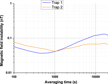
Figure 2. Magnetic field instability in our two strontium ion optical clocks measured from the Zeeman component separation of the 674 nm clock transition.
Download figure:
Standard image High-resolution imageServoing the 674 nm laser to the optical clock transition involves repeated interrogation and locking to the low frequency Zeeman component and then the upper frequency component [13]. A set of frequency offsets {ωi} from the ULE cavity frequency is obtained. This set starts at i = 1, so that interrogation of the lower frequency Zeeman component corresponds to odd values of i and even values correspond to the higher frequency component. The frequency shift of the ith Zeeman component is then proportional to (−)iBi, where the average magnetic field during the ith measurement is denoted by Bi. Measurements are separated in time by the servo loop period. For an optical clock based on a single Zeeman component, the frequency noise would directly reflect the ambient magnetic field noise. However, use of a pair of Zeeman components symmetrically placed around line centre modifies this effect.
The relationship between magnetic field and Zeeman shift for each of the three transitions is shown below in equation (6):
In these formulae, the magnetic field is denoted by B, the electron charge to mass ratio is e/me and Ω is the centre frequency of the Zeeman manifold. The values of the g factors for the 2S1/2 and 2D5/2 levels are denoted by gS and gD respectively. For LS coupling, gS = ge and gD = (ge + 4)/5, although the appropriate value for ge (the electron g-factor) will not exactly equal the free space value [21, 22]. For the three Zeeman components in equation (6), the dependencies of optical frequency (ω/2π) on magnetic field are approximately  5.6 Hz nT−1, ±11 Hz nT−1 and ±28 Hz nT−1 respectively.
Fitting the Zeeman separations for both of our traps from the results during the frequency stability measurements reported in [8] gives effective values for gD/gS. In our two traps, these ratios are observed to have slightly different values, giving rise to frequency differences at the level of a few Hz with a total Zeeman splitting for the ΔmJ = 0 transition of ∼10 kHz. This difference could be explained by the presence of a small vector Stark shift [23, 24]. This ratio therefore needs precise individual evaluation for both our traps to allow the software to predict accurately the frequency of different Zeeman transitions when jumping between components.
If we update the centre frequency of the manifold of Zeeman components Ω after the measurement of every component, then the noise introduced by the magnetic field will be proportional to  . Alternatively, we can update this frequency after both the low and high frequency Zeeman components have been measured. In this case, the noise introduced is proportional to {B2i – B2i−1}. In both cases, the measurement noise is related to the derivative of the magnetic field.
Updating the centre frequency either (a) after every Zeeman component frequency measurement or (b) after low and high frequency components have been measured gives new values for the centre frequency:


In equations (7a) and (7b), k is a constant including the g-factor (equation (6)) and {Ωi} is the set of Zeeman component frequencies extrapolated to zero magnetic field. The index i is an integer with i ≥ 1. For the case of linear magnetic field drift and updating the centre frequency after every Zeeman component measurement, we can write:

Here, Δt (≡ti+1–ti) is the constant period between measurements and the rate of magnetic field change is given by  . The sign change arises because alternate measurements probe firstly the low-frequency component and then the high frequency component. If we choose to update the centre frequency after both the high and low frequency Zeeman component measurements, then each measurement of the centre frequency is:

However, the measurement described by equation (9) has an inherent offset associated with it of  (where the bar denotes a time average) whereas the first measurement sequence (equation (8)) averages this to zero. Our ion traps are housed within dual layer mu-metal shields and the long-term linear magnetic field drift is typically <1 nT over 105 s or <10 fT s−1. This would correspond to a shift of only 2 mHz (i.e. 4 × 10⁻¹⁸ of the optical frequency) for a typical 10 s servo time on the ΔmJ = ±1 components.
We now consider the cases where magnetic field exhibits either flicker noise or random walk. It is straightforward to show [25] that the power spectral density of a parameter such as magnetic field (B) is related to the power spectral density of the time derivative ( ) by
) by  at a Fourier frequency ω. In [25], a relationship is stated for the case of optical phase, but is equally valid for other parameters. Also, in cases where the spectral noise density obeys a power law, (i.e.
  ) the Allan deviation is given by
  (for −3 ≤ α ≤ +1). However, when observing the magnetic field noise differentially, we should consider
  for which the Allan deviation is given by
  . For example, with random walk magnetic field noise (α = −2)
  is constant, corresponding to white frequency noise and the Allan deviation reduces as 1/√τ. Since
  is constant, introducing dead time between observations means that frequency noise will still average down as 1/√τ (i.e. it will retain a white frequency noise characteristic). This behaviour was confirmed numerically using noise data generated with a LabView routine and the results are shown in figure 3. This shows the resulting contribution to frequency noise where the random walk magnetic field noise is σB = (0.003 nT)√τ and the results are updated every servo cycle (equation (7a)). The assumed servo loop time (the time for the servo to the ion to update the frequency of one Zeeman component) is typically 11 s. If the centre frequency is updated after every servo cycle (equation (7a)), then the white noise contribution is (0.033 nT)/√τ; if frequency updates are after alternate cycles (equation (7b)) then the frequency update period is ∼22 s and the white noise contribution is √2 times larger, or (0.047 nT)/√τ. These two white noise contributions equal the random walk noise at the appropriate servo loop time of 11 s and 22 s respectively. Reducing this servo period by using fewer probe pulse interrogations at each frequency will reduce the contribution to frequency noise from random walk magnetic field noise.
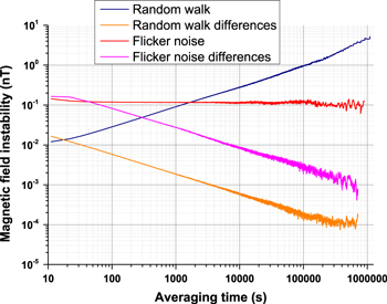
Figure 3. Modelling of the effect of flicker (σB = 0.1 nT) and random walk (σB = (0.003 nT)√τ) magnetic field noise on a strontium ion optical clock. The contribution to frequency noise in both cases is shown with the centre frequency updated after every servo cycle (equation (7a)). In both cases the frequency instability contribution reduces as 1/√τ (white frequency noise).
Download figure:
Standard image High-resolution imageThe case of magnetic field flicker noise (where α = −1) is less straightforward. A numerical simulation is shown in figure 3 with flicker noise generated using LabView to give σB = 0.1 nT, close to the observed value of figure 2. From the arguments previously presented, we would expect this to lead to flicker phase modulation, with σ ∝ 1/τ. However, the magnetic field noise is observed in a way that is not exactly the differential—either sign changes are introduced between observations or we must allow a dead time and only update the centre frequency after alternate Zeeman component interrogations. The effect of introducing dead time is to change the flicker phase character to white frequency noise [26] and the Allan deviation then reduces as 1/√τ rather than 1/τ. The effect of the sign change also has the effect of changing the noise character to white frequency noise. After a few (∼40) servo cycles with a magnetic field flicker noise of ∼0.1 nT, the contribution to the white frequency noise is (0.87 nT)/√τ for an 11 s servo period. In this case, the frequency noise contribution does not depend on whether the centre frequency updates are applied according to equations (7a) or (7b). The scaling between magnetic field and frequency will depend upon the Zeeman component selected.
From the modelling results presented, a 0.1 nT magnetic field flicker noise in the difference between the two traps will give rise to (0.87 nT)/√τ white noise. For Zeeman switching with equal interrogation times between the three components shown in equation (6), the average scaling between magnetic field and frequency is 15 Hz nT−1. The magnetic field noise will therefore contribute (13 Hz)/√τ to the frequency noise, or 2.9 × 10⁻¹⁴/√τ; for a single trap this equates to 2.1 × 10⁻¹⁴/√τ. When added in quadrature to the statistical noise of 1.1 × 10⁻¹⁴/√τ discussed earlier, this gives an expected frequency noise floor of 2.3 × 10⁻¹⁴/√τ, very close to the observed result of 2.2 × 10⁻¹⁴/√τ [8]. For the case where we lock only to the ΔmJ = 0 component, and assuming a similar magnetic field noise, the scaling is 5.6 Hz nT−1 and so the contribution to frequency noise for a single trap is (3.5 Hz)/√τ equivalent to 0.8 × 10⁻¹⁴/√τ. When added in quadrature to the 1.2 × 10⁻¹⁴/√τ predicted by the statistical model, this gives a total white noise level of 1.5 × 10⁻¹⁴/√τ. This is also close to the observed single trap frequency instability figure of 1.6 × 10⁻¹⁴/√τ [12].
4. Modelling the effect of pausing the frequency servo
We have shown that the statistical lock noise and ambient magnetic field noise together explain the observed frequency instability in our optical clock. The models presented explain the observed instabilities when locking either to the ΔmJ = 0 transition or when using all three Zeeman components. However, a long-term aim is to improve system reliability and automation that can require the software to pause the frequency control to the ion for a few seconds from time to time for diagnostic checks. These checks could include laser frequency and lock monitoring (including occasional lock reacquisition), ion re-loading and monitoring of the RF-photon correlation signal, with most of the monitoring time spent checking the correlation signal. During the period of these checks, the clock output is maintained but the laser is locked only to the ULE cavity, rather than also being steered by the ion transition. This section explores the effect of such interruptions on the observed frequency stability. Whereas such automatic monitoring can be expected to improve reliability and long-term system accuracy by better parameter control, this might be at the expense of degraded short-term frequency stability. We therefore need to understand how much monitoring time is permissible before it significantly affects frequency stability.
The level of micromotion is known to vary, particularly in the first few hours after ion loading [27] and increasing micromotion will reduce the quantum jump rate, thereby degrading frequency stability. For our standard, we have therefore implemented automatic micromotion control that requires the frequency servo of the clock laser to the ion to be paused to monitor and minimize the micromotion in three non-coplanar directions. These pauses place increasing demands on the stability of the magnetic field and also the linearity of the drift of the ULE cavity used to control the short-term stability of the clock laser. Although the software corrects for linear cavity drift, it will do this with an associated random error. This ULE drift error becomes a frequency error increasing with time during the period that the frequency servo is paused. Although this error is corrected once the correlation monitoring or servoing has been completed, there will be a pull-in period and we can therefore expect that the laser frequency instability will increase.
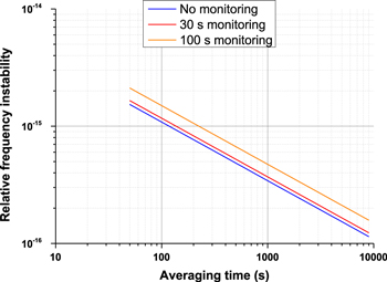
The results of modelling the necessary pauses in the frequency servo to the ion for issues such as micromotion monitoring or control are shown in figure 4. These results show the effect on the overlapping Allan deviation of pausing the servo for two 30 s and 100 s periods every 5 min. Whereas there is some increase in the level of white frequency noise, this can be kept at the <5% level if the correlation servoing and monitoring occupies no more than about 10% of the frequency servo time available (e.g. 30 s every 300 s). For these small monitoring periods, the increased instability is consistent with that expected by considering the increased time required to complete a given number of probe pulse interrogations. Typically, quantum jump rates can reduce by up to ∼20% within a few hours, resulting in a degradation of ∼10% in instability. Whilst the correlation servo slightly increases frequency instability, it prevents this larger instability occurring over timescales of a few hours as a result of a reducing quantum jump rate.
Figure 4. Effect of pausing the frequency servo of the clock laser to the ion, for example to make micromotion correlation measurements. The duration of the pauses indicated are over a timescale of 5 min. Provided these periods are less than about 10% of the total servo time, we conclude that there is little resulting degradation in frequency stability.
Download figure:
Standard image High-resolution image
5. Conclusions
We have demonstrated a model to allow prediction of the frequency stability for a 88Sr+ trapped ion optical clock at 674 nm. Previously published frequency stability data agree well with this model both for single Zeeman component and three-component locking. The dominant contributions to frequency noise are the statistical noise arising from the lock to the ion and the effect of ∼0.1 nT of magnetic field flicker noise assuming an ∼11 s servo loop time for the lock of the laser to the ion. We have demonstrated that, although the ambient magnetic field has flicker noise, the effect of this is to add to the white frequency noise of the standard. Random walk magnetic field noise is also expected to lead to additional white frequency noise.
The effect of magnetic field noise is most critical when interrogating the ΔmJ = ±2 transitions that have the largest frequency sensitivity to magnetic field noise. Our modelling and analysis should be relevant for any optical clock that has a linear Zeeman shift that is cancelled via the interrogation of a pair of components although this effect is most important in clocks with large linear Zeeman shifts.
We have also presented numerical simulations to demonstrate the effect of occasionally pausing the frequency servo for ion monitoring and diagnostic purposes. However, this can be set at a level that does not contribute significantly to the overall level of frequency noise.
These results can be used to specify the requirements for achieving the quantum projection noise limit of ∼3 × 10⁻¹⁵/√τ in a strontium ion clock. In order to achieve this, we have discussed the improved specifications required for our traps, the clock laser and magnetic field shielding. Reducing the number of probe pulse interrogations from 40 to 10 with the servo loop time reduced by a factor of four, will halve the noise contribution from the magnetic field to ∼1 × 10⁻¹⁴/√τ. Finally, further mu-metal shielding and improvements to the field coil drivers is needed to reduce the magnetic field noise from σB = 0.1 nT to σB = 0.02 nT to contribute only 2 × 10⁻¹⁵/√τ to the frequency noise. With all these improvements, we expect to achieve the limiting quantum projection noise for a single trap of ∼3 × 10⁻¹⁵/√τ.
Acknowledgments
This work was funded by the UK Department for Business, Innovation and Skills, as part of the National Measurement System Electromagnetics and Time programme and also by the European Metrology Research Programme (EMRP). The EMRP is jointly funded by the EMRP participating countries within EURAMET and the European Union. The authors would also like to thank members of the NPL Time and Frequency group for support and discussions.