


Abstract
The 3D photodissociation dynamics of Li Ne system is investigated by quantum calculations using the multi-configuration time-dependent Hartree (MCTDH) method and by classical simulations with the trajectory surface hopping (TSH) approach. Six electronic states of A' symmetry and two states of A" symmetry are involved in the process. Couplings in the excitation region and two conical intersections in the vicinity of the Franck–Condon zone control the non-adiabatic nuclear dynamics. A diabatic representation including all the states and the couplings is determined. Diabatic and adiabatic populations calculated for initial excitation to pure diabatic and adiabatic states lead to a clear understanding of the mechanisms governing the non-adiabatic photodissociation process. The classical and quantum photodissociation cross-sections for absorption in two adiabatic states of the A' symmetry are calculated. A remarkable agreement between quantum and classical results is obtained regarding the populations and the absorption cross-sections.
Export citation and abstract BibTeX RIS
1. Introduction
Analyzing the relaxation dynamics is an important subject of photophysics and photochemistry. Since the existence of bright light sources in the visible and UV range, it is possible to excite selectively a given electronic state of a molecular system and to analyze the various rearrangement channels, which reflect the electronic structure of the molecule along its deformation path. In many cases, the relaxation induces large motion of the nuclei where the various adiabatic electronic states can be significantly coupled. This is particularly true when conical intersections exist among the excited states, the dynamics at the intersections controlling the issue of the fragmentation through non-adiabatic transitions. The determination of the electronic structure of complex molecules is a very challenging task in such a case. The exact location of the intersections as well as the dynamical couplings are usually quite difficult to obtain accurately. It is thus desirable to have at our disposal model systems, computationally simple enough and yet experimentally achievable, to investigate the relaxation dynamics of photoexcited molecules. Alkali dimers (A2) constitute a particular class of molecules often studied in quantum chemistry, which fulfil this criterion when they are coupled to a rare gas (RG) atom by weak Van der Waals interaction.
The interest for these molecules comes from the simplicity of their electronic structure, which is closely related to the electronic structure of the hydrogen molecule. Such a simplicity is inherited from the one of the alkali atoms, which can be described as a one electron system on top of a relatively inert closed shell core. Moreover, the molecules and clusters made of alkali atoms exhibit dipole transitions in the visible range with large oscillator strengths, which allow experimental studies of the excited states by means of laser excitation.
Each of the corresponding cations, A2+, is representative of the most elementary molecule made of two singly charged nuclei bound by a single electron. When varying the atomic number along the first column of the periodic table, the electronic binding energy diminishes, while the fine structure splitting increases. These slight changes are going to affect the motion of the molecule in its excited state, as observed in their ro-vibrational spectrum [1–3]. Each A2+ is thus a paradigm of the molecule concept, which can be used to investigate the relaxation dynamics in the presence of a weak perturbation.
Among the homonuclear alkali dimers, Li2+ takes a specific place. The potential energy curves of the excited  and
and  states cross in the Frank–Condon (FC) area which makes this system very interesting to investigate. When the Li2+ dimer is bound to a rare gas atom, the resulting weak external perturbation couples the potential energy surfaces (PES) correlated with the
  and
and  states and the non-avoided crossing in the free Li2+ dimer becomes a conical intersection in the Li2+-RG trimer, which shape is completely determined by the position and the nature of the rare gas atom. These trimers form thus, a class of molecules particularly well suited to the study of relaxation dynamics in the presence of conical intersections. Besides the simplicity of their electronic structure alkali cationic dimers form bound systems with rare gas atoms and clusters, while neutral molecules do not bind with the lightest rare gas because of the large zero point energy motion (ZPE). Such Li2+-RG systems are thus experimentally achievable and could provide a wealth of information regarding non-adiabatic relaxation dynamics, by changing the conditions like the nature of the rare gas bound to Li2+ or the presence of weak external electric or magnetic fields.
The electronic structure of alkali clusters can be computed accurately by means of core polarization pseudopotential (CPP). The interaction of the valence alkali electron with rare gas atoms can be also accurately represented by means of 0-electron CPP [4]. Combining these pseudopotentials, we obtain an accurate model of the excited states of clusters made of alkali and rare gas atoms, which is remarkably numerically efficient.
Classical and quantum frameworks can be used to theoretically examine multidimensional non-adiabatic dynamics and these methods are often complementary. The classical methods can deal with very large systems with long propagation time but obviously cannot show quantum effects such as possible interferences, vibrational quantization or tunneling effects, whereas time-dependent quantum methods are rather dedicated to smaller systems and rapid dynamics.
In the present paper we investigate in detail the relaxation dynamics of Li2+Ne trimer under excitation from the ground state in the Frank-Condon area. We perform our quantum analysis in the framework of the MCTDH [5–10] method using the Heidelberg package [11], which allows us to take into account the quantum effects associated to the motion of the light atoms constituting the trimer. MCTDH is a powerful algorithm designed to solve quantum molecular dynamics of large systems, but it is also very useful for solving low-dimensional systems when large primitive basis based on discrete variable representation are required. This is typically the case for photodissociation processes where the wavepacket must eventually be propagated to large values of the scattering coordinates and for which an exact quantum wavepacket calculation becomes rapidly impracticable. MCTDH has been successfully applied to various photodissociation processes [6, 12–25] and to multimode non-adiabatic dynamics [26–42]. In this work, we also establish a link with previous studies [4, 43, 44] by performing a simulation by means of classical molecular dynamics with trajectory surface hopping (TSH) approach [45–47]. By contrast to the quantum approach, this method does not require any approximate diabatization and it allows us to follow the dynamics over long time, which is particularly convenient to identify the atomic arrangements in the exit channels. Its limitations are well known [45–47]. They are mainly due to the approximate treatment of the propagation around the conical intersections, and to a lesser extent to the neglect of the vibrational states quantization.
2. PES and couplings
2.1. Molecular states
For the bare Li molecule there are two adiabatic states, namely, the
  (
( ) and
) and  , correlated with the Li
  +Li+ asymptote and six adiabatic states, namely, the
  , two degenerated
  components, two degenerated
  components, and the
  , correlated with the Li
  +Li+ asymptote (figure 1). Among these states, only the
  , and the
  states can be reached by a dipolar transition from the
  ground state. For Li
 , the
, the  PES is purely dissociative, while the
  are bound states. The
  PESs cross the
  in the Frank-Condon region for Li-Li interatomic distance
  au and the
  around
  au, as it can be observed in figure 1.
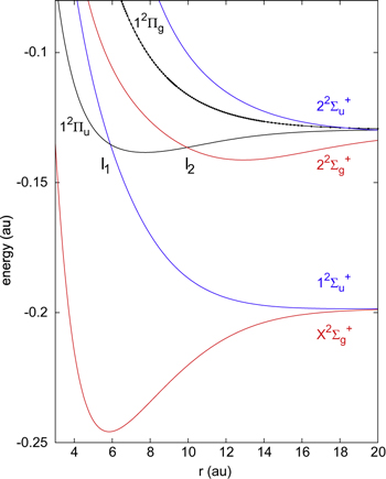
Figure 1. Ground and excited potential energy curves of Li2+ molecule. The curves were obtained by means of 1-electron CPP approach [43].
Download figure:
Standard image High-resolution imageWhen adding the Ne atom, several modifications of the electronic structure take place. First of all, the symmetry of the system is lowered from D to C
to C . There are six states in the A' subgroup correlated with the
  ,
,  ,
,  ,
,  ,
,  and
and  states of the bare Li2+ molecule, and two states in the A" subgroup correlated with the
  ,
,  states of the bare Li2+ molecule. The latter have the valence π orbital perpendicular to the molecular plane (i.e. the xOz plane in the present case) and remains uncoupled from the states of the A' subgroup, as far as the rotation and fine structure effects are disregarded.
We consider the six energy states in the first symmetry subgroup A, where the above defined states are coupled among themselves. As a result, the crossing observed in the bare Li molecule between the
  and the
  states generates a first conical intersection labeled I1. Moreover, the crossing observed between the same
  and the
  states defines a second conical intersection labeled I2.
The presence of the Ne atom leads also to a spectral blue shift of the  −
−  transition. As discussed in a previous paper [44], this shift, common to all alkali systems, is due to the confinement of the
  orbital in the
  state at the equilibrium geometry of the ground state. As a result, compared to Li2+, the crossing I1 between the
  and
and  states is shifted towards larger distances, slightly outside of the FC zone.
2.2. Diabatization
Multi-dimensional non-adiabatic dynamics involves adiabatic PESs where the couplings, due to the kinetic energy, lead to multiple dissociative pathways. When the PESs intersect in conical intersections, the couplings become singular and it is therefore more convenient, in the quantum calculations, to move to a so-called diabatic representation where the electronic Hamiltonian is no more diagonal and where the couplings are due to the potential instead of the momentum-like operator. A diabatic basis has the advantage to represent the different states, which in this basis preserve their electronic character, with smooth functions of the nuclear distances and non-singular coupling terms. In classical trajectory-based approximations as the commonly used Tullyʼs TSH scheme, the non-adiabatic couplings induce hops between the adiabatic states and diabatization is not required.
For Li2+Ne molecule, the Ne atom represents a relatively weak perturbation. It is therefore possible to obtain a approximate diabatic hamiltonian by using the Li2+ molecular states of the D symmetry group. The fine structure effects like spin-orbit coupling are neglected here. The radial coupling between two states of different symmetry vanishes and the coupling between the
  and
and  states is negligible because of the large energy difference between these states. The angular coupling between
  and
and  states is neglected here like any other rotational effect. The diabatization is done as follows. We first built the adiabatic molecular states of the bare Li2+ molecule in the D
 symmetry group. The electronic structure is computed by means of core polarization potential, which reduces the problem to a one electron calculation [43]. The valence orbitals are represented with a basis set made of
  gaussian type orbitals (GTO) centered on each Li atoms. In a second step, we compute the eight lowest energy molecular states of the Li2+Ne molecule with a complementary basis made of
  GTO centered on the Ne atom. The standard procedure of projecting the Li2+Ne eigenstates onto those of Li2+ does not work well for short LiNe distances, because the overlap between the model eigenstates and the original ones becomes too small for the uppermost energy state. This means that the Li2+ eigenstates are significantly mixed with higher energy states not included in the model space. The only correct way to cure the problem would be to include more and more states. This approach is unfortunately unpractical and we simply build a quasi-diabatic model hamiltonian
  by substitution of the Li2+Ne eigenstates by their Li2+ counterpart, i.e.:
where  is the hamiltonian in the primitive GTO basis set and
  are the expansion coefficients of the bare Li2+ molecule in the primitive basis truncated to the basis function centered onto the Li atoms. For weak LiNe overlap the model hamiltonian is identical to the hamiltonain obtained by standard projection procedure. For more cramped geometries, the model hamiltonian provides a continuous quasi-diabatic extrapolation, well suited to wavepacket simulation. The diagonalization of the above model hamiltonian restores quite faithfully the adiabatic energies, except for very cramped geometries, which have a limited contribution to the relaxation dynamics explored here. We notice, however, a small shift of about 0.06 eV at equilibrium position for the second A' excited state (
 ) with respect to the reference adiabatic energy. We also mention here that there is a systematic shift of 0.11 eV with respect to previous calculations for all transitions because of an erroneous energy conversion factor in our previous work [4].
For the sake of clarity, the diabatic states, which keep during the dissociation their electronic configurations, are labeled  to
to  . They correspond, following the order at short range of the adiabatic states of the bare Li
 molecule (see figure 1), to the
  ,
,  ,
,  ,
,  ,
,  ,
,  states respectively. The adiabatic states are labeled
  to
to  in increasing order of energy in the Franck–Condon region area. The
  and
and  adiabatic states built initially respectively on the
  and
and  states of the bare Li
 molecule in the Franck–Condon region correlate with the lower Li
  + Li+ channel, while the
  to
to  adiabatic states built initially mainly on the
  ,
,  ,
,  ,
,  states of the bare Li
 correlate to the higher Li
  +Li+ channel. The order of the
  and
and  states changes when going from diabatic to adiabatic states in the FC area.
3. MCTDH framework
3.1. Wavepacket representation
In the time-dependent picture, the MCTDH method [5–11] combines the efficiency of a mean-field method with the accuracy of a numerically exact solution. The wavefunction is expanded as a linear combination of Hartree subproducts of single-particle functions (SPF) :
where f is the number of degrees of freedom (DOF) of the system,  denote the nuclear coordinates,
  the MCTDH expansion coefficients and
  the
the  SPFs associated with the degree of freedom κ. In large systems, coordinates can be combined together and treated as one 'particle'. The multiconfigurational nature of equation (2) results in a correct description of the correlation between the degrees of freedom provided the SPF basis set is large enough, or equivalently there is a sufficiently large number of configurations. The SPFs are represented on a time-independent primitive basis set with
  points for the
  degree of freedom:
The  are usually chosen as the basis functions associated to a discrete variable representation (DVR) or the fast Fourier transform (FFT). Each degree of freedom is associated with a small number of SPFs, which, through their dependence on time, allow to efficiently describe the entire process. The equations of motion derived from the Dirac–Frenkel [48, 49] variational principle form a set of coupled nonlinear differential equations of the first order. For non-adiabatic systems, that can not be described by a single PES and undergo conical intersections, the different electronic states have to be included in the calculations. In the so-called multi-set formulation, an extra DOF is added for each electronic state in the equation (2), with a different set of SPFs for each state. For our 6 electronic states, the wavefunction is then written as:

with each  expanded in the MCTDH form as:
In order to make the MCTDH method efficient, the Hamiltonian operator must be written as a sum of products of single-particle operators. The kinetic energy operator usually has the required form. For the potential energy operator, which does not have the necessary product form, there exists an efficient algorithm POTFIT [7, 9, 50] in the package [11], allowing to transform the potential for subsequent MCTDH calculations. For more details on the MCTDH algorithm we refer to the review papers [7, 9, 10].
3.2. Computational details
The calculations are carried out using standard atom-diatom Jacobi coordinates: r is the Li separation, R the distance between the center of mass of the Li
 molecule and the Ne atom and θ the angle between the two vectors
  and
and  . To reduce the lengths of the grids in the r and R modes, complex absorbing potentials (CAP) are employed [51, 52]. The grid lengths extend from 4.0 au to 26 au for r and from 5.0 au to 18.0 au for R. CAPs are located at r = 23 au and R = 15 au. Fast-Fourier-transform [53, 54] primitive-basis representations are used in the radial coordinates with 256 and 192 grid points in r and R respectively. In the angular θ mode, due to the symmetry, a restricted Legendre DVR is used with 180 points in the range [0,
  ].
].
3.3. Convergence and accuracy
Care was taken to study the convergence of the quantum results as a function of the number of SPFs. The rapid dynamics in the early-time region (see section 4.1), which, due to the repulsive character of the different states, involves a small part of the coordinate grids, can be correctly described with a relatively few number of SPFs (typically 3 to 7 in each mode). By contrast, for the slower dynamics in the region of the conical intersections and beyond, more SPFs were needed to obtain the convergence of the diabatic populations. The propagation until 700 fs was carried out with typically 15 SPFs in each mode for states 1d to 4d and 7 SPFs for states 5 and 6. Since in the multi-set formulation, the wavefunction has a component for each state (see equation 3), the diabatic populations equal to the norm of this component are straightforward to obtain. For the calculations of the adiabatic populations, we used one of the analysis tools of the MCTDH Heidelberg package [11]. Since the projection operator for the adiabatic states does not have the required MCTDH form, the adiabatic populations given by the expectation value of this operator are more difficult and long to obtain, especially as the calculations run over the primitive basis. The calculations can be accelerated by using an algorithm in which the one-dimensional grid-populations (1D-densities) are neglected when they are lower than a given threshold, but the results are, of course, less accurate. Here, a threshold of 10−10 was used in the short-time region, and a threshold of 10−12 was necessary to obtain enough accuracy in the long-time domain where the effects to show are very weak. The calculations are still very long and we did not calculate the adiabatic populations at every time-step.
4. Dynamical simulations
4.1. Quantum dynamics
The localization and the width of the initial wavepacket in the spatial arrangement of the atoms play a crucial role in the photofragmentation process. The vibrational ground state on the ground  electronic PES of Li
 Ne, is obtained by energy relaxation [55]. This state has a linear geometry where the initial distributions in the radial coordinates r and R and in the associated momentum are Gaussian-like, well localized around the equilibrium distance r = 5.83 au and R = 7.00 au. In the θ mode, the wavefunction is slightly delocalized having a full width at half maximum around 26 degrees. Following the Frank-Condon approximation, the vibrational ground state of the electronic ground state provides the initial wavefunction for solving the time-dependent Schrodinger equation on the coupled excited PESs.
Although, strictly speaking the diabatic states do not exist, the fact that they preserve their electronic character during the fragmentation renders the analysis of the dynamical mechanisms more convenient in the diabatic basis. It is the reason why the calculations are carried out for initial excitation at the center of the Franck–Condon region in both purely diabatic and adiabatic states. Moreover diabatic and adiabatic populations are presented. Since the 2a state preserves with more than 99,9% its  character, the results corresponding to the excitation in the 2a and 2d (
 ) states will be virtually identical. By contrast, in the
  symmetry corresponding to the equilibrium geometry, the 3d,
  , state is mixed with the 4d,
  state (21%) and to a lower extent to the 6d,
  state (0.4%) and to the 1d,
  state (0.02%). The 3a initial state is thus defined as a coherent superposition of the diabatic 3d, 4d, 6d and 1d states with the above corresponding weights. We have controlled that the coherent superposition defining the 3a state does not change significantly over the geometries covered by the initial wavefunction. Indeed, the maximum change on the weights was found equal to 6% over all coordinates in the full width at half maximum of the multi-mode wavefunction.
Figure 2 illustrates the short-time dependence (up to 300 fs) of the photofragment diabatic populations subsequent to absorption in the diabatic 3d state. The long-time dependence will be discussed below. Flux appears initially in the n = 3d state which corresponds, in the bare molecule, to the repulsive  state. The mixings, in the excitation region with the
  (4d) and
  (6d) states is observed in the instantaneous decay of the 3d population and in the increase of the 4d and 6d populations. The strong oscillations at short-time are Rabi-like oscillations. The frequencies and the amplitudes of these oscillations are governed by the behavior of the underlying potential curves and coupling elements over the short-time range of the photofragmentation. The inset in figure 2 depicts the early-time oscillations in the range 0–20 fs determined with a time step equals to 0.1 fs. Since, as discussed above, the PESs of the excited states conserve the repulsive character observed for the potential energy curves of the bare L
 dimer in the Frank–Condon region, the dissociation proceeds with a rapid elongation of the r (Li-Li) coordinate. Moreover, both radial R and angular θ coordinates vary. The system belongs thus to Cs symmetry rather than equilibrium C
 and all states are involved in the process. The initial 3d wavepacket evolves rapidly towards the conical intersection I1 and flux is transferred to the 2d and 5d states as evidenced in the decrease of the 3d populations and the corresponding increase in the 2d and 5d ones. About 25 fs are required to reach the conical intersection. The non-crossing in the 3d (
 ) and 2d (
 ) states populations indicates a rather diabatic passage through conical intersection I1 for the energy range included in the wavepacket. Finally, at larger time, around 40 fs, flux is increasingly transferred to the ground 1d (
 ) state. Due to the strong repulsive character of the 3d PES and since both 3d and 1d states correlate to the lower (Li
  Li+) asymptote, the wavepackets corresponding to the
  (3d) and ground
  (1d) states rapidly reach the CAP on the r coordinate to be finally absorbed (around 130 fs). The increase in the 4d population and the decrease in the 2d population, around 100 fs, are characteristic of the flux transferred out the
  state to the
  state when the wavepackets corresponding to these states undergo the second conical intersection I2 and finally, the flux is absorbed by the CAPs beyond 200 fs.
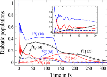
Figure 2. Time dependence of diabatic populations after excitation in the 3d state. States of  symmetry: solid line without symbols
  (1d), circle
  (4d). States of
  symmetry: line dots
  (3d), small dash
  (6d). States of
  symmetry: triangle up
  (2d), long dash
  (5d). The inset shows the Rabi oscillations in the short time range.
Download figure:
Standard image High-resolution imageIn figure 3, the population redistribution is displayed for initial excitation in the 2d ( ) state, which, in the excitation region corresponds to the adiabatic 2a state. Comparing with figure 2, we observe, a qualitative similarity in the early-time evolution except for the Rabi-like oscillations which, since the excited state is uncoupled, disappear here. The opposite variation in flux associated with the two n = 3d and 2d diabatic states still occurs. Since, however, the initial photoexcitation energy in the 2d state (3.02 eV) is lower than that for initial population in the 3d state (3.87 eV), the flux transferred out of this initially
  populated level is shifted in time. Now, about 40 fs (compared to 25 fs) are required to reach the conical intersection I1. This is also true for the redistribution in the 1d state which occurs now around 70 fs (compared to 40 fs) and for the time where the parts of the wavepacket corresponding to the
  (3d) and
  (1d) states are absorbed by the CAP on the r coordinate (around 170 fs compared to 140 fs). By contrast to excitation in the 3d state, there exists here a crossing between the fluxes in 2d and 3d states which indicates a rather adiabatic passage through the conical intersection I1. Moreover, one clearly observes, that beyond 200 fs, flux remains exclusively in the state 2d (
 ) state. The binding character of this 2d (
 ) state prevents the major part of the wavepacket from meeting the conical intersection I2, at least in time up to 300 fs, and transfer to the
  state is no more detectable. As already observed in
  clusters for low number m of Ne atoms [44, 56] the wavepacket is trapped in the 2d (
 ) state for some time, performing oscillations in the binding state which, in turn, should induce vibrational structures in the absorption spectrum. This point will be discussed in more details below in section 4.3. This effect occurs also for initial population in the 3d state, but, because of the energy distribution, it concerns solely an extremely small part of the wavepacket. The survival time of the wavepacket in the 2d state is controlled by the localization on the 2d PES of the conical intersections I1 with the 3d PES, and I2 with the 4d PES and by the diabatic couplings between the 2d state and both 3d and 4d states. Transfer of flux to these latter states can be observable in the long-time evolution. The inset in figure 3 displays the populations in the 3d and 4d states in the range 250 fs to 700 fs. We clearly see two oscillations when the wavepacket reaches the conical intersection I1, inducing transfer to the 3d state, and one oscillation when the wavepacket reaches the conical intersection I2 inducing transfer to the 4d state. Since the transfers are very weak, the scale in the populations is divided by 100. For both states, the population gradually increases at every passage through the conical intersections I1 or I2 and then decays when the wavepackets reach the CAPs in r and R coordinates, giving the observed oscillatory structure. We also observed a very low transfer in the 4d state due to the energy range contained in the wavepacket. The transfer processes slowly diminish the population in the 2d state which is still equal to 15% for t = 700 fs. This long-time dynamics of the fragmentation and the bound character of the 2d state can be illustrated by the time evolution (not shown here) of the one-dimensional (1D) probability densities in the different radial coordinates, showing back and forth in the well region.
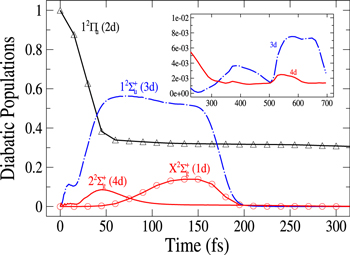
Figure 3. Time dependence of diabatic populations after excitation in the 2d (2a) state. States of  symmetry: solid line without symbols
  (1d), circle
  (4d). Line dots
  (3d). Triangle up
  (2d). For clarity, the populations in the 5d and 6d states, remaining weak, have been suppressed. The inset shows the longer time evolution of the 3d and 4d states.
Download figure:
Standard image High-resolution imageFigure 4 displays the diabatic populations for initial excitation in the adiabatic 3a state which could be populated in an experiment. Excitation occurs now predominantly in the 3d,  , state with a probability
  around 79% and to a lower extent in the 4d,
  state with a probability
  around 21%. This latter state, which is dipole-forbidden in the
  symmetry of the bare
  molecule becomes dipole-allowed in the initial
  symmetry of
  . Here, as before, the Rabi-like oscillations almost disappear. Moreover, we observe, a great degree of qualitative similarity for the dynamical processes with figure 2. However, since the photoexcitation energy (3.26 eV) is lower here than for excitation in the 3d state (3.87 eV), the coupling strength is different and the flux redistribution leads to different time evolution of the populations.
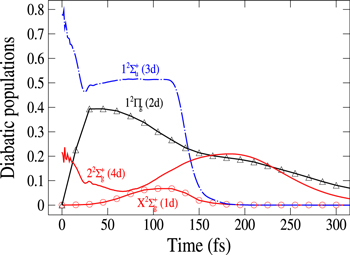
Figure 4. Time dependence of diabatic populations after excitation in the 3a state. States of  symmetry: solid line without symbols
 (1d), circle
  (4d). Line dots
  (3d). Triangle up
  (2d). For clarity, the populations in the 5d and 6d states, remaining weak, have been suppressed.
Download figure:
Standard image High-resolution imageFinally, we show in figure 5 the adiabatic populations as a function of time for initial excitations in the adiabatic states 3a (upper panel) and 2a (lower panel). The main dynamical features obtained above are still observed. In the upper panel, the dynamics starts in the adiabatic 3a state, which mainly corresponds to the diabatic  (3d). Here again, the rapid elongation of the interatomic distance Li-Li drives quickly the wavepacket to the conical intersection I1. Beyond this point, the state 3a has mainly a
  character and state 2a a
  character. As observed in the diabatic populations (figure 2) the passage through I1 is rather diabatic, the wavepacket dissociating, for the most part, in state 2a (
 ). As above the wavepackets are absorbed by the CAPs around 130 fs (2a) and beyond 200 fs (3a). The lower panel in figure 5 displays the flux redistribution for initial excitation in the 2a state. The inset shows the long-time redistribution. Compared with the upper panel, we observe that the adiabatic population in the initially populated level decreases more slowly, and here again, the time for reaching the I1 conical intersection is obviously longer, since the energies included in the wavepacket are weaker than for excitation in the 3a state. As before (figure 3) the wavepacket in state 3a is mostly trapped in this state beyond the conical intersection I1. The transfer to the 2a state in the long-time domain is seen in the structure displayed in the inset. Note that the 4a state is too high to be populated, the wavepacket remaining trapped in the lower 3a PES where it oscillates either in the basin of the
  state or the
  state.
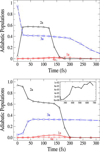
Figure 5. Upper panel: time dependence of adiabatic populations after excitation in the 3a state. Lower panel: time dependence of adiabatic populations after excitation in the 2a state. The inset in the lower panel shows the longer time evolution of the 2a state. For clarity, the populations in the 5a and 6a states, remaining weak, have been suppressed. The symbols on the curves correspond to the calculated adiabatic points.
Download figure:
Standard image High-resolution imageIn addition to the adiabatic populations in the different states, accessible parameters are the dissociation rates in the two asymptotic channels, namely the lower Li  Li+ asymptote or the upper Li
  Li+ asymptote. As already noted above, two states, 1a and 2a in the adiabatic basis or 1d and 3d in the diabatic basis, correlate with the lower asymptote and four states, 3a to 6a, or 2d and 4d to 6d, with the upper asymptote. In figure 6 the displayed time-dependent photofragment distributions represent the sum of the adiabatic populations associated to both asymptotes. The dynamics starts in the 3a state in the upper panel and in the 2a state in the lower panel. We observe that diabatic and adiabatic populations become virtually identical in the long-time domain, where the couplings do not affect the dissociation rates. As long as we are interested in an initial population in the 3a state, where the photoexcitation energies are high enough to avoid the trapping in the
  state (at least for a very large the part of the wavepacket), the rates are mostly governed by the short-time flux redistributions, before the wavepackets reach the CAPs. The transfers depend on the couplings in the Franck–Condon region and on the passage through the I1 conical intersection, the passage through I2 inducing only redistributions among the 4 states (3a-6a or 2d and 4d to 6d) which correlate with the same upper asymptote and thus, does not change the final rates. For an initial population in the 3a state, in a purely adiabatic limit, these rates would equal 0 for the lower Li
  channel and 1 for the upper Li
  channel. Deviations from this limit shed light on the strengths of the non-adiabatic couplings inducing redistribution of the photodissociation flux. We see here a strong deviation from this adiabatic picture since around 58% of the wavepacket dissociates in the lower asymptote.
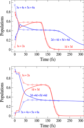
Figure 6. Time dependence of the sum of the adiabatic / diabatic populations which correlate with the  and
and  asymptotes of Li
 — Ne. Upper panel: after excitation in the 3a state. Lower panel: after excitation in the 2a state. Solid lines: sum of diabatic states. Dashed lines: sum of adiabatic states. The symbols on the curves correspond to the calculated adiabatic points. The sums 1a + 2a and 1d + 3d are associated to the lower
  asymptote, the other sums being associated to the upper
  asymptote.
Download figure:
Standard image High-resolution imageFor an initial population in the 2a state, the analysis is more complex. The flux redistribution and the absorption by the CAPs occuring in the long-time region (See the inset in figures 3 and 5) prevent to quantify accurately the final rates. The short-time evolution allows, solely, to find a lower limit for the dissociation rate in the lower asymptote and conversely an upper limit for the dissociation rate in the upper asymptote. Here, the adiabatic limit would predict 1 for the lower Li  Li+ channel and 0 for the upper Li
  Li+ channel. We see clearly, that whatever the transfers at long-time, the adiabatic picture is appropriate since, at least 68% of the final flux is in the lower asymptote.
4.2. Classical dynamics
The dynamics is initiated by a Frank-Condon transition from the ground state to one of the three adiabatic states (two in A' and one in A" symmetries) and coupled by dipole transition to the ground state of the Li2+Ne molecule. The initial conditions were obtained by sampling the three internal coordinates of the molecule from harmonic oscillator distribution function [44], which takes into account the ZPE motion in the electronic ground state. The assumption of harmonicity is in close agreement with the MCTDH analysis. The dynamics is then followed during 5 picoseconds by means of the TSH method, using the fewest switches algorithm [45]. For each adiabatic state, a swarm of 200 trajectories was run. A complete description of the method can be found in [44].
The dynamics of the A" states that correlates with the  state of Li2+ exhibits a relatively simple behavior. It is insensitive to the conical intersections identified by I1 and I2. The molecule is trapped in the potential well of the
  state of Li2+. We observe that 25% of the trajectories lead to the loss of the Ne atom, leaving a weakly vibrationally excited molecule Li2+. In the remaining 75%, the Ne atom is still bound after 5 ps. These different histories will eventually lead to radiative decay with an energy spectrum characteristic of the exit channel.
As described in the quantum calculations section, the dynamics of the 2 states that belong to the A' symmetry subgroup (2a and 3a according to the definition of section 2.2) is very different from the dynamics of the state in the A" symmetry, because the Ne atom couples together the  and
and  states of Li2+ to form the conical intersection I1 and the
  and
and  states of Li2+ to form the conical intersection I2. When the excitation takes place in the third adiabatic state of this symmetry (3a), the classical simulation is in quantitative agreement with the MCTDH simulation. We observe that 50% of the classical trajectories leads to complete atomization of the system with the formation of one Li(2s) atom, while 50% remains in an excited electronic state correlated with the Li
  asymptote. The proportions observed in figure 6 for MCTDH simulation are 58% and 42% respectively. One origin of the observed difference is in the diabatization procedure. Indeed, the diabatization shifts the 3a state by 0.06 eV in the Frank-Condon area. Though this is not much for the transition energy, the wavepacket reaches the intersection I1 with more kinetic energy so that the transfer toward the 2a PES is more likely. When the system remains in one of the excited electronic states correlated with the Li
  asymptote, most of the trajectories leads to the ejection of the Ne atom. In such a case, our diabatization procedure ensures that the diabatic and adiabatic states become identical. From the classical molecular dynamics, we observe that approximately 30% of the trajectories ends in the
  state of Li2+ and 20% in the
  state. The comparison with the diabatic population deduced from the MCTDH simulation after a propagation of 200 fs (figure 4) following excitation in the 3a state is rather consistent with these proportions (around 20% for each state). When the excitation takes place in the second adiabatic state of the A' symmetry (2a), as in the MCTDH calculation, the classical dynamics has a pronounced adiabatic character. Roughly 65% of the classical trajectories (compared to 68% in the quantum population) leads to complete dissociation with the formation of a Li(2s) atom. The remaining part is mainly concentrated in the
  state of Li2+ and a small fraction is left in the
  state. In these cases the probability to eject the Ne atom is comparable to that of keeping it bound to the molecule. Among the dissociative trajectories, approximately 5% dissociates between 1 and 5 ps after a transient stabilization on the
  state. The quantization of the dynamics apparently plays a minor role in the state populations. The coupling with the dissociative continuum of the
  state decreases the interference effects associated with the confinement in the potential well leading to the correct description of the populations with classical dynamics.
4.3. Photoexcitation cross-sections
The quantum photoexcitation cross-sections are calculated through a Fourier transformation of the autocorrelation function C(t) [57–59]:

Figure 7 (upper panel) displays the calculated photoexcitation cross-sections for transition from ground state to adiabatic 2a and 3a states. Also shown for comparison, are the cross-sections obtained in the classical approach. The latter were obtained by sampling the Wigner distribution associated to the vibrational motion on the ground state PES in the harmonic approximation. It provides us the distribution of transition energies from the ground state PES to the excited state PESs, and therefore the photoexcitation cross-sections in the Frank-Condon approximation [4, 43, 44]. The qualitative agreement between the calculated spectra is quite good. As discussed in an earlier study, the addition of a Ne atom leads to a spectral blue shift of the  −
−  transition which is, compared to the
  −
−  transition, shifted towards higher energies. The steepness of the 3a PES leads to a structureless broad band, with a small shoulder corresponding to the crossing of the PESs at the conical intersection I1. Moreover, as discussed above, the difference in the
  −
−  spectrum between the classical and the quantum results is an indication of the accuracy of our diabatization procedure, which shifts the 3a state by 0.06 eV in the Franck–Condon region.

Figure 7. Upper panel: quantum (solid lines) and classical (dashed lines) photoexcitation cross-sections for excitation in the adiabatic 2a and 3a states. Lower panel: zoom of the quantum cross-sections after excitation in the 2a state (solid line) and in the 2d state without couplings (dashed line). Dots: eigenenergies for the uncoupled 2d state. For sake of clarity the dots have been displayed twice.
Download figure:
Standard image High-resolution image
For excitation in the adiabatic 2a state, a great part of the wavepacket oscillates in the well of the binding PES, leading to recurrences in the autocorrelation function, responsible for vibrational resonances in the quantum absorption spectrum. The lineshapes resonances are a direct measure of the couplings strength. In order to shed light on the role of these couplings, we have carried out calculation of the photoexcitation spectrum for transition from the ground state to the diabatic 2d state (equivalent to the adiabatic 2a state in the Franck–Condon region), in canceling all the couplings. The results are displayed in the lower panel of figure 7, where we observe that the couplings lead to slightly more diffuse resonances which are shifted in energy. Finally, we have computed the eigenenergies corresponding to the uncoupled 2d state in diagonalizing the Hamiltonian using the Lanczos algorithm [11]. The eigenenergies reported in the lower panel of figure 7 confirm that the resonances observed in the spectrum are due to the vibrational structure of the 2d state.
5. Conclusion
The relaxation dynamics of the Li2+Ne trimer has been investigated as a prototype of the dynamics of a dimer weakly perturbed by an additional inert atom. Despite the weakness of the interaction, our study shows that the conical intersections I1 and I2 play an important role in the dissociation process. The conical intersection I1 originating from the  and
and  crossing of the bare Li2+ is even of paramount importance for the relaxation of the system, since it involves states correlated with different asymptotes.
Both quantum and classical simulations show that the dynamics takes place in two temporal stages. In the first one, the population flows quickly toward the Li  + Li+ + Ne dissociation channel. The duration of this stage is of the order of 20 fs for excitation in the third adiabatic state and is characterized by a dominantly diabatic character, for which the system is driven through the conical intersection. The duration of this stage is longer for the flatter PES of the second adiabatic state, i.e approximately 40 fs. In this case, the process is predominantly adiabatic, and associated to a smooth rotation of the π orbital in the molecular plane to form a
  orbital. The part of the population that does not lead to fast dissociation remains trapped in the well of the PES originating from the
  state of the bare Li2. The motion has a marked diabatic character in this case. During this second stage, two processes occur, according to the vibrational energy accumulated in the system. We observe indeed a competition between two processes: (i) the loss of the Ne atom, which hinders the Li2+ molecule to go, through the conical intersection, toward the Li
  +Li+ dissociation channel, (ii) the slow process associated to the recurrent exploration of the conical intersection by the vibrating molecule transiently trapped in the potential well of the PES correlated with the
  state of the bare Li2+. The characteristic time of the process is in the picosecond range and only a small fraction of the population follows this route.
Despite their conceptual differences, the classical and quantum simulations are in close agreement regarding the population dynamics and fragmentation pattern. The vibrational structure, which is clearly observable in the cross-section for excitation into the second electronic state, is apparently of limited significance for short pulse excitation like the one investigated here. The Rabi-like oscillations observed during the first few femtoseconds of the dynamics reflect mainly the coherent mixing of the diabatic states to build up the adiabatic states. They have apparently a negligible influence on the dissociation dynamics.
Acknowledgments
The Laboratoire de Physique des Lasers, Atomes et Molécules (PhLAM) is unité associée au CNRS, UMR 8523. All quantum calculations were carried out using the Heidelberg MCTDH package. The authors are grateful to all developers. This work was performed using the PhLAM High-Performance Computing linux Cluster (HPC) of Université Lille 1. The authors acknowledge the PhLAM laboratory and the CaPPA project (Chemical and Physical Properties of the Atmosphere), funded by the French National Research Agency (ANR) through the PIA (Programme dʼInvestissement dʼAvenir) under contract ANR-10-LABX-005 for financial contributions for the HPC. BP and MM are grateful to L Gonzalez and C Deroo, Laboratoire dʼOptique Atmosphérique of Université Lille 1, developers of the MGRAPH graphics software.