Abstract
Relativistic electron beam propagation through solid density plasma is a rich area for magnetic field dynamics. It is well known that Ohmic heating of the background plasma caused by the beam significantly affects magnetic field generation, primarily through changes in the resistivity. In particular, temperature changes in the background plasma leads to the generation of a magnetic field that acts to deflect relativistic electrons from the beam axis. This 'beam hollowing' field could have disastrous implications for the fast ignitor scheme.
In this paper, the effects of background heat flow on magnetic field generation are considered, first with a simple analytic investigation, and then with 1D Vlasov Fokker–Planck and classical transport simulations using a rigid beam for the fast electrons. It is shown that the thermal conduction of the background plasma acts to diffuse the temperature, reducing both the temperature gradients and the beam hollowing field. This gives rise to the re-emergence of a collimating magnetic field. The influence of the background heat flux is also investigated in the context of solids with imposed resistivity gradients, and is shown to significantly enhance the magnetic field present. More exotic transport effects, such as an enhanced Nernst velocity (due to non-local heat flux) and double peaked temperature profiles (due to distortion of the heating and heat-flow profiles by the magnetic field), are also reported.
Export citation and abstract BibTeX RIS

Content from this work may be used under the terms of the Creative Commons Attribution 3.0 licence. Any further distribution of this work must maintain attribution to the author(s) and the title of the work, journal citation and DOI.
1. Introduction
The success of the fast ignitor (FI) [1] approach to inertial confinement fusion (ICF) hinges on the ability to couple the energy of a short pulse high intensity laser to the dense fuel core via moderately relativistic electrons. The FI hotspot requires a temperature of 12 keV and a ρ RHS = 0.6 g cm−2 [2], where RHS is the hotspot radius and ρ is the fuel density. For a fuel density of 300 g cm−3, these values lead to limits on the energy contained in the fast electron beam to be E > 14 kJ, with the requirement that this energy must reach the fuel core in a time less than the expansion time of the hotspot, approximately 20 ps [3]. From energy deposition conditions [4], the electrons require an energy of approximately 1 MeV. For a hotspot radius RHS < 20 µm, this yields a current density of 5.5 × 10¹³ A cm−2, and a current of almost 1 GA. This current exceeds the Alfvén current limit [5] by five orders of magnitude, and fast electrons can only pass through the background plasma by drawing a nearly equal and opposite return current [6]. The electric field required to draw the return current decelerates the fast electrons [7], generates magnetic field structures inside the plasma [8, 9], and causes Ohmic heating of the background plasma. A full understanding of the evolution of these fields generated over 20 ps duration is therefore crucial for the success of the FI scheme, and is of interest to current and future laser–solid experiments.
The fast electrons must travel from the critical density region, where the high intensity short pulse laser deposits some of its energy into these electrons, to the high density core. This represents a 105 change in background electron number density, from approximately 1021 cm−3 (critical density) to 1026 cm−3 (dense fuel core). Such a range of conditions and associated time scales makes the FI scheme a particularly challenging problem to simulate. Kinetic simulations, such as explicit Particle in Cell (PIC), are adept at modelling the laser deposition and fast electron transport near critical density. However, these methods become computationally expensive deeper into the target. The requirement to resolve the background electron plasma period, and often the background Debye length, limits simulations of solid density targets to sub-picosecond durations. Hybrid simulations [10–12] offer a solution to this issue by melding the kinetic description of the fast electrons with a reduced description of the background plasma. Despite the success in modelling picosecond laser–solid experiments [9], many classical transport effects are often neglected in the background plasma. These include thermal conduction in the background plasma, Nernst advection [13], and other magnetic field dynamics [14], which may become important over tens of picoseconds. These effects could therefore be important for the evolution of the fast electron beam over picosecond time scales.
In this paper, a simple analytical model is developed for assessing when thermal conduction effects in the background plasma is likely to be important. This model is tested by using a rigid beam fast current coupled into the Vlasov Fokker–Planck (VFP) code IMPACT [15]. These simulations are corroborated by using the same setup in the classical transport code CTC [16]. These 1D simulations show that in the case of a fully ionized carbon plasma with initial temperature 100 eV, thermal conduction effects can cause significant spreading of the temperature profile in the background plasma over picosecond time scales for solid and near solid densities. The temperature spreading significantly affects the magnetic field generation over picosecond time scales, and acts to suppress the magnetic field generation due to temperature gradients in the background plasma (the so called 'beam hollowing' field [17]). These effects are then considered in the context of engineered resistivity gradients [12, 18, 19].
2. Beam hollowing
The dominant mechanisms for magnetic field generation familiar to students of fast electron transport are the resistive generation of field and the 'beam hollowing' field generated by resistivity gradients. Consider the reduced Ohm's law electric field E = ηjr, where η is the resistivity and jr is the return current density. Substitution into Faraday's law and using Ampere's law (for the total current density jf + jr), yields

where jf is the fast electron current density, and resistive diffusion effects of the magnetic field have been omitted. The first term on the right-hand side represents resistive generation of the magnetic field. Consider the situation where a fast current directed along the −x-axis (representing fast electrons propagating along the x-axis), with a Gaussian profile along the y-axis of the form jf = j0 exp(−ay2) with a > 0 and j0 < 0. The magnetic field generated is such that it acts to pinch the fast electron beam. This effect has aroused a great deal of interest in the community as a means of collimating the fast electron beam [8]. The second term on the right-hand side of (1) acts to deflect electrons towards regions of higher resistivity. For resistivities that decreases with increasing temperature, and a background plasma that Ohmically heats in response to the influx of fast electrons, the magnetic field generated acts to deflect the fast electrons away from the centre of the beam. That is, the magnetic field generated acts to hollow the fast electron beam. This mechanism was used to explain the annular formations of fast electrons observed at the back of mylar targets [9].
One can consider the competition between these two magnetic field generation mechanisms by considering a background temperature profile Ohmically heating

where Te is the background electron temperature (in units of energy), ne is the background electron number density (assumed homogeneous throughout this work) and cg = 3/2 for an ideal gas. Here η is taken to be the Spitzer resistivity [20]

where Te0 is the initial background electron temperature and η0 = α⊥me/τ0nee2 is the initial background resistivity. Here me is the electron mass, e is the electron charge, τ0 is the initial background electron–ion Braginskii collision time [21] and α⊥ is the Braginskii dimensionless resistivity coefficient with the correction by Epperlein [22, 23]. In using the Spitzer resistivity, material effects [24] are neglected in this work. The fits of Davies et al [25] to the material resistivities of Milchberg et al [26] and Downer et al [27] suggests that, for a plastic-like or carbon target, a starting temperature of 100 eV is sufficient to ensure that the Spitzer resistivity overestimates the actual resistivity by no more than 25%, and this disagreement decreases as the temperature increases. Proceeding with the Spitzer resistivity, (2) can be integrated to yield

and (1) can be integrated to yield

In the region y > 0, consideration of the fast electron trajectories along the x-direction lead to the conclusion that a Bz < 0 will collimate the fast electrons. In the limit that the first two terms in the square parentheses in (5) dominate, the time for the field in this region to change sign can be estimated as

where
 , vf is the fast electron velocity, c is the speed of light in vacuum, n23 = ne/1023 cm−3, TkeV,0 = Te0/1 keV, ln Λ is the Coulomb logarithm and Z is the average ionization. Taking
 (the peak magnetic field growth rate will occur near where ∂yjf(y) peaks, and not at the peak of jf(y)), and also Z ln Λ = 12, n23 = 1, nf/ne = 0.01, vf/c ≈ 1, the inequality in (6) yields a time of approximately 250 fs. For n23 = 5, and ne/nf = 0.002, this time is now 1250 fs. Note that these are estimates for when the magnetic field changes sign from a collimating field to a hollowing field. It does not necessarily mean that the beam will actually hollow. Estimating if and when a beam will hollow depends on the full form of (5), as well as a consideration of the Larmor radii of the beam electrons moving in the hollowing field. Furthermore, while the beam hollowing field in the n23 = 5, ne/nf = 0.002 case takes five times longer to develop than in the n23 = 1, ne/nf = 0.01, the magnitude of the fields will be larger as a result of the presence of ne in (5). Note that ne is also hidden in Te. In the limit of Te ≫ Te0, the magnitude of the magnetic field is expected to scale as
 .
.
3. Theoretical estimates of thermal conduction
The discussion in the previous section neglects the effects of thermal conduction in the background plasma. As the magnetic field has been shown to be strongly dependent on the temperature profile in the background plasma (see (5)), one would expect that thermal conduction could become important as the background plasma heats, and the mean free paths of the background electrons increase. An estimate for the time when thermal conduction effects are likely to be important can be found by comparing the divergence of the diffusive heat flow

to the Ohmic heating rate
 . Here
 is the unit vector along the y-axis, and κ⊥ is the dimensionless thermal conductivity coefficient given in [21–23]. By making use of

which arises from taking the y-derivative of (4), it can be shown that at y = 0

Note that y = 0 is chosen as it is the position where (7) peaks. In the limit of strong heating, whereby it is meant that the temperature rise by Ohmic heating is much greater than the initial temperature, one finds

where
 is the full width at half maximum of the fast electron beam. Ratio (10) is expected to depend only weakly on Z given that
 varies between 1.27 → 2 for Z = 1 → ∞, when classical transport theory is valid [22, 23]. By setting the left-hand side of (10) equal to unity, one can find the time t = ttc for thermal conduction to become significant. For a system with ne/nf = 0.01, Te0 = 100 eV and FWHM = 10 µm, (10) suggests that thermal conduction will begin to significantly contribute to the temperature evolution after approximately 500 fs. The time ttc scales linearly with FWHM, and inversely proportional to the beam to background ratio nf/ne. The limit of strong heating is valid after approximately 10 fs at y = 0 for Te0 = 100 eV, ne = 1023 cm−3, Z ln Λ = 12 and nf/ne = 0.01. This limit may not be valid in the wings. However, these wing effects are not expected to be important as the key region of competition between the Ohmic heating rate and diffusive heat flow will be near the centre of the beam.
4. Simulation details
To progress this investigation further, a rigid beam fast current is coupled into the VFP code IMPACT [15]. IMPACT is suited to describing full collisional transport, including magnetic fields and non-local effects, and does not assume a Maxwellian background electron distribution function. IMPACT solves the VFP equation by making use of an expansion of the distribution function in velocity space anisotropy f = f0 + f1 · v/v + ···. The so-called Cartesian tensor expansion [28] is curtailed after the second term, such that anisotropic pressure and higher order anisotropic terms are neglected. This is justified by the fact that electron–ion collisions act to isotropize the distribution function in velocity space. This so-called diffusion approximation has been shown to be valid even when f0 ∼ |f1| [29]. Furthermore, the following results have been tested against modified version of IMPACT with the
 term retained, and no significant changes to the results are observed. IMPACT also includes hydrodynamic effects via a fluid model. Note that ion acoustic turbulence, thought to lead to an anomalous resistivity [30], are neglected in this work.
The geometry used in the simulations is identical to that assumed in sections 2 and 3: a rigid fast current with density 4.8 × 10¹² A cm−2 is directed along the −x-axis. This fast current is included in the initial conditions of IMPACT and draws a collisional, neutralizing return current in the background plasma. The fast current has a Gaussian profile of the fast current along the y-axis giving rise to magnetic field growth along the z-axis. No spatial gradients are considered along the x-axis. The y-axis has periodic boundary conditions imposed, and a spatial extent of 8 × FWHM. The y-range [−4FWHM : 4FWHM] has been chosen to ease discussion, and most of the plots in the following sections only show the range [−2FWHM : 2FWHM], where most of the interesting physics occurs. A grid size of 16 × FWHM and the use of open boundary conditions has been tested, with negligible difference between the results. Details of the parameters used for the main simulations presented in this paper can be found in table 1. Note that the simulation results have been tested against a range of simulations with better y- and v-grid resolutions, as well as simulations using five times smaller time-steps. Little difference between the results was observed.
Table 1. Table of simulations parameters. Here Te0,keV is the background starting temperature in keV, n23 is the initial background number density in units of 1023 cm−3, FWHMµm is the FWHM of the fast electron current density in microns, Δyµm is the y-resolution in microns, Δtfs is the time-step in femtoseconds,
 is the velocity space resolution in units of µm ps−1, nv is the number of velocity space cells, and
 .
.
| Section | Simulations parameters | |||||||
|---|---|---|---|---|---|---|---|---|
| Z(y) | Te0,keV | n23 | FWHMµm | Δyµm | Δtfs |
|
nv | |
| 10 | 0.4 | |||||||
| 5 | 6 | 0.1 | 50 | 2.0 | 0.21 | 2.1 | 80 | |
| 6 | 6 | 0.1 | 5.0 | 10 | 0.4 | 0.04 | 2.1 | 80 |
| 7 | 2.67 for |y| > FWHM | 0.1 | 5.0 | 10 | 0.4 | 0.04 | 2.1 | 80 |
| g(y) for |y| < FWHM | ||||||||
The results seen in the VFP simulations are corroborated by performing the same simulations with the classical transport code CTC [16, 31]. CTC contains full Braginskii transport as well as hydrodynamic motion. It has the useful feature of being able to turn particular transport effects on/off, a feature absent in IMPACT, and is thus invaluable in the current study. The simulation parameters are the same as those listed in table 1, with the exception that velocity space parameters are not relevant to the CTC case.
5. Near solid density fully ionized carbon
This section considers VFP simulations of a homogeneous background plasma with ne0 = 1023 cm−3 and Z = 6, and a peak fast electron current density 4.8 × 10¹² A cm−2. In figure 1 the Bz and Te profiles are shown for a FWHM = 10 µm beam at 0.5 ps and 1.5 ps. The 0.5 ps profiles compare very well to the estimates presented in the section 2. However, the 1.5 ps profiles differ significantly from those estimates. In particular, the Te profile is broader and lower than the estimated profile. This results in smaller resistivity gradients in (1). The fluid theory without thermal conduction clearly predicts a beam-hollowing field either side of the centre of beam at y = 0 µm at this time, while the simulation results show a collimating field. As the importance of thermal conduction depends on the size of temperature gradients in the system, the results of a broader fast electron profile would provide a useful comparison. Figure 2 provides just such a comparison, showing the profiles of a FWHM = 50 µm beam at 1.5 ps. These show good agreement with the estimated profiles at this time, supporting the theory that the phenomenon shown in figure 2 is due to thermal conduction.
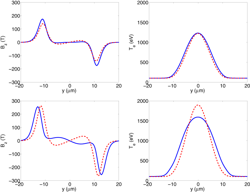
Figure 1. Left: Magnetic field at 0.5 ps (top) and 1.5 ps (bottom) as predicted by the VFP-rigid beam code (solid blue) and by the estimate provided in (5) (dashed red) for FWHM = 10 µm. Right: Temperature profile at 0.5 ps (top) and 1.5 ps (bottom) as predicted by the VFP-rigid beam code (solid blue) and by the estimate provided in (4) (dashed red) for FWHM = 10 µm.
Download figure:
Standard image High-resolution image
Figure 2. Magnetic field (left) and temperature profile (right) at 1.5 ps as predicted by the VFP-rigid beam code (solid blue) and by the estimates provided in (5) and (4) (dashed red) for FWHM = 50 µm.
Download figure:
Standard image High-resolution imageTo confirm that the phenomenon arises due to effects of heat flow broadening the temperature distribution, the contributions of ∇ · q and Ohmic heating to the total heating rate at 0.5 ps for the FWHM = 10 µm are shown on the left of figure 3. The divergence of the heat flow (∂yqy in this geometry) makes a significant contribution to the overall heating rate, removing thermal energy from the centre of the beam and depositing it in the wings. This contribution has been observed to be negligible in the case of the FWHM = 50 µm at 0.5 ps.

Figure 3. Left: Heating rate profile for the FWHM = 10 µm case at 0.5 ps. Thermal conduction effects (dotted–dashed blue) act to spread the temperature, leading to a broader total heating profile (dashed black). Right: Contribution of ηjrx to the x-component of the electric field for the FWHM = 10 µm (solid blue) and FWHM = 50 µm (dashed red) cases at 0.5 ps. The y-values have been normalized to FWHM in each case. Notice the re-emergence of a centre-peaked electric field in the FWHM = 10 µm which is absent in the FWHM = 50 µm at this time.
Download figure:
Standard image High-resolution image5.1. Re-emergence of a centre-peaked electric field
In the right hand plot of figure 3, the contribution of ηjr to the x-component of the electric field is shown for both FWHM = 10 µm and FWHM = 50 µm. The FWHM = 50 µm field has been 'hollowed' by the rising temperature at the centre of the beam. The FWHM = 10 µm also shows this hollowing, but also exhibits a re-emergence of a centre-peaked electric field. It is this re-emergence that gives rise to the beam-collimating field generation shown in figure 1, which allows the beam hollowing field to be overcome. Note that in calculating the transport terms, such as ηjr, the simulation distribution function was used. That is to say, a Maxwellian distribution was not assumed. A prescription for doing this is given in the appendix.
5.2. Comparison with CTC
The above results can be tested against the classical transport code CTC [16], which (as stated above) has the advantage that one may turn off heat-flow effects in the energy equation, a function not possible in IMPACT. This allows further confirmation of the action of heat flow in causing the re-emergence of a collimating field. Figure 4 shows the temperature and magnetic field profiles at 1.5 ps. Notice the presence of the beam hollowing field in the simulations without heat flow, compared to a beam-collimating field present in the simulation with heat flow. The CTC run with heat flow still predicts the presence of the beam hollowing field near the y = 10 µm mark, while the VFP simulation predicts beam collimating in this region. This is due to suprathermal electrons streaming from warmer regions, preheating the region in and around y = 10 µm in the VFP case. These electrons are of course absent in the CTC case. This leads to a smoother temperature profile in the VFP case, as compared to the CTC case, and thus a reduced rate of magnetic field generation due to resistivity gradients. This is evidenced in the temperature profiles for the VFP and CTC (with heat flow) at 1.5 ps.

Figure 4. Left: Comparison of magnetic field profiles predicted by IMPACT (solid blue), CTC with (dashed red) and without (dotted–dashed black) y heat flow qy at 1.5 ps. Right: Comparison of the temperature profiles predicted by IMPACT (solid blue), CTC with (dashed red) and without (dotted–dashed black) y heat flow qy at 1.5 ps. The difference between the IMPACT and CTC with heat-flow simulations is due to the lack of a flux limiter in the latter.
Download figure:
Standard image High-resolution image5.3. Parameter scan
It would be useful to quantify the effect of thermal conduction in a more precise manner than that presented in section 3. In that section, simple fluid estimates were used to estimate the time ttc when the divergence of the diffusive heat flow becomes significant compared to the Ohmic heating rate. However, as the temperature is given by the time-integrated energy equation, there will be a delay between the thermal conduction being a significant contribution to the energy equation, and the effects of thermal conduction actually becoming apparent on the temperature profile. As the thermal conduction acts to spread the temperature profile, an obvious improvement would be to consider the evolution of the dimensionless measure

as defined by Epperlein [32]. Here 〈Te〉 is the spatial average of the temperature along the y-direction. This term can be considered as a measure of the spreading of the temperature. Higher values of σrms are expected for sharply peaked temperature profiles, and lower values are expected for a broad temperature profile close to the average temperature. The left plot in figure 5 shows the time evolution of σrms for FWHM = [10, 20, 30, 40, 50] µm, as measured in the VFP simulations. Consider the 50 µm curve up to a time of 2 ps, when heat flow effects are not important. While σrms levels off as a result of the Ohmic heating rate saturating, it does not decrease. Now considering the 10 µm case; σrms peaks and starts decreasing at approximately 1.2 ps. This is the effect of heat flow becoming apparent on the temperature distribution.
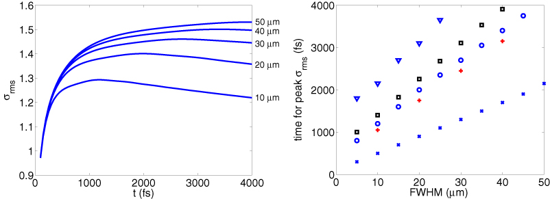
Figure 5. Left: Evolution of σrms (11) over 4 ps for a range the FWHM 10, 20, 30, 40 and 50 µm (labelled on the right-hand side of the plot). Right: Parameter scan of the time for σrms to peak. This gives an indication as to when thermal conduction effects are beginning to have an impact on the temperature distribution. C (Z = 6) simulations are given by ○(nf/ne = 0.01), ×(nf/ne = 0.007), ▿ (nf/ne = 0.014). Al (Z = 13, nf/ne = 0.01) □. CH Z = 2.67, nf/ne = 0.01) +.
Download figure:
Standard image High-resolution imageThe right plot in figure 5 shows a scan of the time for the temperature spreading function σrms to peak versus FWHM for a range of background materials (C, CH2, Al) and a range of beam to background ratios, with all other initial conditions kept the same as above. It is useful to compare the characteristics of these lines to the simple estimates given in section 3. To recall, in section 3 it was shown that the time ttc for thermal conduction to become a significant contribution to the energy dynamics of the system had the form

where the constant of proportionality varies between 0.787 and 0.5 for low to high Z plasmas. On comparing (12) to the plots in figure 5, one notices the weak dependence on Z, and also the linear relationship between the time and the FWHM of the beam. The relationship between the gradient of the lines and the beam to background ratio also remains linear to within 15%. Finally, a good rule of thumb seems to be that the time for thermal conduction to start having a significant impact on the temperature profile is approximately 2ttc, that is

where k(Z) = [0.5 : 0.787], tfs is the time in femtoseconds, FWHMµm is the full width half maximum of the beam in microns and vf is the fast electron speed.
5.4. Exotic transport effects
It is interesting to consider more exotic transport effects that arise in the VFP simulations. One such effect is the Nernst effect, that is magnetic field is being advected down temperature gradients. Nernst advection arises, essentially, because the magnetic field is 'frozen in flow' to heat flux carrying electrons [13]. Consider figure 1. The peak magnetic field in the region y = 12 to 14 µm has moved a distance of 1.5 µm by 1.5 ps compared to its profile at 0.5 ps. Thus, a corresponding magnetic field 'velocity' of approximately 1.5 µm ps−1 is observed. The Nernst advection is a good candidate for this motion. The advection equation

where

can be found by considering the contribution of the thermoelectric effect to the induction equation [13]. Here, vN is the Nernst velocity, ωg is the electron gyrofrequency and β∧ is the thermoelectric coefficient in the direction perpendicular to both the magnetic field and the temperature gradient. Using the classical transport value for β∧ [22] and the temperature profiles from the simulation, vN can be easily calculated. Its profile is shown in the left plot of figure 6. Averaging the vN in the region y = 12 to 14 µm between the times 0.5 and 1.5 ps yields a value of vNy = 0.04 µm ps−1, an order of magnitude lower than predicted by the simulations. The reason for the discrepancy is due to the non-local flux of background hot electrons from the hot centre of the system to the cool wings. These hot electrons act to perturb the classical transport coefficients from the values predicted by a Maxwellian distribution. The actual Nernst velocity profile in the system is shown in blue in figure 6. The average Nernst adection speed in the region y = 12 to 14 µm between the times 0.5 and 1.5 ps is now vNy = 1.4 µm ps−1, in good agreement with the movement of the magnetic field observed. Note a prescription for how to calculate the Nernst advection speed for a non-Maxwellian electrons distribution function is given in the appendix.
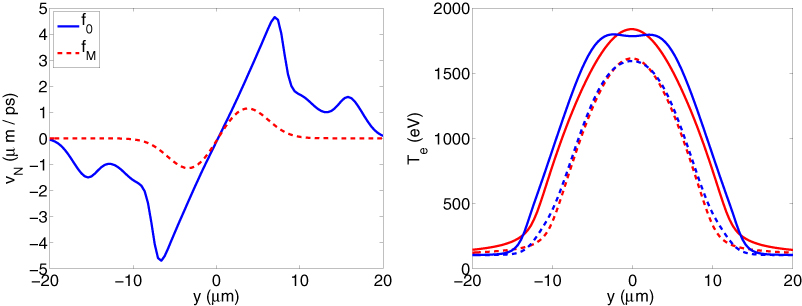
Figure 6. Left: Nernst velocity for the distribution function predicted by VFP simulation (labelled f0) and by a Maxwellian at the density and temperature predicted by the VFP simulation (labelled fM). Right: Temperature profiles at 1.5 ps (dashed) and 3 ps (solid) for VFP simulations with (blue) and without (red) the effects of magnetization included.
Download figure:
Standard image High-resolution imageAnother interesting transport phenomenon that has been uncovered by this work is the presence of a two-peaked temperature distribution, shown in figure 6. This phenomenon is inextricably linked to the magnetization of the background plasma. This is evidenced by the red curves in the right plot in figure 6, which show the temperature evolution when the VFP simulations are run with the effects of magnetic field in the background plasma turned off. To see why this two-peaked temperature distribution develops, consider the plot of the Hall parameter ωgτth (that is the electron gyrofrequency multiplied by the Braginskii electron–ion collision time) shown in figure 7. The Hall parameter is a useful measure of the degree of magnetization in a plasma. Notice that the there are two peaks. At y ≈ ±12 µm there is a peak in ωgτth due to the peak of the magnetic field being at this point (see figure 1). At y ≈ ±3 µm there is a larger peak ωgτth due to the re-emerged collimating magnetic field at this point, and also due to the temperature profile that has been spread by thermal conduction. Hall parameters of ωgτth ∼ 0.3 are significant to the heat flow as the β∧ coefficient peaks and the κ⊥ coefficient has fallen by a factor of 5 from its zero field value. The effect that magnetization has on the background plasma heating profiles can be seen by considering the heating rates predicted with and without magnetic field, shown in figure 7 That is, data from the full VFP simulation is used to predict the heat profiles if magnetic field were instantaneously turned off. Several effects occur. Firstly, the Ohmic heating profile is enhanced near the y ≈ ±3 µm due the increased resistivity (reduced mobility) of those current carrying electrons as a result of the magnetic field. Secondly, the Ettingshausen effect (β∧ heat flow) acts to divert current carrying electrons from the centre of the beam to y ≈ ±3 µm. These electrons then deposit their energy in that region. Finally, the diffusive heat flow (κ⊥) carrying electrons have their mobility reduced by the magnetic field, causing them to deposit their energy near the peaks of the magnetic field. This results in a higher heating rate profile at y ≈ ±3 µm for the case when magnetization is taken into account. This effect saturates after approximately 2.5 ps as the Ohmic heating rates reduce, the β∧ coefficient decreases for higher magnetizations, and the temperature gradients reduce in the region around y ≈ ±3 µm.

Figure 7. Left: Plot of magnetization at 1.5 ps (solid blue) and 3 ps (dashed red). Right: Difference between heating rate with and without magnetic field included in the calculation. Solid red represents contribution of η jrx, dashed blue the divergence of the Ettingshausen (β∧) heat flow, dashed green the divergence of the diffusive (κ⊥) heat flow, and dotted–dashed black the sum of these.
Download figure:
Standard image High-resolution imageFinally, IMPACT's hydrodynamic package allows the effects of the bulk motion of the background plasma to be turned on and off. Hydrodynamic motion has been shown to lead to significant cavitation of the background plasma [33], which could further enhance the suppression of the beam hollowing field through P dV cooling [34]. For the simulation parameters used in this work, heat-flow effects are far more significant than hydrodynamic effects in modifying the temperature and magnetic field profiles. Compared to a simulation with hydrodynamic motion included, a simulation with hydrodynamic effects neglected differs by no more than 2% in temperature and magnetic field profiles over 3 ps.
6. Solid density fully ionized carbon
The results presented in section 5.2 show that the CTC and IMPACT simulation results agree reasonably well. In this section, CTC is used to investigate the effect of transverse heat flow on the magnetic field dynamics in solid density targets, ne0 = 5 × 1023 cm−3, Z = 6. Again the peak fast electron current density is 4.8 × 10¹² A cm−2. Figure 8 shows the magnetic field profiles predicted over 10 ps for the case with qy = 0 (left) and qy ≠ 0 (right). After 10 ps in the qy = 0 case, a hollowing magnetic field of magnitude 300 T has developed in the region around y = ±7 µm. This hollowing magnetic field, with a spatial extent of approximately 5 µm is significant enough to deflect MeV fast electrons, travelling initially parallel to the x-axis, through an angle of 45° away from the centre of the beam. This will cause significant distortion to the fast electron beam. In the simulation with y heat flow, the 300 T hollowing field is replaced by ∼250 T collimating field. By considering fast electrons travelling in this field with a divergence half angle ϑ1/2, this field is significant enough to deflect 850 keV fast electrons through an angle of 45° towards the beam axis, and hence 'collimate' the beam.
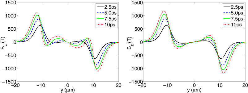
Figure 8. Plots of the magnetic field profile over 10 ps for CTC simulations with (left) and without (right) heat flow along the y-direction for solid density Z = 6 simulations. Note the presence of a ∼300 T hollowing field at y ≈ ±5 µm in the simulation without heat flow (left) at 10 ps, in contrast to the ∼250 T collimating field at y ≈ ±5 µm in the simulation with heat flow (right) at 10 ps.
Download figure:
Standard image High-resolution image7. Target engineering
In this section, a similar set up to that used by Robinson et al [12] is considered. Robinson et al considered an array of carbon guiding channels embedded within a plastic structure. The resistivity gradients at the boundary between the two materials generates a magnetic field through (1) which acts to reinforce the collimating field generated by the curl of the fast current. Robinson et al simulated the effect of this 'switchyard' structure on the propagation of fast electrons in 2D hybrid code simulations that did not include the effects of thermal conduction in the background plasma. In this section, thermal conduction effects on these target engineered magnetic fields is considered using CTC in a similar setup to that considered by Robinson et al. A FWHM = 10 µm beam is considered propagating through a homogeneous background plasma with density ne = 5 × 1023 cm−3, and an average ionization profile give by
which produces a smooth transition between a carbon plasma (Z = 6) at the centre of the system (y = 0), and a plastic-like material (Z = 2.67) at a distance FWHM from the centre. This Z-profile is modelled on and produces a similar Z-profile scale-length to those given by Robinson et al in [12, 19]. The peak fast electron current density is 4.8 × 10¹² A cm−2. The magnetic field profiles over 10 ps for the cases with and without heat flow in background plasma are give in figure 9. The case without thermal conduction in the background plasma (left plot) shows ∼0 T magnetic field in the region −5 µm < y < 5 µm, whereas the case with thermal conduction (right plot) shows a peak 400 T collimating magnetic field in that region. By considering fast electrons travelling in this field with an angle ϑ1/2 between the electron velocity vector and the x-axis, a field of spatial extent 5 µm is sufficient to collimate fast electrons with momenta p < 5 × 10⁻⁶eBz/(1 − cos ϑ1/2). Taking Bz = 400 T, a value ϑ1/2 = 45° leads to the collimation of fast electrons with energies <1.6 MeV, and a value ϑ1/2 = 60° leads to the collimation of fast electrons with energies <0.8 MeV. While these figures are rather approximate, and a realistic collimation criterion should take into account the magnetic field profile along the x-axis, these estimates suggest that hybrid simulations without thermal conduction in the background plasma could be significantly underestimating the collimation effects on fast electrons.

Figure 9. Plots of the magnetic field profile over 10 ps for CTC simulations with (left) and without (right) heat flow along the y-direction for solid density with Z gradients imposed. The Z profile used is given in table 1. The simulation with heat flow (right) exhibits a ∼400 T collimating field at y ≈ ±5 µm at 10 ps, in contrast the simulation without heat flow (left), which has no magnetic field in this region at that time.
Download figure:
Standard image High-resolution image
8. Discussion
The main result of this work is the influence that thermal conduction in the background plasma has on the magnetic field dynamics. The magnetic fields generated are expected to be able to significantly affect the trajectory of fast electrons. This work has focused on situations relevant to the FI scheme. The implications of this work for this scheme are clear: thermal conduction effects could help achieve a collimated fast electron beam in near solid and solid density regions of the plasma, and thus increase the coupling of fast electron energy to the core. The beam hollowing field investigated by Davies et al [17] has been shown to be mitigated and reversed by the thermal conduction spreading of the background plasma over picosecond time scales. Without these effects, beam hollowing could have disastrous implications for the feasibility of the FI scheme.
While the focus has been on FI relevant scenarios, it is interesting to consider the implication of this work for current and future laser–solid experiments. The useful rule of thumb for calculating when thermal conduction is likely to be important (13) can be transformed to the more practical form

where I20 is the laser intensity in units of 1020 W cm−2, ηL is the conversion efficiency of laser energy into fast electron energy, and εMeV is the average fast electron energy in units of MeV. Note that (16) does not take into account the coupling of the fast electron energy to the target. Fast electrons will slow down and spread as they propagate through the target, reducing the background heating and also the thermal conduction effects.
Equation (16) suggests that even for current high intensity lasers (I20 ≈ 1, with an efficiency typically ∼0.3), a reasonable FWHMµm = 5, the time for thermal conduction to become important will be on the order of a picosecond. This is near the limit of current laser pulse durations. An exception to this is the experiment conducted by Perez et al [35], whereby a cylindrical compression of a plastic foam is followed by a 10 ps, I20 = 0.05 heating laser in the transverse direction to the compression. For the case of the low density foam (ρ = 0.1 g cm−3) they observed a collimated fast beam for longer compression-heating delays. The reduced Ohmic heating at the peak of the shock (as a result of the higher density, and thus higher heat capacity there compared to the rest of the foam) resulted in resistivity generated in a favourable manner for collimation. From data given in [36] and (16), the effect of thermal conduction is likely to be important in the range 0.5 ps to 3 ps (depending on the density considered), well within the 10 ps pulse duration. While the hybrid code used to model the experiment did include the effects of thermal conduction in the background, these effects are not mentioned in [36] and warrant further investigation.
A repeat of the Norreys et al experiment [9] with a pulse duration of 4 ps may be a possible avenue for near-term future experiments. These experiments observed the annular formation of the fast electrons at the back of the mylar targets for the higher intensity experiments (3 × 10¹⁹ W cm−2). Equation (16) predicts a time of approximately 3 ps for thermal conduction effects to appear. The findings of the paper suggest that by extending the pulse duration, the annular electron beams inferred by Norreys et al [9] would disappear as a result of the phenomena discussed in this work, and would make an interesting experimental campaign.
8.1. Relevance to laser–solid experiments
It should be emphasised that the work presented in this paper relates to 1D rigid-beam descriptions of fast electrons propagating through a background plasma where the VFP formalism is valid. Laser–solid experiments can differ greatly from this reduced picture. Laser–solid experiments typically have starting temperatures of a fraction of an electron-volt and exhibit material-dependent phenomena, such as those observed in [24, 26]. These 'material effects' will strongly influence the resistivity on sub-picosecond time-scales in laser–solid experiments, and thus influence the magnetic field growth at these times. However, the background plasma will inevitably heat, due to the collisional return current it provides, and the effects of thermal conduction will increase in importance. The effects discussed in this paper will then play a role in the magnetic field dynamics. The impact of neglecting these 'material effects' on the simulations presented here can be estimated by comparing the material resistivity-fits provided in [17] to the Spitzer resistivity. For a carbon and a plastic-type material, the Spitzer resistivity is expected to overestimate the material value by approximately 15% to 25% at 100 eV, and by 5% to 10% at 200 eV. While these values are approximate, they suggest that the neglect of material effects is reasonable for a starting temperature of 100 eV or greater.
Ionization effects in the main simulation results presented in this paper are expected to be small. The average ionization of carbon plasma with ne0 = 1023 cm−3 at T = 100 eV is Z ≈ 4.8, and Z > 5.5 for T > 200 eV based on calculations with the non-LTE code ALICE II [38]. Thus, the approximation of a fully and homogeneously ionized carbon plasma is reasonable for these starting conditions. This is of course not true in laser–solid interactions. Picture a fast electron beam propagating through a lowly ionized carbon plasma. Qualitatively speaking, the Z-profile of the background plasma will become peaked on the beam axis, as this region draws the largest collisional return current and heats up quicker. With the temperature of the background plasma gradually rising, the situation starts to look reminiscent of the simulations presented in section 7. In reality the exact situation will depend on the exact values of the width of the beam and the width and scale of the Z-profile.
Laser–solid interactions also do not produce perfectly Gaussian fast electron profiles. In particular, the fast electron beam may break-up through the filamentation instability [39]. However, the work presented here may still be of relevance even in a completely filamented beam. Noting the linear relationship between the beam FWHM and the time for thermal conduction effects to become significant (see (13)), a fast electron filament with a width of a micron may be influenced by thermal conduction effects over 100 fs. While thermal conduction effects will not help guide the filament back to the beam axis (to the benefit of the FI scheme), it may help determine the size of the individual filaments. Work on characterizing the effect of thermal conduction on micron-scale electron beam filaments is ongoing.
A characteristic of fast electrons generated by laser–solid interactions is the large angular spread they posses as they enter the solid. Experimentally, a range of divergence half-angles have been measured, from 20° to 50° [40, 41]. When comparing the 1D simulations presented here to experimental results, care must be taken to account for the reduced fast current in the direction normal to the target, as a result of this spreading. For homogeneous targets, the effects discussed in this paper are most relevant near to the laser–solid interaction region, where the fast electron induced temperature gradients are large. As the electrons enter the target, their angular spread reduces the temperature gradients induced in the background plasma and thus reduces the diffusive heat flow. However, the FI scheme relies on the ability to guide a collimated beam of fast electrons through solid density regions. Whether the collimation is induced by resistivity gradients or otherwise, the 1D effects discussed in this paper may go someway to describing the salient features of such a situation. The effect of thermal conduction on 2D beam–plasma simulations will be the topic of a future publication.
9. Conclusion
This work shows that background heat flow can play a significant role in determining the electric and magnetic fields in a beam–plasma system, for solid and near solid densities. A simple model for when these effects are likely to influence the temperature profiles has been developed. The effects have been verified with 1D VFP simulations including a rigid fast electron beam, and the results corroborated with 1D classical transport simulations. The background heat flow is observed to spread the temperature profile such that 'beam hollowing' [17] fields are overcome, over picosecond time scales. The re-emergence of a collimating central field may be important in the fast ignitor scheme, where the establishment of collimating fields is crucial in guiding fast electrons to the fuel core. An approximate rule of thumb for calculating when these effects become important is given in (13), and shows that this time scales linearly with the beam FWHM and is inversely proportional to the beam to background ratio. In other words, tighter beams will create sharper temperature gradients, and will give rise to thermal conduction effects occurring sooner. Additionally, smaller beam to background ratios reflect the larger heat capacity of the background plasma and also smaller fast electron current density, both of which reduce the Ohmic heating rates, and thus extend the time for thermal conduction to become significant. The effects of thermal conduction have been considered in the context of engineered targets. This work suggests significant underestimation of the collimating magnetic field generated when thermal conduction effects are neglected. Finally, this work has evidenced more exotic transport effects, such as an enhanced Nernst advection due to non-local fluxes of background electrons, and also a double peaked temperature profile as a result of the magnetization effects in the background plasma.
Acknowledgments
B E R Williams would like to thank Dr I A Bush for fruitful discussions on the subject of hydrodynamic effects in the background plasma. B E R W would also like to thank Dr E G Hill for his non-LTE simulation data. This work was partly funded by a Doctoral Training Account award from the UK Engineering and Physical Sciences Research Council (EPSRC). This research was supported by EPSRC Doctoral Training Grants EP/P503655/1 and EP/P504694/1.
Appendix
In this appendix, the methods presented by Epperlein and Haines [22, 23] are used to derive relations for the classical transport coefficients for a non-Maxwellian distribution function. The transport coefficients are given in terms of velocity moments of the isotropic part of the distribution function f0. The transport coefficients can be calculated numerically once the shape of the distribution function is known. This approach is used to calculate the transport coefficients from f0 data predicted by the VFP simulations for the background electron population.
A.1. Manipulation of the f1 equation
Consider the f1 equation in the form

This equation is derived from the full VFP equation in references [28, 37]. Here, ε and ω are the electric and magnetic fields multiplied by the electron charge to mass ratio, A = Y Z2ni lnΛ, ni is the ion density, Y = 4π(e2/4π 0me)2, and electron inertia has been neglected. Taking the cross product between ω and equation (A.1) yields

where a 2D geometry with magnetic field out of the plane has been used. Substitution of equation (A.2) into (A.1), and rearranging yields

A.2. The current moment and Ohm's law
Taking the ∫v3 dv moment of (A.3) yields the current moment

where the Il integrals are given by
and

To generate an Ohm's law consistent with Epperlein and Haines ω × (A.4) is substituted into (A.3) to yield

where
 . Equation (A.6) can be compared against Epperlein's classical transport electric field
to find the modified transport coefficients. The new transport coefficients are listed in table A1 alongside their classical equivalence for convenience.
Table A1. Arbitrary f0 transport coefficients, and their classical transport equivalents, found by comparing equation (A.6) to (A.7).
| Classical Non-classical comparison | ||
|---|---|---|
| Effect | Classical | Non-classical |
| Resistivity η |  |
 |
| Hall field and α∧ correction | ![${\bit j}_{\rm r}\times{\boldsymbol \omega} \dsty\frac{m_{\rm e}}{e^2n_{\rm e}} \left[ 1 + \dsty\frac{\alpha_\wedge}{\omega \tau_{{\rm th}}} \right]$](https://content.cld.iop.org/journals/0741-3335/55/9/095005/revision1/ppcf460959ieqn014.gif) |
 |
| Pressure gradient and β⊥ correction |  |
![$\dsty\frac{m_{\rm e}}{e} \left[{\bit I}_1 + \omega^2 {\bit I}_3\dsty\frac{I_4}{I_2} \right]\dsty\frac{1}{\Phi}$](https://content.cld.iop.org/journals/0741-3335/55/9/095005/revision1/ppcf460959ieqn017.gif) |
| Thermoelectric β∧ term |  |
![$\dsty\frac{m_{\rm e}}{e} {\boldsymbol \omega} \times \left[{\bit I}_3 - {\bit I}_1 \dsty\frac{I_4}{I_2} \right] \dsty\frac{1}{\Phi}$](https://content.cld.iop.org/journals/0741-3335/55/9/095005/revision1/ppcf460959ieqn019.gif) |
A.3. Heat flow equation
Taking the ∫ v5 dv moment of (A.3) yields the heat flux

where the Kl integrals are given by
where

The electric field can be substituted in for the Ohm's law electric field derived above. This yields (excluding electron inertia terms)
which can be compared against the heat flow derived by Epperlein