


Abstract
We propose simplified equations for the rotational speed response to inflow velocity variation in fixed-pitch small wind turbines. The present formulation is derived by introducing a series expansion for the torque coefficient at the constant tip-speed ratio. By focusing on the first- and second-order differential coefficients of the torque coefficient, we simplify the original differential equation. The governing equation based only on the first-order differential coefficient is found to be linear, whereas the second-order differential coefficient introduces nonlinearity. We compare the numerical solutions of the three governing equations for rotational speed in response to sinusoidal and normal-random variations of inflow velocity. The linear equation gives accurate solutions of amplitude and phase lag. Nonlinearity occurs in the mean value of rotational speed variation. We also simulate the rotational speed in response to a step input of inflow velocity using the conditions of two previous studies, and note that the form of this rotational speed response is a system of first-order time lag. We formulate the gain and time constant for this rotational speed response. The magnitude of the gain is approximately three when the wind turbine is operated at optimal tip-speed ratio. We discuss the physical meaning of the derived time constant.
Export citation and abstract BibTeX RIS
Communicated by Masahito Asai
1. Introduction
Small wind turbines have been in use for almost a century (Wood 2011), but the cost of their power generation is generally higher than that of large wind turbines, which are equal to that of several such turbines (Wood 2011). Due to their higher cost, small wind turbines have rather different operational issues compared to large wind turbines. For example pitch control, which is commonly used to control the power output in large wind turbines, is hardly applied in small wind turbines. Therefore there is a need for further investigation to improve the performance of small wind turbines (Wood 2011).
In most small wind turbines a generator load torque-based control system is used rather than pitch control because of the lower cost of the former (Wood 2011). The load torque is conventionally set to be proportional to the rotational speed, and this approach has been used in several previous studies (e.g., Shimizu et al 1996, 1998; Munteanu et al 2008). This type of load torque realizes wind turbine operation with optimal tip-speed ratio under idealized conditions. Previous studies focused on wind turbines with this type of load torque have found that the effect of air density is particularly important (e.g., Munteanu et al 2008), and some previous studies have attempted to reduce the effect of variations in air density by improving the control method (e.g., Datta and Ranganathan 2003).
Under most conditions and wind turbine sites, the inflow velocity on the actuator disk of the wind turbine varies with time due to its turbulent characteristics. The IEC safety standard for small wind turbines, IEC61400-2, defines the rotor swept area of small wind turbines as being less than  , i.e., the rotor diameter is less than 8 m, and the hub height will therefore be of the order of 20 m. In Japan the turbulence intensity of the inflow velocity at this height may be larger than that in other countries. Specifically, more than half of the area of Japan is classified as having class S turbulence intensity for wind turbines (Kogaki et al 2009a), as measured using a cup anemometer. More wind turbine sites would likely be classified as class S because the cup anemometer underestimates the turbulence intensity by several percent (Kogaki et al 2009b). The turbulence intensity increases as one approaches the ground surface (Kogaki et al 2009a), which implies that the turbulence intensity of the inflow velocity experienced by small wind turbines will be larger than that of large wind turbines (Kogaki et al 2009a), because the rotor diameter of small wind turbines is smaller than that of large wind turbines. Therefore the impact of turbulence intensity of inflow velocity is quite large for small wind turbines.
The variation of inflow velocity affects the rotational speed of wind turbines directly when pitch control is not applied, as is the case with small wind turbines. The rotational speed response to varying inflow velocity may be examined with a set of simplified equations by focusing on a differential coefficient of torque coefficient, and Karasudani et al (2007) used this set of simplified formulations to attempt to obtain the time constant of the rotational speed response to inflow velocity variation. This set of simplified equations was applied to the rotational speed response to a temporally sinusoidal variation of inflow velocity (Karasudani et al 2010), which was verified through a wind tunnel experiment with small wind turbines with and without a shroud (Toshimitsu et al 2012). Furthermore, the rotational speed response to the gain of the generator load torque has also been discussed by Karasudani et al (2007).
These previous studies have taken into account only the effect of the first-order differential coefficient of the torque coefficient. The relative magnitude of the second-order coefficient to the first-order coefficient in real wind turbines is too large to be negligible. As shown in results of this study, there is a case that the magnitude of the second-order co-efficient is larger than that of the first-order coefficient and so we think that the effect of the second-order coefficient on the phenomena should be examined. We consider that Karasudani et alʼs (2007) set of formulations lacks a theoretical background and that the set of formulations is blind and will be difficult to generalize. To clarify the theoretical meanings of the formulations and the role of the introduced parameters, such as a first-order differential coefficient of torque coefficient, we consider that the theoretical background of these formulations should be examined and improved.
This study aims to examine the effect of the two differential coefficients of torque coefficient in rotational speed response, and to improve the theoretical background of the previous formulations proposed by Karasudani et al (2007, 2008, 2010). To this end, we simplify the governing equation of rotational speed response using the series expansion for the torque coefficient at the constant tip-speed ratio. We note that this governing equation is linear when only the first-order differential coefficient is taken into account. The second-order differential coefficient produces nonlinearity as a part of the nonlinear effects of the original governing equation.
Simulating the three governing equations for rotational speed response to inflow variation, the amplitude and phase lag of rotational speed variation can be predicted by the linear equation as well as the nonlinear equation. Then we discuss the rotational speed response to inflow velocity variation using a solution of this linear equation, and we obtain the gain and time constant. The solutions of this derived equation agree well with those numerically obtained using the parameters of two previous works (Karasudani et al 2007 and Toshimitsu et al 2012). We believe that these findings contribute to the understanding of the nature of small wind turbines.
The remainder of this work is organized as follows. First, we derive the governing equation of the rotational speed response by focusing on the first- and second-order differential coefficients of torque coefficient. Then, we examine the role of the differential coefficient in rotational speed response using numerical simulation. In addition, we verify the solutions of our derived governing equation using the torque coefficient profile of two previous works (Toshimitsu et al 2012 and Karasudani et al 2007). We derive the gain and time constant of the rotational speed response to the step input of the inflow velocity. Finally we summarize the results of the study.
2. Formulation
2.1. Governing equation
The governing equation of rotational speed ω is as follows:

where I and tr are the moment of inertia and dimensional time, and TQ r and T rL are the aerodynamic torque and load torque, respectively.
The aerodynamic torque TQ r in the steady-state analysis is given as follows:

where ρ, R,  , and U are the air density, disk radius, coefficient of aerodynamic torque, and inflow velocity, respectively.
  is a function whose variables are the tip-speed ratio λ and Reynolds number
  , based on a chord length. The tip-speed ratio λ is defined as follows:

We only focus on the rotational speed response to a slow variation of inflow velocity. Pitch angle control, in which the pitch rate is a parameter characterizing the dynamic inflow effect (Snel and Schepers 1991), is not considered in this study. The present study focuses on how the rotational speed varies with the inflow velocity, and we assume that the flow field is quasisteady, as also assumed in previous studies (Karasudani et al 2007, 2008, 2010). Note that the steady-state analysis does not describe the phenomena by which the time scale is smaller than the time scale D/U, where D is disk diameter and is equal to 2R. In common small wind turbines, D/U is of the order of 0.01 ∼0.1 [s]. For example, the magnitude of the time scale in previous wind turbines discussed in a later section is approximately 0.02 ∼ 0.06 [s] (Snel and Schepers 1991, Manwell et al 2010). Note also that, since  is smaller than
  , the smaller time scale includes a time scale characterized by
  implicitly, where c is a chord length.
2.2. Expansion for tip-speed ratio and definition of deviations
We focus on a case in which the tip-speed ratio deviates from a constant tip-speed ratio slightly. Because of this deviation, the magnitude of tip-speed ratio λ deviates slightly from the constant tip-speed ratio  . We expand the torque coefficient in (2) as follows:
where we focus on a condition satisfying  using the condition that Re is larger than 105. A previous study focused only on the first derivative term of the torque coefficient (Karasudani et al 2007). We introduce the second-order leading term additionally to examine the role of the term.
There are some merits to using the expansion for the tip-speed ratio. We introduce the expansion of the torque coefficient for the tip-speed ratio by focusing on these merits. The nonlinearity of the derived governing equation is reduced and the torque coefficient, which is included in the governing equation, consists of a high-degree polynomial or trigonometric function (e.g., Karasudani et al 2007, Munteanu et al 2008). Therefore, the governing equation can be nonlinear owing to the formulation of the torque coefficient. It will be difficult to yield a general solution of such a nonlinear governing equation. We consider that there is a possibility that the governing equation modified by focusing mainly on the differential coefficient can be more easily solved. Therefore, it can be anticipated that the general solution and/or spatial solutions are yielded from the modified governing equation.
There are several formulations of the torque coefficient with variable tip-speed ratios. The profile of the torque coefficient varies owing to wind turbine aerodynamics. This fact implies that the effects of the formulation of the torque coefficient on the rotational speed response will vary for each wind turbine. In other words, universal results cannot be given as long as the profile of the torque coefficient is individually used. Therefore, a general conclusion will not be reached as long as the formulation of the torque coefficient is the sole focus. We focus on the differential coefficient of the formula of the torque coefficient. Therefore, we consider that reaching a general conclusion is easier by focusing on the differential coefficient even if the functional forms of the torque coefficient differ from each other.
We consider an additional merit of using the expansion. Upon expanding the torque coefficient for the tip-speed ratio using the differential coefficient, the modified governing equation includes parameters based on the differential coefficient. By focusing on the term that consists of the parameter, we can discuss the roles of the parameter for essential natures such as the linearity/nonlinearity in the governing equation. In other words, we can discuss the essential role of the parameters based on a differential coefficient by introducing the expansion.
The proposed method using this expansion needs the CQ profile in advance. Blade element momentum (BEM) is a common theory which can form CQ profiles in a steady state. Using the BEM methodology, the CQ profiles for the various conditions can be calculated. Accuracy of the BEM methodology is sufficient as used for fundamental research as well as for practical application.
For practical wind turbines, tip-speed ratio is often controlled to be optimal. When users only focus on wind turbines operated at the optimal tip-speed ratio without the use of the second-order derivative, there are solutions which become universal. In this study, an exact solution of rotational speed response to the step-change of inflow velocity is derived, as shown later. The gain of the linear solution is independent of the CQ profile (31). This universal nature is an additional merit of the method we propose.
2.3. Introduction of relative deviations for rotational speed and inflow velocity
The constant tip-speed ratio  consists of the constant rotational speed
  and constant inflow velocity Uo. The constant inflow velocity Uo, which may often be taken to be rated, is not necessary to be rated. We introduce the deviation of
  from that at constant tip-speed ratio (4). To formulate the deviation of the tip-speed ratio λ from
  , we additionally define each deviation of the rotational speed and inflow velocity. The deviations of the rotational speed and inflow velocity, ω and U, from their constant magnitude,
  and Uo, respectively, are defined as follows:

where the magnitude of  and fU is of the order of unity, and these are nondimensional quantities. Using the above definitions, the tip-speed ratio λ is related to the constant tip-speed ratio
  as follows:

As shown above, we formulate the definitions of the deviation as a relative quantity. Figure 1 shows the present flow model and quantities defined. We define the deviations as a relative quantity to improve the conciseness of the equation for the frequency response, as shown below.

Figure 1. Schematic diagram of flow model and quantities defined, where  and Uo are constant.
Download figure:
Standard image High-resolution imageThe relation between the present definition and an additive definition of deviation, which is found in previous studies, is clarified by introducing the following additional quantities:

Using these definitions, the relations are clarified as follows:

where the above relation is similar to the Reynolds decomposition and the second terms are considered the additive terms of each derivation. Using the definitions for the deviations of the rotational speed and inflow velocity, the expansion of the torque coefficient is rewritten as follows:
where
Here, a1 and a2 are constants defined as the first-order and the second-order differential coefficients at a constant tip-speed ratio.
It should be noted that the sign of a1 will be negative at the optimal tip-speed ratio  . At the optimal tip-speed ratio, the first-order derivative of the power coefficient is zero. Using the useful relation
  , the following is obtained:
From the above relation, the sign of a1 is considered negative because  and
and  .
.
2.4. Formulation of load torque
We formulate the load torque  by focusing on equation (12) of Karasudani et al (2007), and we introduce the following load torque:

where K is the constant gain of the load torque. Dividing

the nondimensional load torque  is obtained as follows:

As shown in equation (14), the nondimensional form of  is equal to the coefficient of the aerodynamic torque at a constant tip-speed ratio.
In wind turbines in practical applications the load torque may vary with rotational speed. The fixed load torque which is proportional to the square of the rotational speed can maintain an optimal tip-speed ratio, and is conventional in small wind turbines. Load torque can change due to other factors, such as the temporal characteristics of the electricity grid. By modifying the form of the load torque the present method can include these effects. To include effects of the former, we rewrite the form of the load torque (equation (12)) to  , where definition of K is the same with the equation. Using nondimensionalization, the form,
  , is rewritten as
  . Note that the simplified governing equation with this load torque is more difficult to solve analytically because this load torque is nonlinear. When the effects of a sudden change of the load torque are included, a form of the load torque is unknown or will be too complicated to solve analytically. In this case we cannot seek the exact solution in the simplified equation. Thus, numerical simulation should be selected to analyze the effect of this kind of load torque.
2.5. Nondimensionalization
There will be two forms of governing equations. The dimensional form of the governing equation generally has parameters such as inflow velocity Uo and rotor diameter R. The number of dimensional parameters to be set is larger than the number of nondimensional parameters to be introduced. By introducing nondimensionalization into the governing equation, the number of parameters to be set can be decreased, which helps to simplify the description of the phenomena focused on. Therefore, we derive the nondimensional form of the governing equation and focus on its merits.
The nondimensional parameters introduced into the governing equation are the constant tip-speed ratio  and energy ratio To, defined as follows:
This parameter characterizes the magnitude of the effect of the inflow velocity on the rotational speed  of the actuator disk. The numerator of To includes the energy flux incoming to the actuator disk,
  , and characteristic time,
  , defined by the characteristic velocity and length, Uo and R, respectively. Note that the former relates to the output power P of the wind turbine with power coefficient CP as
  . The denominator of To,
  , is the kinetic energy of the actuator disk with rotational speed
  .
.
By introducing the nondimensional parameters, the number of parameters to be set is decreased. Table 1 compares the number of parameters to be introduced between dimensional and nondimensional forms of the equation. As listed in the table, the number of parameters can be decreased from five to two.
Table 1.
Comparison of the parameters without and with nondimensionalization, where  , and ρ denote moment of inertia, constant rotational speed, disk radius, inflow velocity, and air density, respectively. To and
  are the nondimensional parameters.
| number of parameters | parameters | |
|---|---|---|
| without nondimensionalization | 5 |
 , and ρ , and ρ
|
| with nondimensionalization | 2 |
To and 
|
Table 2.
Value of parameters of Toshimitsu et al (2012) and Karasudani et al (2007). Notation of I, ω, R, Uo, and ρ is the same as in table 1, where  .
.  denotes the optimal tip-speed ratio
| Case |
![$I\;[{\rm kg}\ \cdot \ {{{\rm m}}^{2}}]$](https://content.cld.iop.org/journals/1873-7005/47/1/015510/revision1/fdr506646ieqn41.gif)
|
![${{\omega }_{o}}\;[{\rm rad}\;{{{\rm s}}^{-1}}]$](https://content.cld.iop.org/journals/1873-7005/47/1/015510/revision1/fdr506646ieqn42.gif)
|
![$R\;[{\rm m}]$](https://content.cld.iop.org/journals/1873-7005/47/1/015510/revision1/fdr506646ieqn43.gif)
|
![${{U}_{o}}\;[{\rm m}\;{{{\rm s}}^{-1}}]$](https://content.cld.iop.org/journals/1873-7005/47/1/015510/revision1/fdr506646ieqn44.gif)
|
![${{T}_{o}}\;[-]$](https://content.cld.iop.org/journals/1873-7005/47/1/015510/revision1/fdr506646ieqn45.gif)
|
![${{\lambda }_{opt}}\;[-]$](https://content.cld.iop.org/journals/1873-7005/47/1/015510/revision1/fdr506646ieqn46.gif)
|
|---|---|---|---|---|---|---|
| Toshimitsu et al (2012) | 1.52 × 10⁻⁴ | 257.7 | 0.097 | 5 | 0.022 | 2.5 |
| Karasudani et al (2007) | 0.1 | 78.6 | 0.7 | 11 | 0.0080 | 5.0 |
The value of To depends on both the specific parameters of the wind turbines and the parameters characterizing the wind turbine operation, Uo and  , respectively. Therefore, we define the ratio of the inertia moment,

and we divide the form of To into the specific parameters of wind turbines and parameters characterizing wind turbine operation;

2.6. Simplified equations for rotational speed response
We derive a nondimensional form of the modified governing equation because of the advantage expected. Using equations (1), (2) and (9) with the appropriate nondimensionalization, a modified equation for the rotational speed response is derived as follows:

where P2eq,  , and Qeq(t) are formulated as follows:
where t is the nondimensional time, defined as  .
.
Note that the modified equation for the rotational speed response is a linear equation when  . The linearity of this equation shows that the phenomenon of rotational speed response focusing only on a first-order differential coefficient is linear, and a solution would generally be derived for this phenomenon. Therefore, discussions of the phenomena of rotational speed response will be made significantly simpler by using the general solution expected. In contrast, when
  , the model equation displays the nonlinear nature of the rotational speed response. In this regard, the second-order differential coefficient will also play a significant role in rotational speed response.
Exact solutions will be helpful to analyze the characteristics of rotational speed of wind turbines. Solving the equation based on the first-order differential coefficient is much easier than solving the other equations, because the equation is linear. We can derive a solution of rotational speed response to the step-change of inflow velocity as shown in this work because the equation is linear, which facilitates an analytical solution.
The equation which is based on the first- and second-order differential coefficients is nonlinear. This equation is Riccatiʼs differential equation and may be solved analytically. However, solving Riccatiʼs differential equation is more difficult, and the solutions of Riccatiʼs differential equation are more complicated. Deriving the exact solutions of the time evolution of Riccatiʼs differential equation will not be suitable for wind turbines in practical application. Neglecting the rate of change of  ,
,  , in the equation, Riccatiʼs differential equation results in a quadratic equation of
  and becomes easier to solve analytically. The application of this equation based on both differential coefficients will be limited to issues in which the rotational speed is steady.
The original equation is also nonlinear and does not have known forms of torque coefficient. In practical wind turbines there will be a variety of torque coefficients and so we should not attempt to seek exact solutions in the original equation because of this difficulty.
3. Numerical simulation
In the examination of the effect of the magnitude of the first-order derivative and in the discussion of the effect, we used realistic profiles of  that give the magnitudes of CQ, a1, and a2. There is a required condition for selecting previous studies to calculate these profiles and magnitudes. The magnitude of inertia moment is needed to calculate the solution of the governing equation, so we focus on previous studies in which the magnitude of inertia moment is shown.
We use profiles of  from two previous studies (Toshimitsu et al (2012) and Karasudani et al (2007)), details of which are listed in table 2. Toshimitsu et al (2012) measured the characteristics of a common small wind turbine. They investigated the profiles of the power coefficient as a function of the tip-speed ratio. We form the profile of the power coefficient as a polynomial approximation of up to ninth order. The magnitude of the optimal tip-speed ratio is calculated using
  , and it is estimated as
  by using the polynomial approximation.
We use the profile of CQ from Karasudani et al (2007), which is a model profile to discuss the performance of small wind turbines. Note that a model profile of CQ based on polynomial approximation has been introduced in several previous studies (e.g., Munteanu et al 2008), and the Karasudani et al (2007) profile is one of these. Karasudani et al (2007) modelled the profile of CQ as follows:
They set the magnitude of CQm and CQ0 as follows:

We decide the magnitude of  so as to satisfy
  , where we set
  by using the relation
  . Figure 2 shows the profiles of
  from the two previous studies. As shown in the figure, the Toshimitsu et al (2012) magnitude of CQ is larger than that of Karasudani et al (2007) at the lower optimal tip-speed ratio.
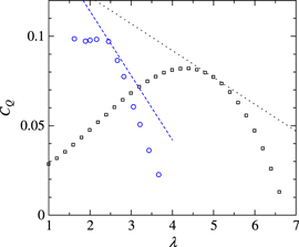
Figure 2. Profiles of  and linear profiles around optimal tip-speed ratio characterized by
  for Toshimitsu et al (2012) and Karasudani et al (2007).Blue and black symbols show profiles for Toshimitsu et al (2012) and Karasudani et al (2007), respectively.
Download figure:
Standard image High-resolution imageThe linear profiles around the optimal tip-speed ratio shown in figure 2 are characterized by the magnitude of the first derivative. The value of the first derivative of  at the optimal tip-speed ratio is calculated by differentiating each form of
  , the values of which are given by differentiating the polynomial approximation for the Toshimitsu et al (2012) CQ profile Karasudani et al (2007) model profile (equation (20)). The magnitudes of the first derivative of CQ at the optimal tip-speed ratio are listed in table 3. As shown in the table, the absolute magnitude of the first derivative obtained by Toshimitsu et al (2012) is larger than that obtained by Karasudani et al (2007). The magnitudes of a2 for the two previous works is also listed in the table. As seen in the table, the magnitudes of a2 cannot be considered to be negligible in comparison to the magnitudes of a1.
Table 3.
Magnitude of  ,
,  ,
,  , CQ, and
  .
.
| Case |

|

|
![$-{{a}_{1}}{{\lambda }_{{\rm opt}}}\;[-]$](https://content.cld.iop.org/journals/1873-7005/47/1/015510/revision1/fdr506646ieqn74.gif)
|
![${{C}_{Q}}\;[-]$](https://content.cld.iop.org/journals/1873-7005/47/1/015510/revision1/fdr506646ieqn75.gif)
|
![$-{{C}_{Q}}/{{a}_{1}}{{\lambda }_{{\rm opt}}}\;[-]$](https://content.cld.iop.org/journals/1873-7005/47/1/015510/revision1/fdr506646ieqn76.gif)
|
|---|---|---|---|---|---|
| Toshimitsu (2012) | −0.036 | −0.15 | 0.091 | 0.092 | 1.02 |
| Karasudani (2007) | −0.015 | −0.026 | 0.077 | 0.077 | 1 |
In the following sections we investigate and discuss the rotational speed response to inflow velocity variation. Through numerical simulation the effect of the differential coefficients on rotational speed response is shown. To calculate the rotational speed response with the torque coefficient profile given by each polynomial approximation numerically, we rewrite the dimensional form of the original equation, equation (1), in the following nondimensional form:

where CQ is the function of the tip-speed ratio based on each form. The numerical solution for the rotational speed  is calculated by integrating equation (22) using the 4th-order Runge–Kutta method. The time increment is set to unity, and the results were not affected by the similar magnitude of the time increment. The maximum time,
  , is set to
  .
.
4. Role of the differential coefficients of the torque coefficient
4.1. Temporal variations of rotational speed response to inflow velocity variation
First we show the results of the temporal variation of rotational speed for the parameters of Toshimitsu et al (2012). The power coefficient profile of Toshimitsu et al (2012) is given for a real wind turbine for the use of wind tunnel testing. In this numerical simulation, there are two formulations of fU which we set. The first formulation consists of a sinusoidal function (Karasudani et al 2010). In this case, fU is formulated as follows,

where  , AU, and T are the velocity variation and constant parameters. Note that the value
  is introduced to equal AU to the rms of fU. The magnitude of AU is set to be
  , and is intended to be the rms of realistic turbulent inflow. We set T = 500, 1000, and 2000, and their magnitudes are similar with those of Toshimitsu et al (2012). The second formulation of
  consists of a random-number sequence whose probability density function is Gaussian. The rms of the normal-random-number sequence is set to be in the same range.
Figure 3 shows temporal variations of fw(t) normalized by  . Note that we normalize fw(t) by
  not by AU because we focus mainly on the amplitude of the sinusoidal-like variation. As shown in figure 3(a), a temporal variation given by the original governing equation has a transient nature which is due to the initial magnitude; with initial magnitude of fw set to be zero. This transient nature is found in temporal variations given by the other governing equations. This nature occurs in the other conditions, as shown in figures 3(b), (c), and (d). In a sufficiently large time, fw(t) varies as a sinusoidal-like variation responding to the sinusoidal variation of the inflow velocity.
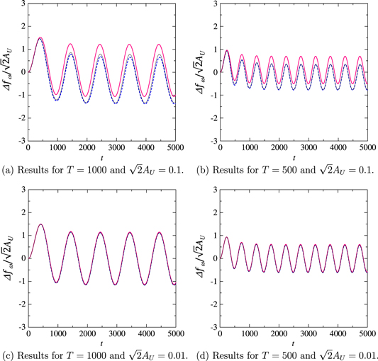
Figure 3. Comparison of results between of the original nonlinear equation and of the modeled equation we derived. The black, dashed-blue, and red solid lines show results of the original nonlinear equation and the equations modeled based on the second-order and the first-order differential coefficients, respectively.
Download figure:
Standard image High-resolution imageThe amplitude of the sinusoidal variation given by the original governing equation is about unity in figure 3(a). The amplitude given by the other governing equation is about unity and agrees with that obtained by the original governing equation. This result implies that amplitude of the sinusoidal variation is not affected by the nonlinear effect, which is first introduced by the second-order differential coefficient. This agreement is found in the other figures 3(b), (c) and (d). Thus, these results suggest that the insensitivity of the amplitude to the nonlinear effect holds for other inflow conditions.
In figure 3(a), there is no phase lag between temporal variations obtained by the original nonlinear equation and the other equations which are modeled by focusing on the differential coefficients. This result is also found in figures 3(b), (c), and (d). This result will be insensitive to flow conditions.
The mean value of the sinusoidal variation given by the linear equation is slightly larger than that given by the original governing equation but this difference can be reduced by adding the leading term based on the second-order differential coefficient. The governing equation based on the second-order differential coefficient is nonlinear and the difference shows that the mean magnitude is affected by the nonlinear effect of the governing equation. This difference is also found in figure 3(b). In contrast to figures 3(a) and (b), in the figures 3(c) and (d) the difference in the mean magnitude is small and can be negligible. From this result, the difference in the mean magnitude depends mainly on the magnitude of AU.
We use a more realistic variation of inflow velocity to compare the rotational speed variation between the governing equations. Figure 4 compares the temporal variation of the rotational speed for the normal-random inflow velocity, where the rms of the normal-random inflow velocity is 0.01. As shown in the figure, temporal variations given by the modeled governing equations are similar to those given by the original governing equation, except for the magnitude of the mean value. The mean magnitude obtained by the linear equation may be found to be slightly larger than that given by the original governing equation. These results agree qualitatively with results for the sinusoidal variation of the inflow velocity.
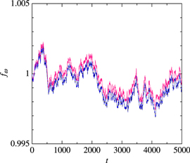
Figure 4. Comparison of instantaneous profile of  . The lines represent the same as that shown in the previous figure.
Download figure:
Standard image High-resolution image4.2. Amplitude, phase lag, and mean value
Nonlinearity is found only in the mean magnitude of the temporal variation of rotational speed as shown in the previous results. To quantify these results, we introduce three parameters:  ,
,  , and
, and  , where the magnitude of these parameters is calculated in a sufficiently large time to avoid transient effects.
  and
and  are the local maximum and local minimum magnitudes, and
  is the phase lag between
  and fU, respectively. Figure 5 illustrates the meaning of these parameters using a sinusoidal variation. The amplitude and mean value of the sinusoidal variation are simply formulated as follows;

Note that the magnitude of the amplitude is equal to the rms of the sinusoidal variation because of the parameter  included in the relation.

Figure 5. Schematic diagram of  ,
,  , and
, and  . The solid and dashed lines show profiles of fU and
  , respectively. Here
  and T = 2000.
Download figure:
Standard image High-resolution imageIn the previous results, the amplitude is found to be insensitive to the nonlinear effect. Figure 6(a) shows rms amplitude profiles depending on the rms of variation AU for three magnitudes of T, T = 500, 1000, and 2000. As shown in the figure, the rms amplitude increases with AU for all magnitudes of T. The profiles given by the linear governing equation agree well with those given by the original governing equation in the whole magnitude of AU, though there may be a slight deviation of the former from the latter. The slight deviation is decreased by adding the leading term based on the second-order differential coefficient for small magnitude of AU. Thus, the slight deviation is due to the nonlinear effect. In the range of large magnitudes of AU, the amplitude for the second-order differential coefficient could not be calculated because the rotational speed diverges. In this regard, the solution to the linear governing equation is more robust than that of the nonlinear governing equation. An additional term which is based on the third-order differential coefficient may be useful to restrain the divergence of the variation.
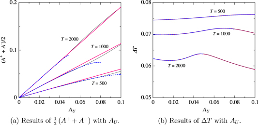
Figure 6. Comparison of the results of the the amplitude and phase lag between the original nonlinear equation and the modeled equation we derived. The meaning of the lines is the same as that shown in the previous figure.
Download figure:
Standard image High-resolution imageThe phase lag between  and fU is less sensitive to the nonlinear effect. As shown in figure 6(b), there is no difference in the phase lag between the original governing equation and the modeled governing equations. This result is found for all magnitudes of T.
In contrast to the results of the amplitude and phase lag, the mean value is affected by the nonlinear effect as noted in the previous results. Figure 7(a) shows the mean value which varies depending on AU. As shown in the figure, the profiles obtained by the linear equation deviate from that obtained by the original governing equation. This deviation is decreased by adding a term of the second-order differential coefficient. This deviation is found for all magnitudes of T.
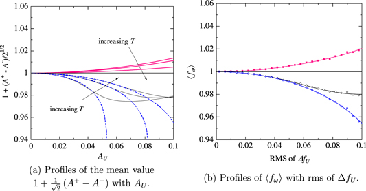
Figure 7. Comparison of the results between the original nonlinear equation and the modeled equation we derived. The meanings of the lines shown in (a) are the same as in the previous figure. The open-circles, blue-open-squares, and red-filled-squares in (b) show the results of the original nonlinear equation and the modeled equations based on the second-order and the first-order differential coefficients, respectively. The solid lines in (b) show the fitting curves.
Download figure:
Standard image High-resolution imageThe nonlinear effect on the mean value is also found in a more real condition. Figure 7(b) compares the mean value of  between the three governing equations in a condition of normal-random inflow velocity. As shown in the figure, the results of the mean value are similar to that of the mean value for the sinusoidal variation.
The above results of the mean value suggest that the nonlinear nature of the governing equation affects the operating point of the tip-speed ratio significantly for large magnitudes of rms of inflow velocity variation. When rotational speed variation is discussed for the range of velocity rms, introducing the additional term will contribute to discussion of rotational speed response in larger magnitudes of the rms. For smaller magnitudes of inflow velocity rms, the governing equation focusing on the second-order differential coefficient as well as the first-order differential coefficient gives accurate results of the mean value. When the mean value as well as amplitude and phase lag are focused on, the linear equation may not be suitable to predict the rotational speed response even if the magnitude of inflow velocity rms is small, because the nonlinear effect is not included in the equation.
All analytical solutions can be given from the linear equation. This is one of the most notable advantages of the use of the linear equation. As shown in these results, the amplitude and phase lag can be predicted with sufficient accuracy even if the nonlinear effect is included. Therefore, the linear equation will be suitable to discuss the nature of rotational speed response when only the two quantities are the focus.
5. Response of  to step input of inflow velocity

5.1. Formulation
The response of  to a step input is a simple issue in addressing the rotational speed response. In this subsection, we address the rotational speed response to a step input of inflow velocity using the equation we derived.
The step input of fU(t) is given as follows:

where  is a constant parameter characterizing the magnitude of the step. The relative rotational speed
  responding to the step input of fU(t) is derived from the equation. A solution of
  is obtained as follows:

where the gain K and time constant τ are derived as follows:

As derived in equations (26) and (28), the rotational speed response is derived as an exact solution of the modified governing equation.
The form of equation (26) is considered to be a form of first-order time lag. Thus, the governing equation derived by focusing on the first-order derivative term of the tip-speed ratio gives the rotational response of the first-order time lag. The solution of the rotational speed response has two parameters: gain K and time constant τ. The two parameters characterize the response of the rotational speed to the step inflow velocity. As shown in the above equation, the form of the time constant τ is rewritten to a form including an energy ratio To. As shown in equation (28), the form of the time constant is simplified using a parameter rim for the formulation.
5.2. Gain
In this study we focus on the magnitude of the gain. As shown in equation (26),  when the presently derived equation is solved, where
  . Figure 8 shows the results of
  as a function of
  for the cases of Toshimitsu et al (2012) and Karasudani et al (2007). Each exact solution agrees with that of the numerical result for the same governing equation. From this agreement, each exact solution can be verified. These exact solutions agree well with the numerical solution of the original nonlinear equation in the region of smaller
  . In the region of large
  , the difference between the exact solution and the numerical solution of the nonlinear equation is larger because the nonlinearity is not negligible, as is found in both cases. The results of the two cases are quite similar to each other.
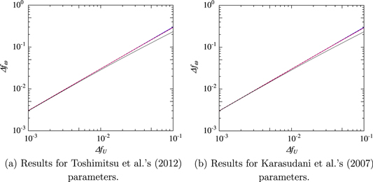
Figure 8. Profiles of  depending on
  , where
  . The black solid lines, red solid lines, black dashed lines, and blue solid lines indicate the numerical results obtained by the nonlinear equation, exact solution of the modified equation, exact solution for small
  , and numerical result of the modified equation, respectively.
Download figure:
Standard image High-resolution imageTo simplify the discussion for the gain K, we additionally derive the first-order approximation of the exact solution for  . The first-order approximation of K for
  is derived as follows:

At the optimal tip-speed ratio, the following relation holds:

Thus,  at the optimal tip-speed ratio. As listed in table 3, the magnitudes of
  of the two previous studies are unity. Using equation (30), equation (29) is rewritten as follows:

As shown in equation (31), the magnitude of K is approximately three.
It should be noted that the magnitude of the first-order approximation of K includes no parameters characterizing the rotational speed response; this term does not include To and  This result suggests that the magnitude of the gain K will not depend on To and
  and is approximately three for this type of common wind turbine.
From equation (26), to obtain the result of the tip-speed ratio from the initial value of the constant tip-speed ratio for  , the following is needed using equation (6):

As derived above, the magnitude of the gain K should be unity to return the tip-speed ratio to the constant tip-speed ratio. As shown in equation (31), the magnitude of the gain K is not equal to unity. This deviation suggests that the tip-speed ratio cannot result in the initial magnitude of the constant tip-speed ratio.
When the magnitude of the constant tip-speed ratio is not optimal,  is not equal to unity. In this case,
  is formulated as
  =
=  . Therefore, the magnitude of the gain Ko at which the tip-speed ratio is not optimal is given as follows:
As shown above, the profile of CP and CQ affects the magnitude of Ko, which is equal to that of K for zero  . This formulation implies that the profile of CP and CQ affects the magnitude of change of the rotational speed owing to the change in the inflow velocity.
The magnitude of  giving
  is not equal to that giving
  . Therefore, the profiles with
  determine whether Ko is smaller than three. In the regions where
  and
and  and
and  and
and  , the magnitude of Ko is smaller than three because the ratio of the differential coefficients in the second terms is positive. In contrast, the magnitude of Ko is smaller than three in the region of
  and
and  because the ratio is negative. This discussion is summarized in table 4.
Table 4.
Magnitude of Ko and sign of  , which are characterized by sign of
  and
and  , where
  =
= ![$3-2\left[ {\rm d}{{C}_{P}}/{\rm d}\lambda {{\mid }_{{{\lambda }_{o}}}}/({{\lambda }_{o}}{\rm d}{{C}_{Q}}/{\rm d}\lambda {{\mid }_{{{\lambda }_{o}}}}) \right]$](https://content.cld.iop.org/journals/1873-7005/47/1/015510/revision1/fdr506646ieqn143.gif) .
.
| Region | Value of Ko | sign of 
|
sign of 
|
sign of 
|
|---|---|---|---|---|
| Region (I) |

|
positive | positive | positive |
| Region (II) |

|
negative | positive | negative |
| Region (III) |

|
positive | negative | negative |
Karasudani et al (2007) discussed the rotational speed response to inflow velocity variation with positive magnitude of the first-order differential coefficient of the torque coefficient. They noted that unrealistic flow field phenomena needed to be assumed for converging rotational speed with positive magnitude of a1. The sign of a1 in region (I) is positive. Thus, this previous discussion suggests that region (I) may not be suitable for wind turbine operation. The first-order differential coefficient of torque coefficient, a1, is positive in this region. For positive magnitude of a1, the magnitude of the time constant is negative, as shown in equation (28). The second term of equation (26) diverges when the time constant is negative. Thus, the present wind turbine will not operate properly in region (I).
In contrast to the rotational speed response in region (I), the sign of a1 in region (III) is negative. Thus, the second term of equation (26) will converge as t increases. Karasudani et al (2007) showed the similar nature of the rotational speed response for a negative value of a1. Therefore, region (III) is appropriate for the operation of small wind turbines.
In realistic situations,  can be zero. Thus, the second terms of equation (33) cannot be calculated for all magnitudes of
  . Thus, we rewrite equation (33) as follows:
The above relation makes it easier to calculate the magnitude of Ko for all magnitudes of  . Figure 9(a) shows Toshimitsu et alʼs (2012) and Karasudani et alʼs (2007) profiles of Ko. As shown in the figure, the magnitude of both profiles is smaller than three in the region where the tip-speed ratio is larger than the optimal tip-speed ratio. In addition, both profiles of Ko for the two previous works decrease as
  increases.

Figure 9. Toshimitsu et alʼs (2012) and Karasudani et alʼs (2007) profiles of Ko and To, which are indicated by the solid line and blue circles in (a) and by the blue dashed line and black solid line in (b), where Ko is calculated by equation (34), and  is the optimal tip-speed ratio.
Download figure:
Standard image High-resolution imageThis decreasing value of Ko with  is qualitatively related to the profile of To. As shown in equation (17), the value of To decreases as
  increases (figure 9(b)), where we rewrite To as
  . As shown in the figure, the profile of Ko at large tip-speed ratio is qualitatively related to the profile of To.
5.3. Time constant
Figure 10 shows the temporal variation of the rotational speed respondse to a step input of the inflow velocity, where  . As shown in this figure, the results of the exact solution, which are verified by numerical results in the figure, agree well with those of the nonlinear original equation. The magnitude of the difference is relatively around 5%. The results of the exact solution for a small magnitude of
  are also shown in the figure. The difference in the magnitude of the exact solutions is sufficiently small and can be negligible.

Figure 10. Temporal variation of  normalized by
  , where
  . The black solid lines, red solid lines, black dashed lines, and blue solid lines show the numerical results obtained by the nonlinear equation, exact solution of the modified equation, exact solution for small
  , and numerical result of the modified equation, respectively.
Download figure:
Standard image High-resolution image
In a linear-time-invariant system, the time constant plays a significant role because the form of the output response to the input is formulated based on an exponential function including the time constant. The time constant remains a useful parameter even if the system in question is not completely linear-time-invariant. The time constant has been considered a parameter characterizing the response to an input.
The difference of the rotational speed response between the two cases is characterized by the difference in the time constant. The magnitudes of the time constant (equation (28)) for Toshimitsu et al (2012) and Karasudani et al (2007) are approximately  and
and  , respectively. The magnitude of the time constant in Toshimitsu et al (2012) is smaller than that in Karasudani et al (2007).
To simplify the form of the time constant (equation (28)), the form is also approximated as follows:

In contrast to the form of the gain K, the time constant depends on three parameters:  , and
, and  . As shown in equation (35), the magnitude of the first derivative of the torque coefficient directly characterizes the magnitude of the time constant.
Karasudani et al (2007) derived a form of the time constant as follows:

We attempt to relate the present form of the time constant (equation (28)) to the previous form. We rewrite this form with a slight modification, which focuses on  rather than on
  , as follows:
where ![${{\tau }_{u}}\;[-]$](https://content.cld.iop.org/journals/1873-7005/47/1/015510/revision1/fdr506646ieqn170.gif) is a nondimensional form of the time constant with the characteristic quantities in Karasudani et al (2007). Using equation (30), equation (37) at the optimal tip-speed ratio can be rewritten as follows:
is a nondimensional form of the time constant with the characteristic quantities in Karasudani et al (2007). Using equation (30), equation (37) at the optimal tip-speed ratio can be rewritten as follows:

This form of the time constant is the same as that of equation (28) with the condition that  . The present time constant is the same as the time constant for small magnitudes of
  in Karasudani et al (2007). In addition, the Karasudani et al (2007) time constant is noted to be a specific case of the present time constant with sufficiently small magnitude of velocity variation
  . As mentioned in this subsection, the previous form of the time constant is a specific case of the present form of the time constant.
The time constant is related to the power of wind turbines. At the optimal tip-speed ratio, the present form of the time constant is rewritten for zero magnitude of  as
as

As shown above, the time constant is directly related to the power coefficient CP. Using a dimensional form of the time constant,  , from the above form of τ, the following is obtained:

where P is the power of a wind turbine, and there exists the relation  . Thus, from the above relation, the form of the time constant is interpreted to imply an integral time relating aerodynamic characteristics to characteristics of the rotating rotor of a wind turbine.
6. Conclusions
In this study, we formulated the rotational speed response to varying inflow velocity for small wind turbines. With this formulation of rotational speed response we derived a differential equation modelled by focusing on the first- and second-order differential coefficients of the torque coefficient profile. Then, we discussed the rotational speed response using the simplified differential equation.
A differential equation is given from the governing equation of the rotational speed response using the parameters of the torque coefficient profile. By using the expansion of the torque coefficient profile for the derivation of the tip-speed ratio, this differential equation, which includes first- and second-order differential coefficients of torque coefficient, was derived. This differential equation is nondimensional, and the nondimensional parameters of this equation are  and constant tip-speed ratio
  , where I,
  , ρ, R, and Uo denote the inertia moment, rotational speed, air density, actuator disk radius, and inflow velocity, respectively. The derived differential equation is found to be a first-order linear equation when the first-order differential coefficient is only included. The second-order differential coefficient produced a part of the nonlinear effect of the governing equation.
First we examined the role of the first- and the second-order differential coefficients. We compared the numerical solutions for the linear equation, the nonlinear equation based on the second-order differential coefficient, and the original nonlinear equation. In this numerical simulation, we simulated the temporal variation of rotational speed response to sinusoidal and normal-random variations of inflow velocity. The amplitude and phase lag of the rotational speed are well predicted by the linear equation as well as the nonlinear equation. The nonlinearity mainly occurs in the mean value of rotational speed.
We derived a solution of the rotational speed for a step input of inflow velocity, and the form of this solution was found to be the same as that of first-order time lag. The magnitude of the derived solution of the linear equation is comparable with that of the original nonlinear governing equation, which is numerically solved for the conditions of two previous studies (Toshimitsu et al 2012, Karasudani et al 2007). The gain and time constant of the first-order time lag were formulated. For small magnitude of step inflow velocity, the magnitude of the gain is independent of To,  , and the first-order differential coefficient of CQ, and is found to be three when the tip-speed ratio is optimal. In contrast to the form of the gain, the time constant is found to be a function of the three variables. Through a discussion of the physical meanings of this derived form of the time constant, the time constant is interpreted as an integral time that relates the aerodynamic characteristics of the rotor to the characteristics of the rotating rotor of a wind turbine.
Acknowledgments
The authors acknowledge Associate Professor T Ushijima (Nagoya Institute of Technology) for his valuable comments on this study. Part of this study is supported by the Japanese Ministry of Education, Culture, Sports, Science and Technology through Grants-in-Aid (No. 25420115).