

Abstract
Past results have suggested that the drag coefficient and the shedding frequencies of regular polygon plates all fall within a very narrow band of values. In this study, we introduce a variety of length scales into the perimeter of a square plate and study the effects this has on the wake characteristics and overall drag. The perimeter of the plate can be made as long as allowed by practical constraints with as many length scales as desired under these constraints without changing the area of the plate. A total of eight fractal-perimeter plates were developed, split into two families of different fractal dimensions all of which had the same frontal area. It is found that by increasing the number of fractal iterations and thus the perimeter, the drag coefficient increases by up to 7%. For the family of fractal plates with the higher dimension, it is also found that when the perimeter increases above a certain threshold the drag coefficient drops back again. Furthermore, the shedding frequency remains the same but the intensity of the shedding decreases with increasing fractal dimension. The size of the wake also decreases with increasing fractal dimension and has some dependence on iteration without changing the area of the plate.
Export citation and abstract BibTeX RIS
Communicated by A Gilbert
1. Introduction
The flow around regular polygon plates has been studied numerous times in the past, the most common of which has been the axisymmetric circular disc; however, several studies have also focused their attention on square plates. This is not to say that other shapes have not been considered, which is why we provide a brief overview of the numerous studies that have been carried out on regular polygon plates which show that the drag and shedding properties of the wake generated by these plates all fall within a very narrow band of values, as shown in figure 1.
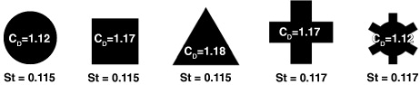
Figure 1. The drag coefficient and Strouhal number for a variety of shapes; the data are taken from Fail et al (1957) except for the cross, which is taken from this study. The Strouhal number is  , where f is the shedding frequency, A is the area of the plate and U∞ is the velocity of the incoming flow.
Download figure:
Standard image High-resolution image1.1. Circular and square discs
Since the first basic flow visualizations of the wake structure behind a circular disc performed by Marshall and Stanton (1931), researchers have focused their attention on understanding this flow in more detail. To the best of our knowledge, Fail et al (1957) obtained some of the earliest measurements of the drag and shedding frequencies of circular discs as well as other plates of similar frontal area. For the circular disc, they found that the drag coefficient was 1.12, while the Strouhal number, St, based on the square root of the frontal area, was found to be 0.115. Carmody (1964) took hot-wire and pressure measurements behind a circular disc showing that 95% of the total transfer of energy from the mean motion to the turbulent motion takes place very close to the plate, usually within the first three plate diameters. Carmody (1964) also offered a CD of 1.14.
So far, the characteristics of the plates had only been considered with a laminar freestream. However, in 1971 Bearman (1971) began looking at the effect that a turbulent freestream has on the drag force on plates. Bearman (1971) studied square and circular discs of different sizes and found the base pressure coefficient, (CP )b, to be −0.363, and that it was the same for both types of plates. With the addition of a turbulent freestream, the base pressure decreased and with it, the drag coefficient increased. The 8 inch square plate, for example, had a CD of 1.152 with a laminar freestream, but this then increased with a turbulent freestream, typically by a few per cent.
The influence of a turbulent freestream on the drag of plates was further studied by Humphries and Vincent (1976a, 1976b), who found that the drag of a circular disc could be increased up to 1.28 as the turbulent intensity and integral length scale in the turbulent freestream are increased. These studies as well as that by Bearman (1971) suggested that the reason for the increase in drag was due to a delay of the shear layer's transition to turbulence, which would keep the base pressure low and hence increase the drag.
Some further progress in understanding the wake structure was made by Berger et al (1990), whose experiments focused on the near wake at relatively low Reynolds numbers and revealed various regimes with various associated shedding frequencies. Further studies by Lee and Bearman (1992), Miau et al (1997), Kiya et al (2001) and Shenoy and Kleinstreuer (2008) have added to the understanding of the wake of a circular disc; however, as stated by Kiya et al (2001): 'the wake of a square plate normal to the flow is not understood yet'.
1.2. Other polygon-shaped discs
Although the study of regular polygon plates has been dominated by circular discs as well as square plates, a few other shapes have also been considered. Fail et al (1957), besides studying these two plates, also studied an equilateral triangle plate and a tabbed plate—all four plates used by Fail et al (1957) are shown, scaled, in figures 4(k)–(n). What was rather surprising was that all these plates had similar drag coefficients between 1.12 and 1.15 and Strouhal numbers between 0.115 and 0.117 when the incoming flow was laminar. A similar CD value of 1.18 was found by Humphries and Vincent (1976b) for the triangular plate with a laminar freestream.
Elliptical and rectangular plates were studied by Kiya and Abe (1999) and again by Kiya et al (2001), where the main finding was that the wake had the same shape as the plate itself; however, the alignment is rotated by 90° with the major axis of the plate aligned with the minor axis of the wake. Two distinct shedding frequencies are also observed, one for each axis; however, the Strouhal number is found to decrease with aspect ratio of the plate, from roughly 0.12 where the aspect ratio is 1, to roughly 0.06 for the major axis and 0.11 for the minor axis of an elliptical plate with an aspect ratio of 3.
1.3. Large-scale or small-scale effects?
From the literature, it is clear that both the drag coefficient and the Strouhal number of circular discs and regular polygon plates appear to fall within a very narrow band of values, with the difference between their CD values being, at most, not more than 5%. Even the tabbed plate, which could have three defined length scales: one associated with the inner diameter, one with the outer diameter, i.e. including the tabs, and the tab itself, has a similar CD and St. This plate is of particular interest, as one would expect the tabs to somehow interact with the shear layer that may change its transition point and with it the drag coefficient, as suggested by the arguments of Bearman (1971) and Humphries and Vincent (1976a, 1976b). This, however, is not the case, as Fail et al (1957) show that the circular plate and the tabbed plate have the same value of CD = 1.12. The question then becomes: if more length scales are introduced, could that cause a change that would create a larger drag coefficient?
If an energy balance is done between the work required to move a plate through a fluid in the direction normal to its plane, and the dissipation of the turbulent kinetic energy that is produced in the fluid (see the appendix), then the following expression can be obtained:

where the wake volume coefficient is defined as CV = Vwake/2A1.5, Vwake being the volume filled by the wake, A is the frontal area of the plate and  is the coefficient of the average rate of dissipation of turbulent kinetic energy in the volume of the wake, as defined by

It is now apparent with (1) that the drag of a blunt object can be controlled either by changing the dissipation in the wake or by keeping constant the dissipation but somehow changing the size of the wake or even a combination of the two. This also poses the question of whether the volume of the wake can be changed without changing the area of the plate. Here we show that it is possible to achieve this, thus manipulating the drag, by introducing a range of length scales on the edge of the plate without changing the area. The purpose of this study is to investigate these phenomena. We use fractal geometries to introduce a variety of length scales to the edge of a square plate. In doing so, we follow recent works by, e.g., Seoud and Vassilicos (2007), Kang et al (2011) and Laizet and Vassilicos (2012), amongst others (see an exhaustive list of references in Gomes-Fernandes et al (2012)). In particular, Kang et al (2011) measured drag forces of Sierpinski carpets and triangles, similar to the shapes used by Abou El-Azm Aly et al (2010) and Nicolleau et al (2011), who investigated the pressure drop across fractal-shaped orifices. Laizet and Vassilicos (2012) showed that the pressure drop across a space-filling (Df = 2) fractal square grid is much lower than that across a regular grid with the same blockage and the same effective mesh size.
2. Experimental setup
Over the course of this study, two wind tunnels were used. The 'Honda' wind tunnel in the Department of Aeronautics at Imperial College London has a working cross-section of 5 ft × 10 ft, a length of 30 ft and a top speed of 40 m s−1. The second tunnel was the 'Donald Campbell' (DC) tunnel, again at Imperial College London, which has a working cross-section of 4 ft × 5 ft (1.22 m × 1.52 m), a length of 11 ft (3.35 m) and a top speed of 40 m s−1. The blockage ratio, i.e. the ratio between the frontal area of the plate to the cross-sectional area of the test section, was found to be 1.41% in the 'Honda' tunnel, while it was 3.53% in the DC tunnel. Background turbulence levels in the Honda and DC tunnel were found to be 0.3 and 0.23%, respectively.
The basic setup in both tunnels included a stand with a protruding arm onto which the plates were mounted. For the Honda measurements, this extrusion was an iml Z-type 500 N load cell which has a total inaccuracy of < ± 0.05% of full-scale range, while in the DC tunnel, the iml sensor was used as well as a more accurate six-axis ATI Nano17 force/torque sensor, which was attached on the end of a 100 mm steel rod—see figure 2(b). This sensor has a range of 35 N in the direction of the drag force and a resolution of 1/160 N, but is also capable of measuring the moments about three axes with a resolution of 1/32 N mm. In the DC tunnel, force/torque measurements were taken for a range of free-stream velocities, U∞, from 5 to 20 m s−1 in 2.5 m s−1 intervals, with data sampled for 60 s, which was satisfactory for converged statistics of the mean and fluctuating values. A single set of measurements at U∞ = 20 m s−1 were taken in the Honda tunnel.

Figure 2. Schematic representation of the experimental setup in (a) the Honda wind tunnel with both side and front views and (b) the side on view in the DC tunnel.
Download figure:
Standard image High-resolution imageHot-wire and pressure measurements were taken downstream of the plates. A rake of Pitot tubes, in a 2 × 10 matrix spanning a distance of 450 mm and a spacing of 50 mm, was placed on the traverse in the DC tunnel. The rake was then traversed vertically in the y-direction to get a two-dimensional (2D) plane of measurements, creating a 10 × 10 matrix of data points, covering a distance of 450 mm in both directions and a spacing of 50 mm between successive points. This spacing gave a ratio of probe diameter to probe spacing of 10, which was deemed to be sufficient for avoiding interference effects. Measurements of the pressure were taken for a series of downstream locations from two to eight characteristic lengths, which is defined as the square root of the frontal area of the plates. The Pitot tubes were connected to a 32 channel Chell pressure transducer, with the static pressure in the tunnel being taken as the reference for all the measurements. The hot-wire probe is made up of a platinum–rhodium alloy wire (90–10%) etched to a diameter of 5 μm, and is connected to a Dantec Dynamics miniCTA with an overheat ratio set to 1.5.
2.1. Definition of fractal edge geometries
The fractal dimension, Df, is defined mathematically by equation (3) (see Mandelbrot (1983)) and measures how rough or smooth an object is. For a line in a 2D plane, a value of 1 would mean a smooth straight line, while any value greater than 1 would mean a rough shape, the maximum value of Df being 2. The parameters defining the fractal edges of our plates are


where r is the ratio between successive lengths, Pn is the perimeter of the plate at iteration n and S is the number of sides on the base shape on which the fractal edges are applied (S = 4 for a base square plate). A simple way to understand the fractal shape of the edge is illustrated in figure 3. The base straight line of length λ is replaced by a number, d, of segments of length l1 such that the area under the line remains the same. This is iteration n = 1. The second iteration n = 2 consists of replacing each individual segment of length l1 by the same pattern of d segments, but smaller, i.e. the segments now have a length l2 = l1/r. And so on for as many iterations as required. A total of eight 'fractal plates' were manufactured, as well as a square and a cross plate. The fractal plates are based on a square plate of 256 mm × 256 mm × 5 mm size, 5 mm being the thickness of the plate, and were designed such that the area remained constant, achieved by a simple 'add on and take away' method as in the example of figure 3.

Figure 3. Illustration of a fractal iteration with corresponding definitions of fractal parameters. (a) Df = 1.5 and (b) Df = 1.3.
Download figure:
Standard image High-resolution imageTwo patterns were used to generate the fractal plates, a square (α = 90°, d = 8 and Df = 1.5) and a triangle pattern (α = 45°, d = 4 and Df = 1.3), with the square pattern shown in figure 3. Consecutive iterations were obtained by applying the same pattern to each new length scale generated, repeated up to four times, giving four plates for each pattern as can be seen in figure 4. It can also be seen from this figure that the fractal plates no longer resemble a square, but more of a cross shape, hence a cross plate was also manufactured. The same figure also has scaled drawings of the plates used by Fail et al (1957).

Figure 4. Scaled drawings of the flat plates used in this experiment, as well as those used by Fail et al (1957). The frontal areas for panels (a)–(j) are identical. Note that the plates were mounted in the tunnel with the orientation shown above, with the vertical and the spanwise axis shown in panel (a). (a) Square, (b) cross, (c) Df1.3(1), (d) Df1.3(2), (e) Df1.3(3), (f) Df1.3(4), (g) Df1.5(1), (h) Df1.5(2), (i) Df1.5(3), (j) Df1.5(4), (k) square used by Fail et al (1957), (l) circle used by Fail et al (1957), (m) triangle used by Fail et al (1957) and (n) tabbed used by Fail et al (1957).
Download figure:
Standard image High-resolution imageAlthough all the plates have the same frontal area, the perimeter (Pn) varied as can be seen in table 1, where the perimeter can be anything up to 16 times longer than the original square plate. It is by applying a fractal pattern that we are able to introduce a larger perimeter and different length scales into the flow without changing the area of the plate.
Table 1. Fractal plate dimensions—Df is the fractal dimension, n is the iteration of the fractal pattern, P is the perimeter given in metres and ln is the length of each segment at the given iteration in mm.
| Name | Df | n | P (m) | ln (mm) |
|---|---|---|---|---|
| Square | 1.0 | 0 | 1.03 | 256.20 |
| Cross | 1.0 | 0 | 1.37 | 114.58 |
| 1.3(1) | 1.3 | 1 | 1.45 | 90.58 |
| 1.3(2) | 1.3 | 2 | 2.05 | 32.03 |
| 1.3(3) | 1.3 | 3 | 2.90 | 11.32 |
| 1.3(4) | 1.3 | 4 | 4.01 | 4.00 |
| 1.5(1) | 1.5 | 1 | 2.05 | 64.05 |
| 1.5(2) | 1.5 | 2 | 4.01 | 16.01 |
| 1.5(3) | 1.5 | 3 | 8.20 | 4.00 |
| 1.5(4) | 1.5 | 4 | 16.40 | 1.00 |
3. Force measurements
3.1. The effect of perimeter and fractal dimension
Figure 5 shows the drag coefficient for the plates, collected in the DC tunnel using both types of sensors, where we can deduce that the change in drag coefficient is not down to the resolution and accuracy of the iml sensor, within acceptable experimental error. Note that the maximum difference between the largest and the smallest drag force measurement is 1.57 N based on a free-stream velocity of 20 m s−1, which is 250 times larger than the resolution of the ATI sensor, which has a resolution of 1/160 N. The largest discrepancy between the two sensors is obtained for the Df = 1.5(4) plate for which we have no definite explanation for the time being; however, despite this discrepancy between the two sensors, conclusions can already be made from this one figure. Firstly, there is a clear effect of iteration within each fractal dimension, which is seen in figure 5 as an increase with increasing perimeter length, and there is an effect of fractal dimension itself. For the Df = 1.3 family of plates, it is only at the last iteration that we see a noticeable increase in CD compared to the square plate of roughly 3.5%, which is similar to the maximum difference between all the plates in figure 1. As the fractal dimension is increased, a more pronounced change in CD is observed, with the Df = 1.5(2) plate showing the biggest increase in CD, roughly 7%. This particular plate can also be compared with the Df = 1.3(4) plate as both sets of plates have the same perimeter, and this shows that by increasing the fractal dimension, one can increase the drag of the plate irrespective of the perimeter length and frontal area, implying that the fractal dimension is a controlling factor in the drag of these plates. The same can be said of the Df = 1.3(2) and the Df = 1.5(1) plates, which also have the same perimeter—see table 1. Special note must also be taken of the cross plate in figure 5, which has the same drag coefficient as the square plate, adding to the evidence that the drag coefficient of non-fractal plates does fall within a narrow band of values.

Figure 5. Change in drag coefficient with perimeter for the square plate ( ), cross plate (+), Df = 1.3 series of plates (
 ) and Df = 1.5 series of plates (
 ). Open shapes refer to measurements taken with the iml sensor and solid shapes refer to measurements taken with the ATI sensor, both in the DC tunnel. There are also two measurements for the cross plate, one for each sensor.
Download figure:
Standard image High-resolution imageOf particular interest in figure 5 is the last iteration of the Df = 1.5 family of plates, where a sharp decline in CD is observed. Hence, two issues must be addressed with respect to the Df = 1.5 family of plates: the initial increase in CD with fractal iteration, and the sudden drop of CD as the iteration increases past a certain value.
3.2. The effect of Reynolds number
Equation (1) shows that the coefficient of drag is independent of Reynolds number,  , as Re → ∞ if in this limit
  and CV are both independent of Reynolds number or if they both depend on Reynolds number in a way that cancels out when one takes the product
  . To check that CD is indeed independent of Re in our measurements, the plates were subjected to a range of velocities in the DC tunnel, ranging between 5 m s−1 ⩽ U∞ ⩽ 20 m s−1. A selection of the results can be seen in figure 6, although it should be noted that all the plates exhibited a Reynolds number independence for Re > 1.5 × 10⁵. The fact that the plates show a consistent trend in the drag coefficient across a range of Reynolds numbers strengthens the support for our conclusions in section 3.1. Even at the lowest Reynolds number the difference between the largest and the smallest force is 16 times larger than the resolution of the ATI sensor, implying that the changes in drag coefficient that we observed are real effects, particularly at higher Reynolds numbers.

Figure 6. Variation of the drag coefficient, CD, with Reynolds number for the square plate ( ), Df = 1.3(4) plate (
 ), Df = 1.5(2) plate (
 ) and the Df = 1.5(4) plate (
 ). Data taken from the DC tunnel using the ATI Nano 17 sensor.
Download figure:
Standard image High-resolution image4. Near wake measurements
While measurements could be taken up to  downstream of the plate in the Honda tunnel, the relatively short length of the test section compared to the size of the plate in the DC tunnel meant that measurements could only be taken for the first eight characteristic lengths. It is in the Honda tunnel that the main bulk of axial measurements are taken, while planar measurements were taken in the DC tunnel.
4.1. Axial pressure and turbulence measurements
Using a Pitot-static probe, the axial pressure, i.e. along the x-direction on the centre line crossing the centre of the plate, was collected for all the plates from  to
to  in the Honda tunnel. Our results, along with those of Carmody (1964) for the circular disc, are shown in figure 7, where the coefficient of pressure is defined as CP = P/(0.5ρU2∞), with P being the dynamic pressure (i.e. total pressure minus static pressure) of the Pitot-static tube in the wake of the plates. Based on these results, it would appear that there is little difference between the square and the cross plate and that even the Df = 1.3(4) has similar pressure coefficient values. The Df = 1.5(4), however, shows a smaller pressure drop close to the plate and a very slow rate of pressure recovery; even at a distance of
  the wake has not recovered to the same levels as the other plates. Although only the fourth iteration of both fractal dimension families are shown, it should be noted that there is a decreasing pressure drop behind the plate for increasing fractal iteration and that further downstream there is a faster rate of pressure recovery as fractal iteration is increased. These results also suggest, judging from the position where CP = 0, that the length of the re-circulating region is roughly similar for all plates; however, no conclusions can be made about the overall volume of the bubble itself.
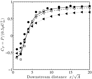
Figure 7. Axial pressure coefficient for the square ( ), cross plate (+), Df = 1.3(4) (
 ) and Df = 1.5(4) plate (
 ) in the Honda tunnel. The figure also shows the data collected by Carmody (1964) for the circular disc (
 ) as well as data for the square plate and the Df = 1.5(4) plate in the DC tunnel (
 ). Lines are added to data points to show the difference between data sets.
Download figure:
Standard image High-resolution imageThe axial evolution of the turbulence intensity, Ti = u'/U∞ where u' is the fluctuating velocity, is shown in figure 8 for the square, cross and the last iteration of both fractal plates where, as before, there is no noticeable difference between the Ti values for the cross and square plates. Here we observe that at the closest position the fractal plates have lower levels of turbulence intensity compared to the square and cross plates; however after  , there is a noticeable change where the fractal plates actually have higher levels of turbulence intensity, and at a distance of
  , the Df = 1.5(4) has the highest level of Ti of all the plates.

Figure 8. Axial turbulence intensity measurements for the square ( ), cross plate (+), Df = 1.3(4) (
 ) and Df = 1.5(4) plate (
 ); data collected in the Honda tunnel.
Download figure:
Standard image High-resolution imageAs in figure 7, figure 8 shows the fourth iteration of both fractal dimension families, which had the lowest turbulence intensity close to the plate and the highest further downstream compared to the other fractal iterations, i.e. the rate of decay decreased as the fractal dimension and iteration increased.
4.2. Planar measurements in the near wake
It is clear that although one could use the axial measurements for direct comparison from one plate to another, the same cannot be said of a single traverse through the wake, as is often the practice with axisymmetric plates. Although the square and cross plates both have reflection and rotation symmetry, they are not axisymmetric and so one must take planar measurements to fully understand the development of the wake. This point is even more critical for the fractal plates which only have rotation symmetry (by 90°). Planar measurements of the pressure coefficient are taken in the DC tunnel.
In equation (1), the wake volume coefficient as well as the dissipation coefficient are defined over all fluid space which is assumed to be infinite; however, in practice, it is not possible to measure these values over an infinite domain of the wake. The volume coefficient in equation (1) can, however, be decomposed into the sum of 2D normal slices through the wake over several downstream locations; that is to say,  , where CA is now defined as

where Awake is the planar, cross-section area of the wake and is the only variable that is a function of x. This area can be approached experimentally in a number of ways; however, for this study, we shall define a length based on a certain fraction of the velocity deficit, Ud in the wake, where the velocity deficit is defined as Ud = U∞ − 〈U(x,y,z)〉 and the corresponding length is the point where the deficit velocity is some fraction, ζ, of the centre-line velocity deficit; that is to say, Ud(x,±yζ,±zζ) = ζUd(x,0,0) (U is the streamwise velocity component of the fluid velocity and the brackets 〈··· 〉 signify an average over time). As we are collecting pressure from the rake measurements, this can also be expressed as

The value of the width was found by fitting a sixth order polynomial to the data and finding the point where the velocity deficit was a certain fraction, ζ, of the centre-line deficit velocity. Note that yζ and zζ are the vertical and spanwise distances from the centre line (see figure 2 for definition), where the pressure coefficient is a certain fraction ζ of the centre-line pressure coefficient. Finally, to obtain an estimate of the wake area, the area in plots such as those in figure 9 was integrated from the origin to newly created data points identified as the white circles in that figure.

Figure 9. Contour plots of CP at a distance of  downstream of the plates, including small circles which are the calculated wake boundary based on ζ = 0.5. (a) Square, (b) Df = 1.3(4) and (c) Df = 1.5(4).
Download figure:
Standard image High-resolution imageAs already mentioned in section 2, the spacing between the Pitot probes on the rake was set to 50 mm; however, to determine whether this spacing was adequate to obtain the area of the wake a preliminary test was done. At a distance of  the rake was traversed by 10 mm in the z-direction (see figure 2 for definition of the coordinates) thus obtaining 40 data points which were 10 mm apart. The width of the wake was found in the same way as described above for both sets of data, i.e. one with 10 data points and another with 40 data points, where it was found that both sets of data gave similar results. It is believed, however, that the accuracy of this method would be lower closer to the plate where the wake is much smaller and hence there are fewer data points available for the polynomial fit. Similarly, this method does not work when there are negative CP values, which is why we show data from
  onwards.
In figure 9, we show the planar pressure coefficient measurements taken in one quarter of the wake for a selection of plates, where the corresponding coordinates of the detected wake edge can also be seen. These boundaries are based on a ζ value of 0.5, i.e. the point where the pressure reaches 50% of the centre-line pressure. From a quick inspection, it appears that the wake of the Df = 1.5(4) is the smallest of all the plates—see figure 9(c), and that, just as was noted in figure 7, it has a very low pressure coefficient in the middle of the wake. We have, for a simple comparison, also plotted in figure 7 the centre-line evolution of the pressure coefficient of the square plate taken in the DC tunnel where good agreement between the two tunnels is observed.
As mentioned earlier a number of values for ζ were looked at, and it was observed that the trend of CA from one plate to another was always consistent irrespective of the value of ζ, as can be seen in figure 10. This does suggest that most of the information in terms of getting a good value for CA can actually be obtained from looking at the point where the pressure reaches 50% of the centre-line pressure. From these results, the impression seems to be that no matter what value of ζ is chosen, the area of wake for the square plate will be the largest, followed by the Df = 1.3 family of plates, although only the last iteration is shown here for clarity. The smallest wake can be seen for the Df = 1.5 family of plates, but it must be pointed out that these results are for one downstream location at  .
.

Figure 10. Coefficient of area, CA, as determined from various values of ζ taken at a distance  for (
for ( ) square, (
 ) Df = 1.3(4), (
 ) Df = 1.5(1), (
 ) Df = 1.5(2) and (
 ) Df = 1.5(4).
Download figure:
Standard image High-resolution imageIf we now look at figure 11, where the growth of the wake is shown, we see a clear pattern emerging between the fractal dimensions at  , with all of the Df = 1.3 family of plates having a smaller coefficient of area for all positions compared to the square plate, but a larger CA compared to the Df = 1.5 fractal plates. This fact is particularly interesting, because if we use the drag coefficients from the DC tunnel, where the planar measurements are taken, then we note that the square, the first three iterations of the Df = 1.3 plates and the last iteration of the Df = 1.5 plates all have similar drag coefficients, but the pressure in the wake and the size of the wake are very different in each case. This means that there must be, as predicted in section 1.3, another effect causing the drag to stay the same even though the areas are different.
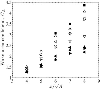
Figure 11. Downstream evolution of the coefficient of area, based on ζ = 0.5 for all the plates, where ( ) square, (
 ) Df = 1.3(1), (
 ) Df = 1.3(2), (
 ) Df = 1.3(3), (
 ) Df = 1.3(4), (
 ) Df = 1.5(1), (
 ) Df = 1.5(2) and (
 ) Df = 1.5(4).
Download figure:
Standard image High-resolution imageFigure 11 gives an indication that the area coefficient changes with iteration, particularly for the Df = 1.3 fractal plates where CA drops for consecutive iterations before increasing again for the last iteration, particularly at the largest value of  .
.
5. Flow shedding
The final aspect of the wake that we study is the flow shedding. From the literature, there appears to be no discernible difference in the Strouhal number ( , where f is the shedding frequency) for the various plates that have been studied, suggesting that the Strouhal number may be independent of the shape of the plate (with the only exception of the circular disc from Berger et al (1990)) generating the wake. By adding so many discontinuities and length scales to the perimeter of the plate, it would be interesting to see whether the shedding changes in any way.
With the single hot-wire probe located at a distance  , measurements were taken at eight polar locations from 0° ⩽ θ ⩽ 315°, with a radius of 200 mm from the axial line (see figure 2) as this position was found to have, on the whole, a stronger signal from the hot-wire for all the plates. It should also be noted that the turbulence intensity in this region was less than 15%. The radial results for the square plate and the Df = 1.5(4) fractal plate, taken at
  , are shown in figure 12, where it can be seen that the power spectral density of the velocity fluctuations for the square plate are consistently higher than the Df = 1.5(4) plate, even though they all shed at the same Strouhal number. It was found that the Strouhal number ranges between 0.11 and 0.12 for all plates, which is in good agreement with previous studies.
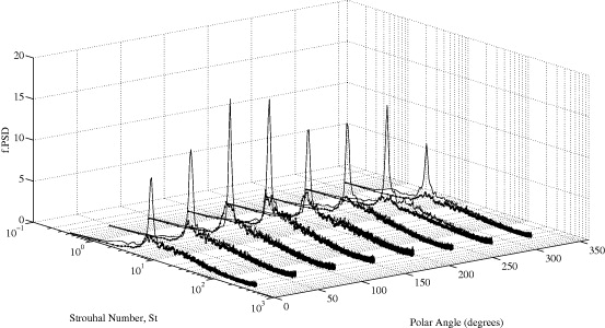
Figure 12. Power spectral density multiplied by f as a function of St at various polar angles for the square plate [ ] and the Df = 1.5(4) fractal plate [
 ], taken at a distance of
  .
.
Download figure:
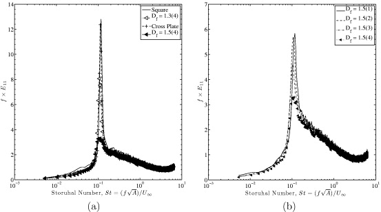
Standard image High-resolution imageThe results therefore suggest that the impact of the fractal geometries on the perimeter of the plates is to diminish the intensity of shedding from the plates, but not the rate at which the flow is shed off the plate. There is even an effect between consecutive iterations and fractal dimension, with the intensity of the shedding diminishing with increasing iteration and fractal dimension, as can be seen in figure 13, where the Df = 1.5(4) has the lowest amount of energy from all the plates by a factor of 4 compared to the square plate. Note that this is based on data for a single downstream and radial location. Fractal edges can therefore presumably be used on plates to very significantly reduce vibration. This aspect will be the object of a future study.
Figure 13. The mean pre-multiplied power spectral density for (a) a selection of plates and (b) for the Df = 1.5 fractal plates at a distance of  . Data collected in the Honda tunnel.
Download figure:
Standard image High-resolution image
6. Conclusion
A non-negligible change in the drag coefficient of up to 7% is observed for flat plates with fractal edges placed normal to an incoming laminar flow. It is therefore possible to change the drag coefficient which was deemed to be insensitive to the shape of the plate's rim from previous studies. This significant change in drag coefficient is insensitive to Reynolds number, but does strongly depend on the fractal dimension, Df, and fractal iteration n.
The energy balance between the work required to move a plate through a fluid and the rate of kinetic energy dissipation in the wake leads to the expression  where CV is a dimensionless volume of the wake and
  is a dimensionless aggregate rate of turbulent dissipation. This equation suggests that the drag of a blunt object can be controlled either by changing the dissipation in the wake or by keeping constant the dissipation but somehow changing the shape of the wake or even a combination of the two. Fractal geometries were used here to create plates for which the volume of the wake can be modified without modifying the area of the plate. The wake becomes smaller as the fractal dimension and fractal iteration are increased.
We also found that increasing the fractal dimension and iteration causes a reduction in the intensity of the shedding, although the frequency at which the flow is shedding does not change.
This paper is, in a sense, introductory and much effort needs to be focused, in future work, on the dissipation properties of these wakes as well as their later sections, such as the intermediate and the far wake, where it is known that the axisymmetric wake becomes self-similar.
Acknowledgments
The authors acknowledge Tianyi Han and Victoria White for obtaining additional force measurements in the Donald Campbell tunnel as part of their Master's projects.
Appendix
A.1. The derivation of equation (1)
Consider a plate moving with constant speed U∞ in a viscous fluid that is stationary at infinity. The work performed in moving the plate against the drag,  , balances the dissipation rate of the kinetic energy of the fluid,
  , where the volume integral is over all fluid space (assumed infinite), the brackets 〈··· 〉 represent a time average and
  (x) is the time-averaged kinetic energy dissipation rate per unit mass, i.e.
  . In this balance, we have neglected a surface integral term representing the energy dissipation rate by surface friction, as skin friction drag is negligible for blunt objects such as plates normal to the flow.
The vast majority of the kinetic energy dissipation resides inside the turbulent wake and the volume, Vwake, of this wake can therefore be used to define an average dissipation by  , where the integral is over the volume of the wake. We define the dissipation rate coefficient
  as
as  , where ℓ is a characteristic length of the object that is creating the wake, defined as
  for our study. The balance between the work performed in moving the plate, which is DU∞, and the dissipation rate
  leads to

where the wake volume coefficient is defined as CV = Vwake/2A1.5 with A being the frontal area of the plate and the characteristic length ℓ being defined as  . A similar relationship can be found for a planar wake, where equation (1) becomes
  , with CA = Awake/A.