


ABSTRACT
Active volcanism observed on Io is thought to be driven by the temporally periodic, spatially differential projection of Jupiter's gravitational field over the moon. Previous theoretical estimates of the tidal heat have all treated Io as essentially a solid, with fluids addressed only through adjustment of rheological parameters rather than through appropriate extension of the dynamics. These previous estimates of the tidal response and associated heat generation on Io are therefore incomplete and possibly erroneous because dynamical aspects of the fluid behavior are not permitted in the modeling approach. Here we address this by modeling the partial-melt asthenosphere as a global layer of fluid governed by the Laplace Tidal Equations. Solutions for the tidal response are then compared with solutions obtained following the traditional solid-material approach. It is found that the tidal heat in the solid can match that of the average observed heat flux (nominally 2.25 W m−2), though only over a very restricted range of plausible parameters, and that the distribution of the solid tidal heat flux cannot readily explain a longitudinal shift in the observed (inferred) low-latitude heat fluxes. The tidal heat in the fluid reaches that observed over a wider range of plausible parameters, and can also readily provide the longitudinal offset. Finally, expected feedbacks and coupling between the solid/fluid tides are discussed. Most broadly, the results suggest that both solid and fluid tidal-response estimates must be considered in exoplanet studies, particularly where orbital migration under tidal dissipation is addressed.
Export citation and abstract BibTeX RIS
1. INTRODUCTION
Earth and Jupiter's moon Io are the only planetary bodies in the Solar System observed to have active silicate volcanism. However, the internal heat sources driving volcanism in these two cases are very different. The Earth contains sufficient radiogenic material to drive these processes, but the primary internal source of heat on Io is thought to be strong tidal action by Jupiter's gravitational field. Following a theoretical study (Peale et al. 1979) that predicted the active volcanism observed by the two Voyager spacecraft, it has generally been assumed that the heating associated with the tidal action is exclusively due to dissipation treated essentially as a solid. Recent reanalysis of Galileo magnetometer data shows that Io has an induced magnetic field, which combined with other constraints implies the presence of a global "magma ocean" (Khurana et al. 2011). Specifically, the cited study concludes that there exists an asthenosphere of thickness 50 km or more and composed of at least 20% interconnected melt. While a layer of complete melt is not precluded, it is more likely that the type of magma ocean on Io is a partial melt layer with interconnected liquid that can flow through a more slowly deformable matrix of solid. The presence of a magma ocean within Io raises the possibility that tidally induced fluid flow could generate substantial dissipative heat. It is known both experimentally and through analyses of the governing equations that solids and fluids respond quite differently to tidal forces. There are typically strong differences in the types of stress supported in each media, and the intrinsic timescales for adjustment may also be quite different. The large differences in timescales can lead, for example, to the retention of inertial terms (including rotational "forces") in the case of fluids, while such components are negligible in the case of solids. However, the tidal responses of the two media should not be entirely distinct as there are similar processes and constraints applicable to both.
The motivation for this study comes from observation that if a global magma ocean is present within Io, previous estimates of tidal dissipation in a solid Io provide an incomplete or perhaps even erroneous description. The goal of this study is therefore to provide a description of the expected fluid tidal dissipation and compare it with that estimated for the solid in an attempt to determine the relative contribution of each. There are, however, uncertainties in the choice of appropriate parameters and model formulations in each case. Because of this, a proximate goal is to describe the behavior and parameter dependencies in each case such that distinguishing elements of the two process may be separated and ultimately used to estimate the respective roles of the solid and fluid phases in Io's tidal dissipation.
The hypothesis that tidal dissipation within fluid layers may contribute significantly to the overall energy loss budget for a planetary object has wide reaching implications not only for the early tidal and spin evolution of moon systems within our own solar system, but also for planets and moons in the growing catalog of extrasolar planetary systems. In particular, by providing a major second possible source of dissipation, fluid tides provide a possible mechanism to significantly increase orbital damping rates beyond those predicted by solid-tidal models alone. Early solar systems often experience high rates of scattering (e.g., Mandell et al. 2007; Nagasawa et al. 2008; Raymond et al. 2009), whereby larger perturbers may increase the eccentricities of terrestrial-class objects (e.g., Weidenschilling & Marzari 1996; Chatterjee et al. 2008; Matsumura et al. 2008; Shen & Turner 2008; Matsumura et al. 2010). Increasing tidal dissipation may be highly beneficial for Earth-class objects in such systems (Henning & Hurford 2014), by allowing orbital circularization to proceed more rapidly, and thereby reducing the timespan over which such worlds remain vulnerable to orbit crossings and resonances that can lead to ejection from the stellar system or absorption into the host star (Matsumura et al. 2013). Adding fluid tidal heating to models may therefore help to improve survival rates of terrestrial class objects in chaotic early solar systems. Note that young silicate objects recently following accretion, as well as objects with high eccentricities, are those for which silicate magma fluid layers are more likely (e.g., Elkins-Tanton et al. 2003). While not treated in detail here, dissipation increases due to non-silicate liquid layers, such as surface or subsurface water oceans, may have similar orbital consequences.
Returning to Io and the potentially observable differences between fluid and solid tidal heat generation, an example of distinct behavior, which will be discussed next, involves the global distribution of the tidal dissipative heat flux. For plausible parameter scenarios, the distribution of the dissipative heat generated differs between the two types of tidal process. These calculated distributions of dissipative heat may be related to observations of the surface heat fluxes. If volcanic centers are directly correlated with surface heat flux, then the spatial distribution of volcanoes on Io provides criteria that may be used to isolate the type of tidal process most active on this moon. Estimates of Io's global mean heat flow generally range from 1.5 to 4.0 W m−2 (Moore et al. 2007), with recent astrometric observations supporting a value of 2.24 ± 0.45 W m−2 (Lainey et al. 2009). However, most of this heat is carried to the surface by ascending silicate magma rather than by conduction through the lithosphere (McEwen et al. 2004). The heat-pipe mechanism proposed for transporting Io's internal thermal energy to the surface (O'Reilly & Davies 1981) involves bringing magma upward through hotspots or "heat pipes" that are embedded within a relatively cold lithosphere. Focusing of upwelling magma through the lithosphere is important because it discretizes surface heat flux patterns that are expected from tidal dissipation models. Kirchoff et al. (2011) examined the global distribution of volcanoes on Io using spherical harmonic analyses and identified statistically significant clustering at spherical-harmonic degrees 2 and 6. Applying an optimized distance-based cluster analysis to the locations of hotspots and paterae identified in the first 1:15,000,000 global map of Io (Williams et al. 2011a, 2011b), Hamilton et al. (2013) determined that there is a 30°–60° eastward offset in concentrations of volcanism on Io relative to the surface heat flux maxima predicted by conventional tidal dissipation models, which consider that heating is primarily due to solid-body dissipation in the asthenosphere. It should be pointed out that it is unclear how reliably this observed offset reflects an offset in subsurface heat fluxes. Indeed, a reliable mapping of the subsurface heat sources that produce the surface distribution is not straightforward and the analyses and scope of potential candidates are not presented here. Further studies focused on such mapping would be valuable. Here we provisionally assume that an offset in the subsurface heat sources is suggested though not confirmed by observations. That we demonstrate a tidal heating process that in fact allows such offset will evidently be relevant in developing such mapping.
In all previous studies, tidal dissipation within Io has been assumed to be due to deformation of solid or partially molten material (Peale et al. 1979; Ross & Schubert 1985, 1986; Segatz et al. 1988; Ross et al. 1990; Tackley 2001; Tackley et al. 2001). The tidal force used has only included the equatorially symmetric degree-2 spherical-harmonic terms representing the leading terms in a Taylor expansion of the gravitational potential associated with Io's eccentric orbit. In a related context, Tyler (2008) has emphasized that even in the case where it is a relatively weak component, the tidal force associated with axial tilt (obliquity) must also be examined when calculating fluid tides because inertial effects in the fluid lead to a tidal response that is not necessarily commensurate with the tidal force amplitude. In this case a relatively weak obliquity tidal force can be responsible for even the dominant part of the tidal flow response. However, in the application here, where eccentricity is 0.0041, obliquity is likely to be a small fraction of a degree, and the fluid tidal response is expected to be heavily damped (forbidding a sharply resonant response), it is expected that the conditions for this disproportionate response due to resonances is not met and only the eccentricity tidal forces are considered in detail. Peale et al. (1979) showed that at least a significant fraction of tidal heat may be expected from theoretical estimates assuming reasonable values of the unknown dissipation parameter Q and the Love number  . Subsequent refinements of this work (Segatz et al. 1988; Ross et al. 1990; Tackley 2001; Tackley et al. 2001; Turcotte & Schubert 2002; Moore et al. 2007) have sought to better match dissipation estimates from radiometry to interior models. In end-member tidal dissipation models, the bulk of Io's heating occurs either within the deep-mantle or within the asthenosphere (Ross & Schubert 1985, 1986; Segatz et al. 1988; Tackley 2001; Hamilton et al. 2013), while in mixed models heating is partitioned between these end-members (Ross et al. 1990; Tackley et al. 2001; Hamilton et al. 2013). In deep-mantle heating models, the flux of heat through the surface is maximum near the poles and minimum at the equator, with absolute minima occurring at the subjovian and antijovian points. In asthenospheric models, heat flux is minimum at the poles and maximum in the equatorial area, with primary maxima occurring north and south of the subjovian and antijovian points (at approximately ±30° latitude), and secondary maxima occurring at the centers of the leading and trailing hemispheres. Spatial variations in surface heat flux are lower in mixed models, with maxima migrating toward the poles as deep-mantle heating is added to asthenospheric heating.
In Section 2, we describe the methods used to calculate the tidal dissipation under the respective models of a thin fluid magma ocean, and a solid that may include melt. Of course, within each of the two model frameworks there are really a range of solutions because the parameters required in the calculations are poorly constrained. Each one of these solutions comprises a complete set of solution variables, but for the purposes here the solution variable of interest is the rate of work performed by the tidal forces on the medium. The rate of work performed describes the level of tidal excitation, and it is also assumed that global/temporal averages of this work rate correspond to rates of dissipative heat generation. The analyses then involve describing the tidal heat generation (the solution variable) as a function of the unknown parameters. When first only the global integral (or surface average) is needed, the solution variable is then represented as a scalar function represented in a parameter space involving the unknown parameters as coordinates. An attempt is made to combine these parameters into degenerate non-dimensional combinations to provide the most compact space of solution scenarios. When analyses shift toward examination of the spatial distribution of the heating rate, then the approach is to select end-member examples from the behavior seen in the space of solutions. In Section 3, we summarize results describing the behaviors of the two families of tidal-response solutions calculated using the methods in Section 2. In Section 4, we isolate and describe subsets of the solutions from Section 3 which satisfy primary observational constraints (e.g., total heat flux), and then discuss differences in behavior (e.g., the distribution of the heat flux) that may be used as further observational criteria for distinguishing between the tidal processes active on Io. Finally, conclusions are summarized in Section 5.
2. METHODS
2.1. Calculation of the Tidal Response of the Solid
We compute tidal dissipation in a layered self-gravitating solid body using the propagator matrix method (Love 1927; Alterman et al. 1959; Takeuchi et al. 1962; Peltier 1974) presented in comprehensive detail in Sabadini & Vermeersen (2004). This technique assumes a model domain composed of spherically symmetric shells, each with prescribed density, shear modulus, and viscosity, and applies an external gravitational potential (here a spherical-harmonic degree-2 tidal disturbance; Henning & Hurford 2014). Boundary conditions are solved at each interface to yield solutions for the radial and tangential displacements and stresses. This method traditionally handles boundary conditions for solid-solid interfaces. Our analysis was extended using the TideLab suite of code (Moore & Schubert 2000), that uses techniques documented in detail in Wolf (1994), as well as by alternate methods described in Jara-Orué & Vermeersen (2011; using a Fourier and Laplace approach respectively). These methods handle layer interfaces with static liquid layers, which propagate neither displacement nor stress. The TideLab code utilized generated surface Love numbers, but not spatial patterns, and therefore was used to validate the premise (Henning & Hurford 2014) that weak solid layers are a reasonable approximation for the decoupling of true liquid layers (and may in fact better represent the model of a magma slush). While this approach permits some of the important effects of a fluid, such as the uncoupling of layers, the fluid represented may be considered to be more of a lubricant than a dynamical fluid capable of inertial resonant excitation. The fluid treated here has then less dynamical freedom than that in Section 2.2 and may be regarded as a strengthless medium having gravitational mass but no inertial mass. This apparent breach of the Equivalence Principle is permitted for sufficiently low frequencies where a quasi-static balance of forces prevails and inertial accelerations are small. The solution for the system of concentric viscoelastic shells is found by computing the purely elastic solution to the resulting system of equations, then invoking the viscoelastic-elastic correspondence principle (Biot 1954; Peltier 1974). For continuity with previous studies (e.g., Henning et al. 2009), a Maxwell rheology is used. For a cyclically driven system, the displacement field is converted into a strain-rate field. The propagator solution coefficients for the unit stress and strain-rate fields are then represented by full 9 by 9 element tensors in spherical coordinates for the degree-2 external tidal potential. These are then combined to determine the work per unit volume. In the analogous viscoelastic solution, using the Fourier tidal approach, solutions are complex values where the imaginary component of the computed work represents the energy lost per cycle and thereby the tidal dissipation rate. The time-averaged tidal dissipation from this method is provided as a function of latitude and longitude, just as for the fluid in Section 2.2, but the dissipation is also distributed radially over the concentric shells. We sum the dissipation over the shells to represent a useful first approximation of the equilibrium surface flux of heat prior to re-distribution into heat pipes, perhaps at the base of Io's lithosphere. Beuthe (2013) presents a highly efficient method for calculation of spatial patterns of tidal heating for multilayered planetary objects, with the advantage of being able to explain the range of observed patterns as arising from weighed sums of three fundamental spatial patterns. Results presented in Section 3.1 specifically for Io, are in agreement with this previous work, but are shown for the purpose of linking specific input parameters (mainly layer thickness and viscosities) to the specific patterns and heat magnitudes they achieve.
2.2. Calculation of the Tidal Response of a Fluid Magma Ocean
The "Laplace Tidal Equations" were established very early within the practice of modern science to describe the dynamics of fluid tides on Earth, and there has been a long history of development (Lindzen & Chapman 1969; Longuet-Higgins 1968; Hough 1898; Cartwright 1999). These equations describe the behavior of a fluid flowing in a relatively thin shell such that approximations provide useful simplifications that allow tractable solutions. These equations are widely used to study tides in the terrestrial ocean and atmosphere, but the applications to planetary problems are fewer and more recent. Instead, many planetary applications have followed approaches based on that for solid tides described above, even when fluids are present. An immediate indication that the latter approach may be incomplete when treating a fluid can be seen by inspecting the dynamical terms included or absent in the two sets of governing equations. Unlike the equations used to describe the solid tides, the Laplace Tidal equations include inertia and thereby a resonant response is permitted. More subtle is the effect of rotation which is explicitly represented in the Laplace Equations and has the interesting effect of scattering energy among wave numbers, such that the spectral distribution (as well as the amplitude) of the response need not be commensurate with that of the forcing. In this case, there is not a single Love number relating a tidal forcing component with the fluid's response. This was shown mathematically by Hough (1898) in demonstrating that representation of the Eigenfunctions of the Laplace Tidal Equations (now called "Hough functions") involve a non-trivial series of spherical harmonics. Lindzen (Lindzen & Chapman 1969) elaborated on this in showing that terms associated with negative eigenvalues must be included in the series for a complete representation of general solutions.
The general expectation is therefore that solids and fluids will respond differently to tidal forces, and previous consideration of tides on Io are therefore incomplete if the presence of a magma ocean is accepted. In the specific application we shall present, there may be more similarity between fluid and solid tidal responses than would be generally expected. The reason for this is that we expect that the tidal response of the fluid magma is heavily damped and the response falls in the regime of "creeping flow" where inertial and rotational effects are subdued by friction. Even in this case, the fluid and solid response to tides behave differently because of the different types of stress that each support, and because the fluid is confined to a thin shell. Because of the difference in material properties, a larger surface displacement is typical of the fluid response, and because of the thin shell, relatively strong flow speeds are required by continuity to fill these displaced surfaces. Details of the formulation and method we use for solving the Laplace Tidal Equations has been previously described (Tyler 2011). Briefly, the method is a semi-analytical approach involving a spherical-harmonic expansion and numerical inversion of the coefficient matrix. The only numerical parameter to be chosen is the degree for the truncation, and this is easily taken to be a large value (500) upon which the solution elements discussed have become independent. While the results for this study were obtained through full solutions of the Laplace Tidal Equations, the reader may verify that these solutions show correct overlap with solutions that can be obtained from a much simpler formulation which we include in the
While the equations used here in treating Io's magma ocean are dynamically more complete than in any previous treatment of this or a similar application, there are limitations of the formulation and/or expected additional dynamical components expected. An immediate assumption is that material properties in Io, including the parameters describing the magma layer, are radially symmetric. This is obviously a simplifying assumption. The Laplace Tidal Equations do not require that the parameters be symmetric but the method of solving these equations in this study does. With this symmetry, the thin-shell (also called "long-wave") assumption in these equations is quickly justified for any fluid thickness much smaller than Io's radius (the horizontal length scale of the tidal forcing and tidal response). However, without at least a predominance in this presumed symmetry, the thin-shell assumption may break down and the basis for the equations used must be re-examined. Another factor is the omission of the dynamical effect of the overlying lithosphere on the magma ocean tidal response. This consideration is directly analogous to that of the effect of an overlying ice shell on a water-ocean tidal response and has been discussed in CITE. The argument for postponing any detailed explicit modeling of the coupled dynamical response of the shell and fluid is the same in this study. First, if the upper shell is relatively thin relative to the fluid thickness (e.g., as expected for Europa), then scaling shows that the upper shell is primarily simply floating and does not much alter the fluid's tidal response. The upper shell can of course be thermodynamically important in controlling the rate of heat loss, but it is not, to first-order consideration, important mechanically in the fluid's tidal response. Second, even if the upper shell is relatively thick (e.g., as expected for Ganymede, Callisto), the first-order effect of the shell is simply to damp the tidal response, and this effect is therefore included (parameterized) in such studies as in CITE or here where the damping timescale is treated as a free parameter.
3. RESULTS
3.1. Tidal Dissipation in the Solid
For the solid tidal dissipation solutions, the general form of the surface expression is controlled by the layer structure, and primarily by the viscosities and thicknesses assigned. Pervious work (e.g., Segatz et al. 1988) has suggested solid dissipation in Io is expected primarily in a higher melt-fraction asthenosphere/upper mantle, with moderate heating occurring in Io's mid- and lower-mantle. Tidal dissipation from the Ionian crust is largely negligible due to the expected high viscosity of such a colder lithosphere, as well as due to the very small global volume of crustal material. Io's Fe or FeS core is expected to be fully molten, with a very low viscosity, thus contributing negligibly to dissipation from non-inertial deformation.
In Figures 1 and 2, we present six cases of solid tidal dissipation for comparison with the fluid tidal solution. Figure 3 shows the distribution of tidal heating as a function of depth throughout Io for the same six example cases. In each case, the material parameters have been selected such that the total global dissipation rate matches the nominal 2.25 W m−2 level of observations. Previous investigations have noted that it is difficult for solid tidal dissipation to account for all of Io's observed heat flux. By setting the totals in Figure 1 to match observations we have taken the opposite approach and asked what material parameters are necessary for solid tides to reach this level. The difficulty of previous work in matching observations with solid dissipation alone, arises due to the necessity to stretch the expected range of viscosities and layer thicknesses beyond values traditionally tested. We find however that the required stretching of expectations is not severe. Therefore it remains plausible for solid dissipation to account for all of Io's observed heat flux, however, as demonstrated in Figure 2, such solutions represent a much smaller volume of the space of solutions for the expected range of parameters. In the following paragraphs we first discuss the input parameters for these example cases, then their relative surface heat flux patterns in conjunction with Figure 3, and lastly we discuss their relative total heat magnitudes in conjunction with Figure 2.
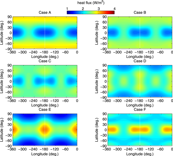
Figure 1. Surface heat flux (W m−2) distribution due to solid tidal heating for several cases with various partitions of activity between Io's mantle and asthenosphere. Case A: mantle dominated with polar maxima. Cases B and C: transitional, with  raised and
  lowered to gradually attenuate the mantle response. Case D: asthenosphere dominated, with six near-equatorial maxima. Cases A and D closely match patterns in Segatz et al. (1988), but here all of Cases A–F are adjusted to match a baseline total global output of 2.25 W m−2. Case E: a very low viscosity asthenosphere with high (465 km) thickness, leads to further equatorial focusing of heat. Case F: demonstration of how asthenosphere thicknesses beyond the expected range (here 700 km) does lead to further pattern variations. Note how in transitional cases (B, C) the relative difference between maxima and minima decreases, and the patterns achieve transition by first flattening out. See text for full case parameter details.
Download figure:
Standard image High-resolution image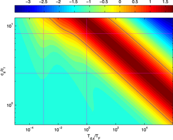
Figure 2. Solid tidal dissipative heat flux (Log10 scale with a basis of 1 W m−2) shown as a function of  (ratio of dissipation timescale to tidal period) and c/cr (where c is proportional to the square-root of the asthenospheric layer thickness h, and cr is the equatorial rotation speed). These coordinates are chosen for comparisons with the fluid-tide case and are given here a subscript "s" to distinguish them. The lower and upper horizontal lines (magenta) correspond to the assumption h = 20 km and h = 500 km, respectively. Vertical lines correspond to viscosities of
  and
and  Pa s. The solid curve (blue) corresponds to the value matching the observed heat flux, taken here to be 2.25 W m−2. The mantle viscosity is assumed to be
  Pa s, and the mantle and asthenosphere rigidity is
  1010 Pa m4. Simultaneous weakening of the shear modulus along with viscosity during melting, although not included in this figure, is found not to alter the figure's morphology. The system is insensitive to the core size of 350 km and lithosphere thickness of 20 km.
Download figure:
Standard image High-resolution image
Figure 3. Radial dependence of solid body tidal heating in Io, for the range of cases from Figure 1, with gradually increasing dissipation in a low-viscosity asthenosphere. Peak heating for the near-homogenous structure of Case A occurs mid-layer. When a low viscosity upper layer is introduced, peak heating occurs discontinuously at the asthenosphere-mantle interface. Heating due to tangential shear stress components dominates for the mid-layer peak of Case A, leading to polar maxima in surface heat flux. As any high dissipation top layer is expanded throughout the body (e.g., Case F), the form of the solution begins to return to the homogeneous solution. We consider Case B a primary candidate to blend with fluid tidal heating, in order to supply heat for polar volcanoes, yet still contain a modest asthenosphere. Heat rates are shown in W/m to eliminate the effect of the increasing volume of material at higher radii.
Download figure:
Standard image High-resolution imageIn all modeled cases, the lithosphere thickness is 20 km, core radius 350 km, and lithosphere viscosity 1022 Pa s. These values are maintained in all cases because the solution is minimally sensitive to their variation. A 50 km thick zone below the lithosphere is included to provide space for a "magma ocean" or magma slush layer of some form to exist. For the purpose of modeling the solid behavior in lower layers, it is only important that such a layer exists to mechanically decouple the lithosphere, and to demonstrate that we do not rely upon additional solid body heating from this volume to reach specific target values. This zone is modeled in our propagator solution code as a weak solid using a very low viscosity and shear modulus. This method was verified to closely match surface Love numbers obtained for a solution using the additional boundary conditions for a full liquid layer solution. The solid solution below this magma ocean is not sensitive to the choice of 50 km thickness, and solutions are nearly identical using such magma-accommodation layers with for example 1, 5, 10, or 100 km.
All silicate shear moduli also remain fixed at 5 × 10¹⁰ Pa. While solutions are more sensitive to this selection, we chose to isolate the role of viscosity and thickness variations here for clarity due to the large number of loosely constrained parameters in a multilayer system. The value  Pa is appropriate for solid silicate material; however, above the solidus temperature in particular this value decreases in the partial melt regime before becoming zero above temperature at which solid grains lose physical contact with one another (known as the break-down temperature). Therefore we emphasize that the 2.25 W m−2 dissipation level may also be achieved by cases involving decreases in the shear modulus, and the extreme low viscosity assumptions are not then required.
Solid Cases A–D overall represent a transition from a mantle dominated heating pattern (A), to an asthenosphere dominated pattern (D), with Cases E and F representing results for asthenospheres with higher thicknesses. In Solid Case A we use a mantle viscosity  Pa s, an asthenospheric viscosity
  Pa s, and an asthenospheric thickness tath = 200 km. Cases with closer-matched viscosities between the two layers lead to similar results, as Case A represents the solution of a near-homogeneous or homogeneous planet. In Solid Case B,
  = 1.215 × 10¹⁵ Pa s,
  = 1.5 × 10¹⁴ Pa s, and again tath = 200 km. In general for solid silicates at this forcing period, decreasing the viscosity will increase dissipation. In Solid Case C, the asthenosphere viscosity may be further lowered in order to further the transition to asthenosphere dominance, with values of
  = 1 × 10¹⁵ Pa s,
  = 6 × 10¹³ Pa s, and tath = 200 km. With numerous parameters across many layers involved in each solution, there are many alternative ways to achieve a given total heating rate and a specific pattern, and in particular asthenosphere dominance may be driven either by lowing the layer viscosity or by increasing the layer thickness. As an example, Case C may also be achieved using
  ,
,  = 1 × 10¹⁴ Pa s, and tath = 251 km. Solid Case D represents the classical asthenosphere-dominated six-maxima pattern described by previous works (e.g., Segatz et al. 1988). To reach the 2.25 W m−2 total heat flux rate with this pattern, we invoke
  = 2 × 10¹⁵ Pa s,
  = 1 × 10¹⁴ Pa s, and tath = 385 km. In general the viscosities used in these cases are low, and the asthenosphere thicknesses are high, as discussed in detail below. In agreement with the fully general solution range reported by Beuthe (2013), in Solid Cases E and F, we demonstrate that Case D is not a true end-member of the range of surface heat flux patterns possible for Io. We find that Case D has been concluded to be an end-member previously only because it is characteristically associated with asthenospheres of a specific moderate depth. The full range of surface heat flux patterns achievable due to solid dissipation is better characterized as a cycle, driven by the thickness of any upper high-dissipation layer akin to an asthenosphere. In the general solution, this upper layer may be another material such as ice, or a low viscosity silicate, and the total system behaviors is independent of the total planet size. Patterns such as Case A are characteristic of a homogeneous or near-homogeneous planet, where the peak in solid tidal heating with depth occurs in the center of the primary layer. Patterns such as Case D, E, and F are characteristic of situations where a high dissipation upper layer exists, and peak tidal heating occurs as a sharp spike at the layer interface. The cause of the final patterns is a complex result of blending the weighted sum of the tensor products for normal and shear stresses at each location throughout a body. A full discussion of this behavior is beyond the scope of this paper, but is treated to some degree (Henning & Hurford 2014). A simple understanding of the range of patterns is that shear stress terms, which lead to greater polar heating, dominate for situations such as Case A, and structures such as Case D involve a more even blend of shear and normal stress contributions.
Solid Case E uses  = 1 × 10¹⁶ Pa s,
  = 1 × 10¹⁴ Pa s, and tath = 465 km, while Solid Case F uses
  = 1 × 10¹⁷ Pa s,
  = 2.2 × 10¹⁴ Pa s, and tath = 700 km. Case E is likely near the limit of realistic asthenosphere depths possible for Io, and is interesting for the increased equatorial focusing of heat compared to Cases A–D. The 700 km asthenosphere thickness of Case F is unlikely to be realistic, and is presented here to demonstrate how the physical system continues through a further range. The pattern in Case F is nearly the exact inverse of Case B. Similarly, as tath is increased further the full cycle of solid tidal solutions includes cases that are the exact inverse of Case A and Case D, however the material layer structures leading to these solutions are often unrealistic. Figure 3 shows how these Cases fit together as part of a cycle. As asthenosphere depth is increased to high values, eventually this layer must consume the entire volume of the planet, and the solution must return to the homogeneous case. Case F begins to show this behavior, as a mid-layer peak in heating re-emerges when the weaker top layer reaches approximately half of the total solid radius.
A material viscosity of 1013 Pa s is low for silicates, particularly in comparison to values such as 1020–1024 Pa s expected for Earth's mantle (Mitrovica & Forte 2004). Silicate viscosities in the 1012–1015 Pa s range are however commensurate with values achieved by the melting parameterizations of Moore (2003) and Fischer & Spohn (1990), following experimental data by Berckhemer et al. (1982), for temperatures at or near the solidus, as well as the bulk viscosity of silicate partial melts in the 0%–40% melt fraction range. Therefore the values tested here are compatible with a possible deep system of partial melt veins, heat pipes, and native solid rock at, or just, above the solidus temperature.
Asthenosphere thicknesses of 200–500 km are high compared to values of 50–100 km often considered for Io, however, Moore (2001) demonstrates that it is reasonable for melt production and transport to be occurring in a 500 km thick layer on Io. Moore (2001) also shows that Io is likely to contain a gradual continuum of melt fractions varying with depth, making it difficult to declare where the layer boundary for an asthenosphere based on viscosity will exist. We have performed some simulations of systems with high numbers of solid layers, including continuum gradations of viscosity with depth. Such models show that total solid dissipation is strongly controlled by the lowest-viscosity uppermost layer, and therefore solutions such as Cases A–F change only moderately when gradations are introduced below the asthenosphere-mantle boundary. A full discussion of such parameter gradations is beyond the scope of this paper and is the subject of ongoing work.
In Section 4, we discuss the relative fraction of the total expected parameter space for solid body heating that does or does not fulfill the observational requirement of approximately 2.25 W m−2 in global tidal heat output. In general, while solutions such as Cases A–F that satisfy this heat level are possible, there is a much wider range of solid body solutions that fall far short of the observed total heat. This key feature of the solid body tidal heating physics for Io is strong motivation to consider fluid layer tidal heating as an additional source of energy. Note that it is possible to achieve the patterns shown in Figure 1 for a wide range of total heat magnitudes, because the patterns are primarily a result of the layer thicknesses and ratios of layer viscosities, and not a function of the absolute value of viscosities themselves.
In all solid heating cases heat generation is symmetric about the subjovian point, and thus unable to explain any systematic longitudinal offset of volcanism (e.g., Kirchoff et al. 2011; Veeder et al. 2012; Hamilton et al. 2013) without further invoking convection asymmetries and/or crustal inhomogeneities that may have been imprinted in Io's geological history.
3.2. Tidal Dissipation in the Fluid
In Figure 4, we show the rate of work performed by the temporally fluctuating (tidal) gravitational field of Jupiter as projected onto a globally extending fluid layer of uniform thickness (h), located near the surface of Io. The tidal work here represents the average over the globe and over a tidal cycle, and is equivalent to a similar temporal and spatial average of the tidal dissipation. The equivalence of the integrals of work and dissipation in solid tidal models is the result of total energy conservation, together with the assumption that an equilibrium has been reached. But in the case of fluid tidal heating, this equivalence is not required locally because there are also advective fluxes of energy within a fluid system. We furthermore assume that the total tidal dissipation is equivalent to the rate of heat production and that this is presented at the surface as a heat flux. While these additional assumptions are not required in discussing the global tidal response solutions calculated, the translation to surface heat flux values is included to ease the discussion and reference to observations.
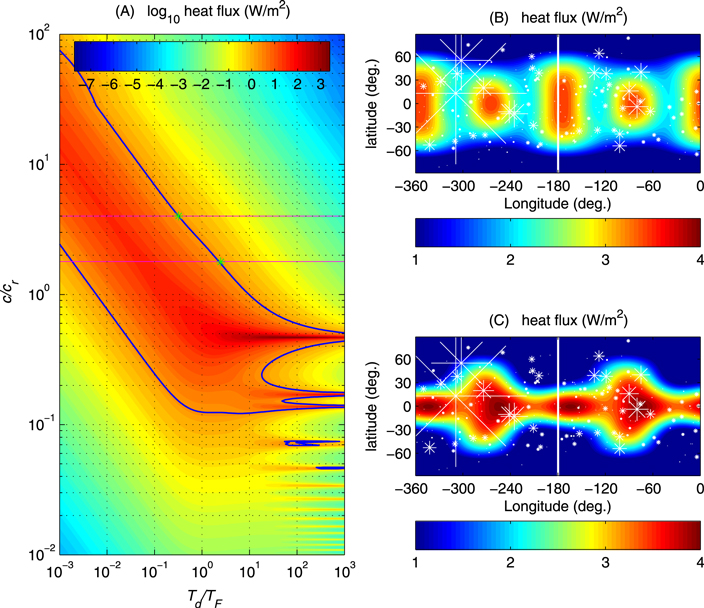
Figure 4. Left panel (A): Fluid tidal dissipative heat flux (Log10 scale with a basis of 1 W m−2) shown as a function of the unknown parameters  (the dimensionless dissipation timescale) and c/cr (the dimensionless dynamical wave speed which depends on the fluid layer thickness h). The lower and upper horizontal lines (magenta) correspond to the assumption h = 10 km and h = 50 km, respectively. The solid curve (blue) corresponds to the value matching the observed heat flux, taken here to be 2.25 W m−2. The upper and lower astrices describe end-member scenarios for which the associated spatial distributions of the heat flux are shown in the respective upper and lower right panels (B) and (C). Stars in the right panels show the locations of dark floored paterae from Veeder et al. (2012), with symbol sizes scaled to their power output.
Download figure:
Standard image High-resolution imageThe left panel (A) in Figure 4 shows a solution-space diagram in which 70,000 tidal response solutions are calculated to provide the average "heat flux" as a function of two unknown parameter coordinates  and
and  :
:
The parameter Td is the timescale for momentum loss from the fluid layer. As described in the  , which is the ratio between the forcing and attenuation frequencies. The parameter represented by the ratio
  , where TF is the forcing (tidal) period, is then a non-dimensional timescale associated with the dissipation and is related to the familiar "quality factor" Q. But use of Q as a fundamental parameter is avoided here because of potential confusion stemming from, among other things, the fact that Q often does not have a unique definition in problems where there can be multiple definitions of the system energy. In the case here, it is an arbitrary choice of whether potential energy should be included as part of the system energy. And if it is included a further choice is whether it should be defined with respect to the time-varying or time-averaged geopotential.
The parameter c is the wave speed (unknown) appropriate for the fluid, and cr is the equatorial rotation speed (74.9 m s−1). The parameter represented by the ratio  is then a non-dimensional wave speed describing how well the dynamical adjustments in the fluid can keep up with the phase propagation of the forcing. In the standard shallow-water relationship (assumed here),
  and therefore c depends on the gravitational acceleration g (1.80 m s−2) and the thickness h (unknown) of the fluid layer. In this initial study, no attempt is made to examine potentially appropriate modifications to this simple relationship to include stratification, effects associated with multiple phases in the fluid, or effects due to mass-loading or flexure of the crustal layer above. It is expected that some of these additional effects can be included as shifts in the effective values of
  and
and  , which in either case remain only loosely constrained.
The "picket fence" of features in the lower right of Figure 4 (A) describes the resonant excitation of a primary mode by the degree-2 tidal force, and the scattering of this energy through harmonic components due to Io's global rotation. These resonances survive only in the weakly damped situation, which we do not expect for the flow of a partial-melt magma where it should be expected that there is strongly effective viscous and form drag. The broad peak seen across the left of the diagram is probably not best described as due to a resonance because for these parameter values the hyperbolic (wave-like) governing equations have approximately merged with parabolic (diffusive) forms describing creeping flow (see  is simply equal to twice Q (under the definitions described in the
The solution-space (Figure 4(A)) provides a generic description of the dependence of the heating rate on the nondimensional timescale for dissipation and the propagation speed associated with a primary uncoupled wave speed in the fluid layer. But this large generic parameter space can be constrained by both observations and specifications of physical processes.
Results in Khurana et al. (2011) demonstrate that Io has at least 20% melt over a thickness of at least 50 km. We take this as a soft constraint on h from which we assign h = 10 km and h = 50 km as the expected minimum and maximum values. This assumes that we can safely collapse a partial melt layer into the equivalent thickness of a pure fluid layer for purposes of the computation of tidal work. These limits on h are transposed to limits on the wave speed ratio coordinate  in Figure 4, under the simple shallow-water assumption described above, and the solution is then constrained to fall between the horizontal (magenta) lines included in the diagram. The observed heat flux, taken here to be 2.25 W m−2, or equivalently a global total of 93.8 terawatts (TW; Lainey et al. 2009), provides another constraint, requiring that the solution fall on or exterior to the solid (blue) curve shown. The solution must, however, remain close to the contour if we restrict our attention to solutions that contribute a significant fraction of the observed heat.
From these constraints, two end-member solution scenarios are selected (shown by green astrices). The parameter coordinates are ( = 0.32,
  = 4.0) and (
 = 2.4,
  = 1.8), which correspond to the dimensional coordinates (Td = 17 hr, h = 10 km) and (Td = 2.2 hr, h = 50 km), where the dimensional dissipation timescale Td may be interpreted as the amount of time required for the fluid to come to rest if tidal forcing were suddenly turned off. It would be very useful if an independent constraint on Td could be estimated. Our attempt toward this has not been helpful, however, because of the large range of viscosity values possible and the uncertainties on how best to parameterize form drag for this case. We may note, however, that the range (
 0.32–2.4) meeting the other constraints does not appear to be unreasonable. Interestingly, this range also straddles the value
  (Q = 0.5), describing the critically damped situation in which restoration of equilibrium is most efficient and may be the result of feedbacks.
The result we have described above in this section pertains only to the total (or average) tidal heat associated with a wide range of potential parameter scenarios. In this case only one number represents each scenario. Of course there are further aspects to the tidal response solution, some of which may be used for further comparisons with observations, or to provide distinguishing features of the fluid response that may be used in future tests to separate fluid and solid responses. A distinguishing element of the fluid response which also has an observational basis for comparisons is the spatial distribution of the heat generated. We provide here examples (Figure 4, right panels) corresponding to the end-member scenarios shown by the green astrices in (left panel). Solutions between these two scenarios (and following the blue curve) show a gradual focusing of heat generation toward the equator as  (thereby h) is decreased, and an asymmetric shift along longitude becomes more pronounced. This shift will be further discussed in Section 4.
4. DISCUSSION
The results of this study show that either solid-body tidal dissipation or fluid tidal dissipation can account for Io's observed surface heat flux; however, it is also possible that both of these processes operate simultaneously. In this section, we first examine the implications of each of these mechanisms operating independently and then consider scenarios in which they combine together.
4.1. Solid Tidal Dissipation Only
Let us first demonstrate that for some restricted set of parameter choices, solid tidal dissipation acting alone can supply the average Ionian heat flux, taken here to be nominally 2.25 W m−2. Figure 2 shows a parameter space of solutions for the solid tidal dissipation for Io. The coordinates are derived from the two most important controlling parameters for the solid,  (material viscosity) and h = tath (asthenosphere thickness) and are intended to facilitate comparison with the solutions for fluid tides in Figure 4. For the abscissa, we generate a damping timescale Td from the material viscosity
  assuming Td =
  , where ρ is the material density (taken here to be 3500 kg m−3), and A is the surface area involved in viscous action, in this case the constant top area of the asthenosphere. Note that a subscript "s" refers to "solid" and is attached to emphasize that the parameters cs and
  have a necessarily different basis of formulation in the solid and fluid cases. The axis
  is constructed from h just as in the fluid case, but one should note that the interpretation of h in the fluid case was that h represents only the fluid fraction of the asthenosphere. Hence, the potential range for h in the fluid case used a smaller expected upper value than in the solid case here. Mantle viscosity is assumed to be 1017 Pa s, keeping mantle tidal contributions very low. High mantle dissipation leads to a plateau in the heating rate across the lower left corner of the Figure where asthenosphere activity otherwise tapers off. Note that this Figure models only dependence on viscosity for the purpose of comparison with the fluid, and does not include the impact of melting and the loss of shear strength that occurs generally for silicate systems much below η = 1012 Pa s. Thus in practice, to understand low viscosity behavior, it is necessary to switch to the fluid solution.
By this same scaling of Td, the 5 hr damping timescale of the preferred solution from Figure 4 translates to a fluid system effective viscosity of ∼7 × 10¹² Pa s. However, this effective viscosity it is not straightforward to assess because it would result from a combination of form drag, material viscosity, and boundary-layer friction. The material viscosity of magmas is generally in the range from 1 to 100 Pa s, but it may not be unreasonable for such a fluid shifting within a solid matrix at tidal frequencies to achieve the effective interphase value above.
Figure 2 shows that the space of solutions includes solutions (lying on the blue curve) producing the observed 2.25 W m−2. A subset of these solutions also fall within the expected range for h (20–500 km) shown by the horizontal (magenta) lines. A significantly smaller subset of these also fall within the range for the expected material viscosity (1012–1015 Pa s), shown by the vertical (magenta) lines. In short, solid tidal solutions produce the observed heat flux but only for a very restricted range of the potential parameter combinations.
Viscoelastic solid systems are well known (e.g., Nowick & Berry 1972) to exhibit a form of material resonance (even with inertial terms neglected), whereby there is a forcing frequency or equivalently a temperature or pairing of viscosity and shear modulus, at which maximum viscoelastic response occurs. This behavior is evident in any horizontal cross-section of Figure 2. While one might expect that the global total of solid tidal heating would simply increase with increasing thickness of the active layer, we find that the solid system is also able to cross the apparent resonance band in the response by changing h alone (where h in this context is the same as tath). This occurs due to the focusing of stress at the bottom of the asthenosphere layer, which rises sharply as the resonance thickness is crossed, but which is also convolved with the changing volume of material in tidal action as h varies. This behavior may partly be seen in Figure 3, although viscosity is not held constant in these cases. A modest number of calculation steps (15–20) through such layers are necessary to resolve this behavior. Very weak branching bands also exist in Figure 2 due to similar inter-layer changes in the relative magnitude of stress concentrations (e.g., in the middle left of the phase space) but these features are too faint to control the global tidal behavior.
Figure 2 highlights the similarities of the solid and fluid analytical solutions. Both lead to a primary band of elevated heat flux controlled by the layer thickness and damping, with similar orientation and magnitude of variation. The solid solution resembles the creeping flow limit of the fluid solution, but lacks the "picket fence" of finer fluid resonances at lower thicknesses. A key difference occurs where the expected solution for Io is placed relative to the resonance band.
In the solid case, the expected range of parameters (roughly  = 1012–1015 Pa s, and tath = 20–500 km) places the result in the mid-upper left of the figure, but below the resonance band, including only part of the lower shoulder of the band. The peak dissipation rate of the band is somewhat beyond the expected tidal heating range. This explains the idea that solid dissipation, while capable of generating the observed tidal heat rate of Io, only achieves this rate of activity in a small corner of the expected parameter space, while the majority of the expected solid solutions lead to insufficient heat. If only
  and tath are considered, this location of the solid solution would seem subject to unstable feedback: higher tidal activity would increase partial melt, shifting the system to lower viscosity and higher h, up the shoulder of the resonance band toward greater dissipation. Less heating would lead to runaway cooling. These behaviors are, however, interrupted by feedback with convective cooling (Moore 2001), which leads instead to stable solid tidal-convective equilibria at modest melt fractions.
Regarding the global distribution of the heat flux, the solid tides appear unable to produce the longitudinal offset inferred from observations. The mathematical reason for this is discussed in Section 4.4.1.
4.2. Fluid Tidal Dissipation Only
Figure 4 illustrates that a global magma ocean treated as a fluid subject to the Laplace Tidal Equations also produces the observed average heat flux for a subset of the parameter coordinates (blue curve). If, as expected, the fluid is overdamped (i.e.,  ), then the solutions to these complete equations converge with solutions obtained for a simpler set of equations describing creeping flow (see
  ), rotational/inertial aspects of the fluid behavior differing from the solid case are present even in the overdamped case.
Regarding the global distribution of the heat flux, the fluid tides are generally not symmetric with respect to the antijovian meridian because rotation causes the propagation speed of fluid adjustments to depend on whether the propagation is eastward or westward. Solutions are included (e.g., the low-h example in Figure 4), which can explain the observed offset and also agree with other constraints. In summary, the fluid tides, even if acting alone, can provide solutions in agreement with the observed heat flux amplitude as well as the meridional offset of the distribution, and unlike solid-tidal dissipation, may do so over a relatively broad span of their plausible parameter space.
A feature of the full set of the solutions shown in Figure 4, is that eccentricity driven tides are focused at the equator and therefore there is reduced ability in explaining inferred heat fluxes near the poles. However, in the case of obliquity driven tidal forces, the fluid tidal response is focused at the poles rather than the equator. Although the heat fluxes associated with the obliquity tides have also been calculated and studied in this research, they have not been presented here as the amplitudes are too small to be significant. The latter calculations assume only the very small value for the obliquity of 0 05 consistent with a Cassini state following Bills (2005). It is possible that a higher obliquity (possibly in episodes) together with the observed eccentricity create a fluid tidal dissipative heat flux in agreement with both the equatorial and polar distribution of heat fluxes inferred from observations. But for the present eccentricity and expected Cassini-state obliquity, fluid tides do not readily account for the distribution of heat flux at high latitudes.
4.3. Consideration of Feedbacks Promoting Simultaneous Solid and Fluid Tidal Dissipation
We now discuss the potential coexistence of both solid and fluid tidal heating at significant levels. While there may be the somewhat singular case where both processes simply happen to provide comparable heat levels, we note that this coincidental match seems unlikely given the large potential ranges of each. Of interest here is to decide whether one process may promote the other such that both occur simultaneously at significant levels.
The stability in time of individual parameter states may first be addressed using the parameter-space solutions for either the solid in Figure 2, or fluid in Figure 4. These Figures compactly describe heat fluxes associated with various parameter coordinates, but are also useful for estimating which parameter coordinates are stable against perturbations in the layer thickness (h). While these parameter spaces describe solutions that are consistent with equations, many parameter coordinates are unstable configurations in time due to feedbacks. First consider solid-body solutions that fall on the lower-h side of the elevated heating ridge in Figure 2. A perturbation increasing the asthenospheric thickness h then leads to higher heating rates, or equivalently higher heating will lead to more magma production and a larger h. This is an unstable feedback, which is ultimately only halted by a separate process involving convective cooling. Stable points in Figure 2 reside on the upper side of the heating ridge rather than the lower side, where increasing h will decrease solid-body heating. The same feedback applied to fluid tides shows that candidate solutions discussed in the fluid case are stable when they fall on the upper side of the ridge in Figure 4.
In one example, coexistence of solid and fluid layers in some form is favored whenever solid-body tidal heating is significant enough to produce magma. Solid tides are well known to exhibit feedback with convective cooling (Moore 2003) which typically regulates their incidence to a mid-valued melt fraction when a layer is considered in aggregate. Moore (2003) predicts this equilibrium melt fraction to be in the range of 40%–60%, near the material breakdown temperature. Even if a given layer is cooled by advective transport of heat upwards by heat pipes and melt separation, the same feedback exists, as cooling becomes more vigorous with increasing melt availability. The fact that solid-body tidal activity naturally evolves to such a melt fraction range, the same range where fluid and solid activity are both likely to have similar heat rate magnitudes, greatly elevates the probability of simultaneous occurrence above a purely random pair of solutions from each space of solutions.
Given tidal forcing as strong as at Io, there are only two pathways to eliminate solid-body tidal heating: first by the body becoming too hot, and second by becoming too cold. Peale et al. (1979) found that global effective silicate viscosities in the warm range of partial melting (e.g., 1012–1016 Pa s) are needed to explain Io's tidal heating via solid friction. However, if the cool (or high pressure) viscosity range typical of Earth's upper mantle, 1019–1023 Pa s (Mitrovica & Forte 2004) is applied to Io, the result is negligible solid heating. The hot pathway includes co-existence of solid and fluid layers, and occurs through a thermal runaway, whereby a large fraction of the mantle is converted into melt, such that the bulk material viscoelastically decouples from its material resonance with the forcing frequency (Peale et al. 1979). There are two arguments against this behavior driving present conditions on Io. First, convective cooling prevents this runaway process from occurring in full, and leads instead to equilibrium at a modest melt fraction. Second, even if runaway melting could occur, it leads to high thickness liquid layers that are not favorable to fluid-body tidal dissipation and subsequent replacement of the solid-tide heat source. Therefore elimination of solid-body tidal activity via this hot pathway is implausible.
Any cold pathway to eliminating solid-body tidal heating but still preserving fluid heating presents challenges. It is impossible in thermal equilibrium to have a hot magma layer above a colder layer. The weak role of pressure on Io also makes the rise in the melting (solidus) temperature with depth quite gradual. Thus material directly below any magma layer on Io would be at nearly the same temperature and pressure, and therefore within the regime of near-solidus viscosities where solid-body tides are strongest. The shallow rise in solidus temperature with depth will also mean that this near-solidus state would remain true over a significant thickness, even if temperature rose no higher all the way to Io's core. Given that a 100% melt fraction layer is unlikely to begin with, more likely is a gradual transition in depth of a magma-slush partial melt layer into near-solidus material below. Again, such a configuration meets both the criterion of coexistence of fluid and solid material, as well as solid material in the near-solidus and partial melt viscosity range where solid-body heating is strongest. Only the volume of solid material in the appropriate viscosity range remains in question, and most melt transport and percolation models (Spiegelman 1993; Moore 2001) favor a high transition zone thickness commensurate with the 200–500 km needed for significant solid-body tides. The only plausible mechanism to have a high melt fraction magma layer immediately underlain by solid material at very high viscosity is for a radical change in composition. Therefore most cold pathways to eliminating significant solid-body tidal heating also require cooling the moon so far as to also eliminate fluid layers. Clearly eliminating both sources of heat would fail to match observations.
Next, consider interactions between solid and fluid processes over Io's history. Any fluid within Io must have an origin. Fluid may either persist since Io's formation, or be produced by later melting of solid material. At one extreme, consider a case where solid tidal heating is fully absent, perhaps due to a very high (cool interior) solid viscosity. Very low solid-body tidal heating would be expected to result in near zero magma, thus near zero fluid heating, analogous to Earth's inactive moon today. Any fluid heating occurring without present day solid-body heating on Io would therefore be required to have remained fully self-sustaining, without any interruption, since just after the formation of Io, or alternatively would still require an episode of solid tidal heating in the more recent past as a trigger. A model whereby Io's present magma ocean is a small remnant of a largely fluid interior that has been crystalizing gradually over solar system history is untenable, as fluid-body tidal heating is only efficient for thin layers, and therefore any high fluid-volume initial conditions 4.5 Gyr ago will rapidly crystalize back to a mostly solid body, with a thin (efficient for fluid tides) magma layer. A glancing impact and the resulting obliquity and spin interruption could provide a recent trigger. Evidence for such impacts on Io are however rapidly erased given Io's high global resurfacing rate, and surface age of ∼1 million years (McEwen et al. 2000, 2004).
Fluid heating has the property that once it has begun to occur at a significant rate, it prevents the freezing out of the layer involved, since thinner layers lead to greater heating, and this feedback can stabilize the activity at an equilibrium rate. While thin fluid layers do promote the endurance of fluid tidal activity through this feedback, their very small fluid-layer volume is highly vulnerable to freeze-out if orbital oscillations cause any era of decreased tidal forcing. A thin layer of only a few kilometers, linked to the surface by magma heat pipes, is liable to crystalize in only a few million years if its tidal impetus is temporarily removed. This issue leaves little room for error in attempting to sustain fluid tidal heating within Io for all of solar system history, without the assistance of solid-body tidal heating as a way to replace magma. A fluid-only model therefore prefers steady orbital forcing, and fluid heating may have difficulty restarting after lower eccentricity excursions in the widely oscillating orbital behavior of the Galilean Laplace system (e.g., Fischer & Spohn 1990; Hussmann & Spohn 2004). In contrast, solid tides have the ability to restart after eccentricity is restored. The fact that fluid tides are not robust against low eccentricity orbital variations over the past 4.5 Gyr, causes a strong preference for models where solid and fluid tidal activity occur together. The arguments here ignore obliquity driven tides and some reconsideration is required if Io is allowed much larger obiquity values than the present.
Lastly, we ask whether or not fluid tidal heating may cause the known process of tidal-convective equilibrium described above to become unworkable. For a case of Io in solid-body-tidal-convective equilibrium, all that is required for the system not to evolve out of such a range is that subsequently occurring fluid heating is not so great as to carry the system on a runaway to a 100% melt fraction. But such a runaway for the fluid system cannot occur, because evolving to a greater thickness of even hotter material would mean moving within Figure 4(A), upwards and to the right of any prior solution (e.g., the preferred solutions marked). This, however, would decrease the fluid heat output. Thus both the solid-convective and fluid tidal behaviors regulate the system away from complete thermal runaway, and fluid-body tidal heating does not perturb out of existence the tidal-convective equilibrium described by previous authors. Instead, fluid tides will merely shift the convective-equilibrium temperature (and thus melt fraction) to a slightly higher value. One may imagine a fluid-body tidal heating peak superimposed upon Figure 1 of Moore (2003), between the solidus and breakdown temperatures. Linear summation of such a new fluid heat source peak with the peak for solid-body tides would thus shift the total-tide-versus-convection equilibrium intersection to a higher temperature, with the magnitude of shift depending on the unknown fluid dissipation rate. In theory, a dual peak of both solid and fluid tides could lead to a pair of stable tidal-convective equilibria, akin to the dual-peak states described in Henning et al. (2009) for the Burgers rheology. In practice however we find that few plausible parameter cases separate the maxima temperatures of the two processes far enough for this to occur. Therefore adding fluid-body tidal heating to Io maintains the mechanism of tidal-convective (or tidal-advective) equilibrium, and will lead to equilibria at a modestly higher temperature and higher melt fraction, determined by the magnitude of the fluid dissipation term.
We therefore find numerous feedback mechanisms and coexistence arguments that favor the simultaneous production of similar levels of solid and fluid tidal heating within Io. The simplest summary of this conclusion comes from the very notion that a partial melt layer, gradually decreasing in melt fraction with depth, is by its very nature an ideal environment for both sources of heat, with fluid heating favored in upper high-melt fraction levels, and solid-body tidal heating favored in lower low-melt fraction levels. The dimensions (200–500 km), temperatures, and melt fractions (∼0%–50%) of such a region are commensurate with the high heat rate solutions for both processes. Feedback between both tidal inputs and convective (or advective) cooling will also strongly drive Io to a stable temperature equilibrium at just such a global state. Stable equilibrium in the thickness of such a layer is also favored by both processes, with no tendency for unstable runaway of asthenosphere thickness to either 0 km or RIo. Both fluid and solid heat sources favor the creation and continued existence of the other, while eliminating one heat source without eliminating both (via hot or cold extremes) is very difficult to achieve.
4.4. Comparison Between Model Predictions and Observations
4.4.1. Solid-body Tidal Dissipation
Solid-body tidal heating models can reasonably explain Io's total power output, but the predicted distributions of surface heat flux exhibit significant inconsistencies with the observed locations of volcanism. For instance, if tidal heating dominantly occurs within the deep-mantle, then the overall pattern of heat flux at the surface is expected to have maxima near the poles and be relatively low near the equator (Figure 1). Assuming that volcanism is correlated with expected surface heat flux, this result is inconsistent with observed concentrations of volcanic centers on Io at low-latitudes (Lopes et al. 2004; Williams et al. 2011a, 2011b). Solid-body tidal heating within the asthenosphere offers an improvement, in that these models predict enhanced heat flux near the equator with a spherical-harmonic degree-2 pattern centered along the tidal axis (Figure 1). This prediction generally agrees with the results of spherical harmonic analysis applied to the distribution of mountains and volcanic centers on Io in that they exhibit statistically significant power at degree-2, with concentrations in spatial density at low latitudes (Kirchoff et al. 2011). This result implies an important role for tidal heating within the asthenosphere, but these solid-body models fail to account for observed asymmetry in mountain and volcano concentrations relative to the tidal axis (Kirchoff et al. 2011; Veeder et al. 2012; Hamilton et al. 2013). Additionally, major volcanic systems on Io such as Loki Patera (13°N, 309°W), are located in relative minima in the near-equatorial surface heat flux pattern predicted by solid-body tidal dissipation in the asthenosphere. Loki Patera is often treated as an anomaly among Io's 133 dark floored patera because it covers only 0.07% of Io's surface area yet accounts for 10%–20% of Io's total heat flow (Veeder et al. 1994). However, other major volcanoes such as Tvashtar (64°N 128°W), Dazhbog (55°N 302°W), Thor (39°N, 124°W), Amerasu (38°N, 307°W), Daedalus (20°N 307°W), Creidne (53°S, 342°W), and Catha (54°S, 102°W) paterae (Lopes et al. 2004), together accounting for nearly a quarter of Io's total power output (Veeder et al. 2012), are also poorly reconciled with conventional model predictions. These discrepancies provide a strong indication that the conventional solid-body tidal dissipation models provide an incomplete description of Io's internal heating mechanisms.
Note that the symmetry in maps of solid-body tidal heating about the subjoin point arises mathematically due to the simple cosine symmetry of the disturbing potential function in longitude when at pericenter or apocenter, combined with the fact that dissipation, always positive for both positive and negative potential excursions, is equal in magnitude across the surface for a given mean anomaly ahead and behind pericenter. Therefore the orbital integral of ideal solid heating is always symmetric.
4.4.2. Fluid-body Tidal Dissipation
Dissipation of tidal energy within fluids in Io's asthenosphere provides an alternative to the classical solid-body tidal heating approach. Figure 4 provides examples of expected surface heat flux patterns for an asthenosphere in two regimes that could account for global power output for Io. In the creeping flow regime, patterns of predicted surface heat flux resemble those for the asthenosphere-dominated solid-body dissipation cases shown in Figure 1, with the same strengths and weakness in terms of matching observed distributions of surface features. However, in the more fluidal case, there are differences that dramatically improve the fit between predicted surface heat flux patterns and the observed distribution of mountains and volcanism. The overall pattern of surface heat flux in the more fluidal case still shows a near-equatorial concentration, but the degree-2 maxima are located closer to the centers of the trailing and leading hemispheres. Secondary maxima are also located ∼30° to the east of the tidal axis. This pattern of expected surface heat flux provides a much better agreement with the calculated locations of volcano clusters on Io (Kirchoff et al. 2011; Veeder et al. 2012; Hamilton et al. 2013) and the observed distribution of major volcanoes including Loki Patera. For example, among the fourteen largest volcanoes on Io, which account for nearly two-thirds of the global power output, all but Tvashtar and Catha paterae show a close spatial association with regions of enhanced surface heat flux expected from fluid tidal dissipation in the asthenosphere. Nonetheless, there are many smaller volcanoes at high latitudes that are poorly described by this model, which raises the question: could both fluid-body tides in the asthenosphere and solid-body tides in the deeper mantle combine to produce the observed distribution of heat production and volcanism on Io?
4.4.3. Combined Fluid- and Solid-body Tidal Dissipation
Figure 6 provides an example of a combined case in which 50% of Io's total heat comes from fluid-tidal dissipation within a relatively fluid asthenosphere and 50% comes from solid-body dissipation in the deep-mantle (these source depths are shown schematically in Figure 5.) This combined model predicts enhanced heat production and melt generation at low to mid-latitudes, and is consistent with the observed concentration of volcanoes near the equator. Additionally, the thin asthenospheric layer of interconnected partial melt in this model could promote the interaction between the densely populated volcanic hotspots in this region. This is consistent with the observation by Hamilton et al. (2013) that hotspots in the near-equatorial third of Io appear self-organized into a repelled distribution and that volcanic systems in this region may tend toward a maximum packing arrangement due to a resource (i.e., magma) scavenging process. Additionally, the combined model exhibits an eastward offset in surface heat flux maxima relative to the tidal axis by the ∼30°, which provides excellent agreement with the location of Loki Patera and other major volcanoes (see discussion above for the relatively fluid asthenospheric case). The addition of a deep-mantle component in this combined model also extends the range of enhanced tidal heating further toward the poles, thereby helping to reconcile the location of Tvashtar Patera. Additionally, if melt feeding these high latitude volcanoes comes from a separate deeper-source, then the combined model may explain the observation that volcanoes at high latitudes (poleward of ±1947) exhibit a homogeneous Poisson (i.e., random) distribution, consistent with independent formation (Hamilton et al. 2013).

Figure 5. Sketch of a model for Io with simultaneous fluid and solid tidal heating occurring in separate layers, whereby both equatorial and polar volcanic sources receive adequate tidal heat input. In this model, fluid tidal heating originates from a thin magma ocean, asthenosphere, or magma-slush partial melt layer, and provides tidal heat flux primarily into equatorial volcanoes in a pattern that is not symmetric about the sub-Jovian point, but instead offset in longitude by approximately 30°. Simultaneous solid-body tidal heating occurs in this model below this high melt fraction top layer, and consistently with mantle-dominated solid-body tidal models, produces a significant polar contribution of tidal heat flux. If significant magma mixing did not occur, this model would predict that polar volcanoes may have observational evidence for being sourced from high depths (e.g., higher eruption temperatures), with equatorial volcanoes sourced from shallow depths. Black and white arrows represent heating from the deep mantle and asthenosphere, respectively, and are scaled to schematically represent the latitudinal variation in heat flux.
Download figure:
Standard image High-resolution image
Figure 6. Map of the tidal surface heat flux for a combined case that includes both fluid and solid tidal heating. In this model, both fluid and solid heating are for illustrative purposes made to generate equal contributions. A mantle-dominated solid-body tidal case is used to improve the contribution of heat to polar volcanoes. Note how the overall visual pattern remains dominated by the fluid-body pattern, due to the high maxima of the fluid case. Compared to the fluid case, the spread of heat flux magnitudes between the minimum and maximum values of the solid-body case is small, and therefore is adding solid-body tidal heat is akin to adding a significant but relatively uniform background heat flux rate onto the strongly varying fluid tidal heat pattern. Nonetheless, the combined model achieves the goal of supplying tidal heat to both the poles and equator, with equatorial maxima shifted ∼30° in longitude from the subjovian point. Stars in the right panels show the locations of dark floored paterae from Veeder et al. (2012), with symbol sizes scaled to their power output.
Download figure:
Standard image High-resolution image
In addition to the improved agreement between predicted surface heat flux patterns and the distribution of active volcanism, there are some improvements with respect to mountain distributions as well. Kirchoff et al. (2011) identified a statistically significant anti-correlation between the degree-2 pattern of volcano and mountain distributions on Io. Using a conventional asthenospheric-dominated model (e.g., Ross & Schubert 1985, 1986; Segatz et al. 1988; Tackley et al. 2001; Hamilton et al. 2013), concentrations in the distribution of mountains appear correlated with regions of enhanced heat flux near the subjovian and anti-Jovian points. However, an elevated geotherm in these regions would promote more rapid crustal subsidence and viscous relaxation of the mountains. In the combined model shown in Figure 6, regions ±30° poleward from subjovian and anti-Jovian points have much lower expected surface heat flux than in in the conventional model. This would favor a thicker and stronger crust in these regions, thereby helping to support Io's extremely tall mountains, which can reach up to 18 km in height (Schenk et al. 2001; Jaeger et al. 2003).
This example of a 50/50 combination of fluid- and solid-body tidal dissipation mechanisms does not consider the intricate feedbacks between these two processes discussed above, nor does it fully explain the location of mountains and volcanoes on Io, but it does identify a promising new direction in terms of considering the implications of high partial melt fractions within Io's magma ocean.
5. SUMMARY AND CONCLUSIONS
Io is perhaps the best example available for study of a planetary body under extreme tidal heating. The tidal response of Io is highly significant in the moon's internal dynamics and structure as well as its orbit and rotation. Study of this tidal response is of specific relevance to Io but is also clearly relevant to the general study of solar- and extra-solar planetary systems.
This study was motivated by several observations: (1) the tidal response of a fluid can be quite unlike that of solid; (2) Io is expected to have a partially fluid interior; and (3) all previous studies of Io's tides treated the body as essentially a solid. Previous estimates of the tidal response and associated heat generation on Io are incomplete and possibly erroneous because dynamical aspects of the fluid behavior are not permitted in the modeling approach. This study addresses this by modeling the fluid asthenosphere ("magma ocean") as a global layer of fluid governed by the Laplace Tidal Equations. Solutions for the fluid tidal response are then compared with solutions obtained following the solid-material approach. In each case, a family of solutions must be considered because of the imprecisely known parameters that must be assigned in the calculations.
In treating Io as a solid, it is found that the tidal heat generated can match that of the average observed heat flux (nominally 2.25 W m−2), though only over a very restricted set of parameters within the plausible range. Further, the distribution of the solid tidal heat flux cannot readily explain a longitudinal shift in the observed (inferred) low-latitude heat fluxes. Finally, consideration of a feedback in which tidal heat increases the thickness of the asthenosphere suggests that this reduced set of configurations that are consistent with the constraints, may not be stable with respect to perturbations of the parameters controlling the tidal solution. In treating the magma ocean on Io as a fluid, it is found that the observed average heat flux can be provided over a wider range of plausible parameters than in the solid case. A basic indication of this is seen by comparing the solution sets Figures 2 and 4. In the fluid case, magnetic observations provide the contraint that the solution fall within the horizontal lines indicated in Figure 4. Solutions for all but the underdamped regime ( corresponding to solutions where the tides dissipate on timescales longer than the forcing/rotation period) show heating rates at or exceeding that observed (blue line). Because underdamped solutions may be unlikely, it seems that plausible solutions from the model of the fluid tides all show significant heat generation. Such constraints implicating high expected heat are not available for the solid tidal case. The longitudinal offset in subsurface heat sources, which we take only as suggested in the observed surface heat distribution, can also be explained within fluid-tidal solutions using a further reduced set of parameters.
Finally, these candidate fluid-tide configurations appear to be stable with respect to perturbations in the controlling parameters (i.e., the configuration would not quickly migrate to one with new parameter values). These eccentricity-driven fluid tides are, however, focused at low latitudes and cannot readily account for heat fluxes inferred at high latitudes. Obliquity-driven fluid tides are indeed focused at the poles and may provide an explanation, but only if Io's obliquity is much higher than the very small forced component expected for a present Cassini state. A second possible scenario consistent with all observations is that solid and fluid tidal processes are simultaneous producers of significant heat. This is discussed in the context of potential feedbacks acting to couple the activity level of the solid and fluid tidal processes.
In general we conclude that consideration of both solid- and fluid-body tidal heating is essential when modeling the geophysical processes of any world where sufficient heat is expected such that liquified material may exist, even if such melt constitutes only a thin layer relative to the full body. While this work has focused upon silicate systems, the strong participation of Earth's water ocean in tidal activity for the Earth-moon system demonstrates the crucial role of a broad range of fluid systems in overall tidal outcomes. The fact that fluid-body tidal heating may greatly increase the expected amount of tidal dissipation relative to cases where it is neglected, has strong implications for the orbital evolution of a wide range of terrestrial-class planets and moons. For worlds with widespread melting, fluid-body tides have the potential to significantly decrease orbital circularization times relative to current predictions. Therefore solid-body tidal estimates, and orbital behaviors derived from them, should be considered as lower bounds if fluid is plausibly present within the system. In general, decreasing orbital circularization times by increasing tidal dissipation can be greatly beneficial to planets within young systems, by reducing the time during which a given object is vulnerable to orbit crossings and subsequent orbital instabilities.
The authors thank Bill Moore for helpful discussions, as well as access to and training in the use of the TideLab suite of code. R.H.T. acknowledges support by NASA Outer Planets Research (OPR) Program (through awards NNX13AG01G, NNX11AM38G). W.G.H. and C.W.H. acknowledge support of the NASA Post-doctoral Fellowship Program. All authors acknowledge a new award from the OPR Program (NNX14AR42G) specifically directed at the topic of this paper.
APPENDIX: THIN-SHELL FLUID DYNAMICS: THE LAPLACE TIDAL EQUATIONS
Let us first review the statements of mass and momentum conservation appropriate for a thin layer of fluid of uniform density. Approximations derived from the assumed thinness of the layer reduce the intrinsically three-dimensional flow problem to one involving only two-dimensional variables reflecting the integrals over thickness of the thin layer. We adopt spherical coordinates and refer to the thin layer as a "thin shell"; by comparison the term "thin sheet" is used in Cartesian coordinates.
The thin-shell approximation is based on the assumption that the shell thickness is much smaller than the horizontal scales of flow variability. From the tangential (also called "horizontal") flow velocity  we define the depth integrated flow momentum
  in the shell of thickness h and constant water density
  as
as

where dr is the radial (vertical) increment. The dynamical mass anomaly m is simply a rescaling of the dynamic sea-surface displacement 

Similarly, we represent the tidal forcing as

where  is the equilibrium tidal height (
 is the gravitational potential and g is the surface gravitational acceleration).
Written in terms of these variables, the Laplace tidal equations


are statements of momentum conservation (4) and mass conservation (5) for a fluid in a thin shell, where  is the Coriolis parameter (with Ω the rotation rate and θ the colatitude),
  is the unit radial vector,
  is the shallow-water wave speed, and α is a Rayleigh drag coefficient describing the inverse timescale for dissipation.
We derive an energy equation by taking the dot product of the flow velocity  with the momentum Equation (4) which, with use of vector identities, can be written as

where  is the kinetic energy density (energy per unit surface area on the globe),
  is the flux of wave-field energy
  due to advection by the flow, the rate of work done by tidal forces is
 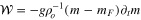 , and the rate of dissipation is
 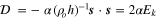 . Other forms of this equation are possible because of the arbitrary reference level in defining potential energy density. A different form of the energy equation that can be derived by combining (6) with other relationships described above is

where  and
and  (other terms defined as above). Alternatively, we may take
 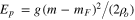 and
and 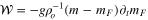 . As we see, the differences in these representations involve the reference level assumed in the definition of the potential energy Ep. Note that while the definition of the rate of work
  depends on the definition of potential energy, the global integral of
  averaged over a tidal cycle is equivalent in all forms and balances the integrated time-averaged
Equations (4)–(5) are solved for the variables  and m using the method described in Tyler (2011). While f and mF are known rather precisely, there is a range of acceptable values for c and α. In this case we calculate solutions from the full range of combinations of these free parameters and draw conclusions from analyses of this collection. That is, we solve the governing equations many times to create the parameter space as a function of the free parameters c and α. Because the parameters c and α may not draw intuitive appeal, we draw reference to derived parameters,
  and
and  The first of these follows from the definition of the shallow-water wave speed given above. The second, Q, can be regarded as the "Q factor" (also called "quality factor," and "specific dissipation") provided that Ek is regarded as the energy density of the system that Q is intended to describe. Specifically, Q is defined as
  multiplied by the energy stored and divided by the energy dissipated per cycle). When the "energy stored" is regarded as Ek and the dissipation is
  (as above), the parameter Q we use can be regarded as the Q factor. More generally, one should regard the
  used here as the non-dimensional timescale associated with the dissipation prescribed by α. For plotting purposes, and to avoid confusion with other uses of Q, we describe the non-dimensional timescale not as Q but rather
  , which is a clear and simple ratio between the forcing and attenuation frequencies. With the Q used above, this is also
  .
.
A.1. Creeping Flow Analytical Solution
A simple analytical solution to the Equations set (4) and (5) is available in the limit of creeping flow, where it is assumed that the acceleration terms on the left side of (4) are negligible compared to the drag term, and the balance must therefore be between the terms on the right side of (4). The momentum equation is then replaced by 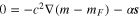 , while the equation for mass conservation (4) remains the same. These two equations can be combined to give

from which the solution for m is easily obtained. Unlike the more generally applicable (4), the reduced form (8) has simple eigenfunctions represented by spherical harmonics which can be used to replace this partial differential equation with an algebraic equation. In this case, the operators translate into coefficients following  ,
, 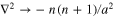 (where a is the radius of the spherical shell and n is the harmonic degree of mF). The solution can be written as the real part of the expression

where the factor  describes the ratio of a speed
  associated with the dissipation (
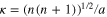 is the associated wavenumber) and the shallow-water wave speed c defined above. (It is insightful to note that
  may be regarded as simply the speed associated with propagation of the tidal forcing.) When the ratio
  is much less than one (i.e., dissipation is small), then the solution is the equilibrium tidal solution
  . When the ratio is much larger than one, we see that the amplitude of the response is generally less than the equilibrium value and the two are ninety degrees out of phase. The solution for the momentum
 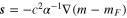 follows directly from the assumed momentum balance described in the first paragraph of this section. Expressions for
  and
and  follow from the solution m,
  as described in the last section. Specifically, one can show that maximum work/dissipation appears when
  . This explains the broad peak in the low Q asymptotic behavior of the complete solutions shown in Figure 4. In the creeping-flow limit, the maximum rate of work/dissipation/heating occurs when the speed at rate which momentum is propagated (c) matches the speed at which momentum is dissipated.
The last sentence may provide the best description of the physical criteria for the peak in dissipation, and it is interesting to compare this with what would be expected in the case of an assumed equilibrium tide. Under the equilibrium-tide assumption, the dilation and contraction of the layer thickness h are prescribed. As a consequence, fluid velocities are required for mass conservation and these velocities increase inversely with h. Dissipation, will increase with flow speed under a power law, which in the simplest case of linear Rayleigh drag involves the rms flow speed squared. A thinner h therefore leads to higher dissipation despite the smaller volume of fluid involved. The physics of this dependence of dissipation on h is quite simple as it only involves two components: conservation of mass, and the expectation that a component of dissipation increases with a power (equal to or higher than 2) of the rms flow speed. One might imagine a circus tent in which the top is pumped up and down at a prescribed rate. The flow speed of air through the sides is set by the conservation of the volume of air and increases inversely with the height of the sides. This process may help to explain how silicate melt within a thin shell may achieve flow speeds large enough to decouple from the more slowly deforming rock matrix through which it moves.
One sees from the results presented that even in the creeping-flow limit the flow speed and therefore the dissipation is not correctly predicted by the equilibrium-tide assumption. The simple flow speeds expected from continuity and the equilibrium assumption show a monotonic dependence on  (and therefore h), while both the creeping-flow analytical solution and the more complete Laplace Tidal Equation solutions at low Q show a non-monotonic dependence of the dissipation on both
  and Q. Of course the failure of the equilibrium-tide assumption in studies of dissipation should not be surprising because the equilibrium tide is formally consistent only with the case of zero dissipation and work.