ADAPTIVE ANNEALED IMPORTANCE SAMPLING FOR MULTIMODAL POSTERIOR EXPLORATION AND MODEL SELECTION WITH APPLICATION TO EXTRASOLAR PLANET DETECTION

The "negligible components" are components that have negligible impact on the proposal function. Their probability masses are much smaller than the others. Based on the principle of survival of the fittest, we delete up to a fixed number of components whose probability masses are smaller than a given threshold T_delete. We then increase the probability masses of the surviving components proportionally with respect to their original values to guarantee that their summation is 1.

This procedure merges overlapped components according to a criterion we term mutual information. The objective is to avoid the coexistence of mixing components that are too overlapped in the proposal, so as to find a more reasonable parsimonious mixture representation of the posterior. To introduce the concept of mutual information, first assume that there are N equally weighted samples $\lbrace \theta ^i\rbrace _{i=1}^N$ drawn from a mixture density function q(·). According to the Monte Carlo principle, q(·) can be approximated by an empirical point-mass function as

$$\begin{equation} q(\theta)\simeq \sum \limits _{n=1}^N\frac{1}{N}\delta (\theta ^i), \end{equation} \tag{ 10 }$$

where δ(θ) denotes the delta-Dirac mass function located at θ. Denoting (m|θⁿ) the posterior mass in the event that θⁿ belongs to component m, we have

$$\begin{equation} \epsilon (m|\theta ^n)=\frac{\alpha _m f_m(\theta ^n|\xi _m)}{q(\theta ^n|\psi)}. \end{equation} \tag{ 11 }$$

It is intuitive that the components j, k contain completely overlapped information, if the identity (j|θⁿ) = (k|θⁿ) is satisfied for n = 1, 2, ..., N. Based on this heuristic, the mutual information between components j, k is defined as

$$\begin{equation} {{\mathsf MI}}(j,k)=\frac{(Z_j-\bar{Z}_j)^T(Z_k-\bar{Z}_k)}{\Vert Z_j-\bar{Z}_j\Vert \cdot \Vert Z_k-\bar{Z}_k\Vert }, \end{equation} \tag{ 12 }$$

where Z_m = ((m|θ¹), ..., (m|θ^N))^T, the superscript T denotes the transposition operation, || · || the Euclidean norm, and $\bar{Z}_m= {1}/{N}\sum _{n=1}^N \epsilon (m|\theta ^n){\bf 1}_N$. Here, 1_n denotes the n-dimensional column vector with all elements being 1.

Note that ${{\mathsf MI}}(j,k)\in [-1,1], j,k\in \lbrace 1,\ldots,M\rbrace ^2$, and ${{\mathsf MI}}(j,k)=1$ iff the jth and kth components are identical. Within the IS framework, each data point θⁿ is associated with an importance weight, wⁿ. Correspondingly $\bar{Z}_m$ becomes $\sum _{n=1}^N w^n \epsilon (m|\theta ^n)$, and the mutual information between j, k turns to be

$$\begin{equation} {{{\mathsf MI}}(j,k)=\frac{(Z_j\,{-}\,\bar{Z}_j)^T \mbox{diag}(w^1,\ldots,w^N)(Z_k\,{-}\,\bar{Z}_k)}{\sqrt{\sum _{n=1}^N w^n(\epsilon (j|\theta ^n)\,{-}\,\bar{Z}_j)^2}\sqrt{\sum _{i=1}^N w^n(\epsilon (k|\theta ^n)\,{-}\,\bar{Z}_k)^2}}}, \end{equation} \tag{ 13 }$$

where diag(·) denotes the diagonal matrix with elements in the parentheses.

For each pair of two components j, k, if ${{\mathsf MI}}(j,k)$ is bigger than a given threshold T_merge, we merge them into one using the following operations:

$$\begin{eqnarray} \ \ \alpha _{r}&=&\alpha _{j}+\alpha _{k} \end{eqnarray} \tag{ 14 }$$

$$\begin{eqnarray} \qquad \xi _{j}&=&\frac{\alpha _{j}\xi _{j}+\alpha _{k}\xi _{k}}{\alpha _{r}} \end{eqnarray} \tag{ 15 }$$

$$\begin{eqnarray} \alpha _{j}&=&\alpha _{r},\ \ \ \ \ \end{eqnarray} \tag{ 16 }$$

and then we subtract one for M.

This procedure is developed for exploring the posterior, especially the parameter subspace that is indeed important for the posterior but has been neglected in q so far. We add new components centered at the samples of the highest importance weights, and tune their parameters for exploring local structures of the posterior.

We denote the highest weight sample using θ^s, s ∈ {1, 2, ⋅⋅⋅, N}. First, we compute the ESS based on current IS draws, and compare it with a given threshold ESS_thr. If the current ESS is smaller than ESS_thr, we perform the add operation as follows.

• 1.  
  Design a trial density function f_trial(·) to approximate the local structure of the target function around θ^s.
• 2.  
  Build up a trial mixture proposal q_trial by combining f_trial(·) with q as q_trial = α_trialf_trial  +  (1  −  α_trial)q, where 0 < α_trial < 1 denotes the initial probability mass specified to f_trial. Denote the parameter of q_trial by ψ_trial.
• 3.  
  Use q_trial as the proposal function and perform IS. Then, we select out the particle with the highest importance weight and label it $\theta _{{\rm trial}}^{s}$. We then update ESS based on current IS draws. If the new ESS value is bigger than the older one, it means that the add operation is useful for increasing the ESS value, so we update ψ = ψ_trial and $\theta ^{s}=\theta _{{\rm trial}}^{s}$ and go to step 1; otherwise, go to the next step.
• 4.  
  Update ψ via an iteration of the EM operation, which is presented in Section 3.4.
• 5.  
  Perform IS again and update the location of θ^s.
• 6.  
  Calculate ESS. If the current ESS is bigger than a given threshold ESS_thr, end this procedure; otherwise, go to Step 1.

A crucial issue of the above operation is how to explore the local region around the highest weight sample. It is clear intuitively that we must get some samples from the interesting region for exploration. We do this in Step 1 via a routine IS procedure that provides a Monte Carlo estimate of that local region. The parameter of f_trial is then updated to let f_trial resemble the local shape of the target function.

In the mixture defined by Equation (6), we select the mixture components to be Student's t-distributions, whose heavy-tail property is desirable for constructing IS proposal densities. When a d dimensional random variable Y follows the multivariate Student's t-distribution $\mathcal {S}(\cdot |\mu,\Sigma,v)$ with center μ, positive definite inner product matrix Σ, and degrees of freedom v ∈ (0, ∞], the density function of Y is shown to be

$$\begin{equation} \mathcal {S}(Y|\mu,\Sigma,v)=\frac{\Gamma (\frac{v+d}{2})|\Sigma |^{-0.5}}{(\pi v)^{0.5d}\Gamma (\frac{v}{2})\lbrace 1+\delta (Y,\mu,\Sigma)/v\rbrace ^{0.5(v+d)}}, \end{equation} \tag{ 17 }$$

where

$$\begin{equation} \delta (Y,\mu,\Sigma)=(Y-\mu)^T \Sigma ^{-1}(Y-\mu) \end{equation} \tag{ 18 }$$

denotes the Mahalanobis squared distance from Y to μ with respect to Σ. Substituting f_m(θ|η) with $\mathcal {S}(\theta |\mu _m,\Sigma _m,v)$ in Equation (6), we get the Student's t-mixture model:

$$\begin{equation} q(\theta |\psi)=\sum \limits _{m=1}^M \alpha _m \mathcal {S}(\theta |\mu _m,\Sigma _m,v), \sum \limits _{m=1}^M \alpha _m=1, \alpha _m\ge 0, \end{equation} \tag{ 19 }$$

for which the adjustable parameters include M, μ_m, Σ_m, α_m, m = 1, 2, ..., M. Based on a weighted sample set $\lbrace \theta ^n,w^n\rbrace _{n=1}^N$, the E and M steps update values of α_m, μ_m, and Σ_m in q as (Cappé et al. 2008)

E step:

$$\begin{equation} {\alpha _m}^{\prime }=\sum \limits _{n=1}^N f_m(\theta ^n|\mu _m,\Sigma _m)\epsilon (m|\theta ^n), \end{equation} \tag{ 20 }$$

M step:

$$\begin{eqnarray} {\mu _m}^{\prime }&=&\frac{\sum \limits _{n=1}^N w^n \epsilon (m|\theta ^n)u_m(\theta ^n)\theta ^n }{\sum \limits _{n=1}^N w^n \epsilon (m|\theta ^n)u_m(\theta ^n)}, \end{eqnarray} \tag{ 21 }$$

$$\begin{eqnarray} {\Sigma _m}^{\prime }&=&\frac{\sum \limits _{n=1}^N w^n \epsilon (m|\theta ^n)u_m(\theta ^n)C_n }{\sum \limits _{n=1}^N w^n \epsilon (m|\theta ^n)}, \end{eqnarray} \tag{ 22 }$$

where

$$\begin{equation} u_m(\theta)=\frac{v+d}{v+(\theta -\mu _m)^T(\Sigma _m)^{-1}(\theta -\mu _m)} \end{equation} \tag{ 23 }$$

and C_n = (θⁿ − μ_m)(θⁿ − μ_m)^T, is calculated by Equation (11), d is the dimension of θ, and A' is an updated value of A. More details about the EM operation can be found, for example, in Mclachlan & Krishnan (1997) and Mclachlan & Peel (2000).

Here, several guidelines for initialization and specification of the involved tuning parameters of the algorithm are provided.

The AAIS algorithm is started by initializing the proposal q(· |ψ₀), which is in the form of a Student's t-mixture, defined by Equation (19). It is practical to select q(· |ψ₀) to be a dispersive distribution over the parameter space, if there is no prior knowledge about the posterior before running the algorithm. We argue that the efficiency of the algorithm is not dependent on the initial value of ψ₀, as discussed in Section 3.7. This argument has also been corroborated by several simulation studies. For example, in the Rastrigin case in Section 3.8.1, a single-mode initialization with only one component results in a final proposal that approximates a highly multimodal posterior.

In every iteration, say the ith one, the annealing temperature λ_i needs to be specified. Here, we present an adaptive approach to determine λ_i online. First, note that the annealed target density p_i(θ) is a function of λ, as shown in Equation (7). p_i(θ) then determines the importance weights of the importance samples drawn from proposal q(· |ψ_{i − 1}). Since there is a certain relationship between the ESS and the importance weights through Equation (4), the ESS can be treated as a function of λ. We denote the function as

$$\begin{equation} \mbox{ESS}_i\triangleq g(\lambda), \end{equation} \tag{ 24 }$$

where the subscript identifies the iteration index. Based on λ_{i − 1}, λ_i is specified by

$$\begin{equation} \lambda _{i}=\underset{\lambda \in (\lambda _{i-1},1]}{\arg \min }\Vert g(\lambda)-\beta \cdot \mbox{ESS}_{i-1}\Vert ^2, \end{equation} \tag{ 25 }$$

where ESS_{i − 1} is calculated based on importance weights that are associated with p_{i − 1}(θ), and β ∈ (0, 1) is a parameter controlling the extent to which p_i(·) differs from p_{i − 1}(·). Empirically, we select β = 0.8 to guarantee a smooth transition from p_{i − 1}(·) to p_i(·).

The annealing temperature ladder can also be specified empirically in an offline manner. The linear incremental ladder, e.g., [0.1, 0.2, ..., 0.9, 1], the exponential incremental ladder, e.g., [0.0001, 0.001, 0.01, 0.1, 1], and the hybrid ladder, e.g., [0.0001, 0.001, 0.01, 0.1, 0.4, 0.7, 1] are all candidate choices for practical use. The efficiency of each choice can be monitored by the accompanying ESS outputs of every iteration of the algorithm. In our experimental studies, we just adopt the offline methods for saving computing resources.

T_delete is the single tuning parameter in the delete operation, and its value is set online. The guideline is to guarantee that T_delete ≪ 1/M. For example, if there is now 10⁴ mixing components in the proposal, it is then reasonable to set T_delete = 10⁻⁶, but if there are only three components, then a value 1/100 is effective enough for use.

In the merge operation, the tuning parameter T_merge should be specified beforehand. T_merge denotes a quantization for the greatest overlapping level allowed among the mixing components. An empirical choice for T_merge is 0.85.

In the add operation, the trial component f_trial is in the form of Student's t, as shown in Equation (17). The only parameter that needs to be artificially specified is Σ_trial. A typical choice is just to specify Σ_trial to be a unit diagonal matrix for simplicity, unless there is any available prior knowledge on the local structure around the highest weight IS draw. The probability mass of the new added component, i.e., α_trial, is initially set as the averaged probability mass of the mixing components.

In setting ESS_thr and the particle size N, we mainly consider the dimensions and complexity of the problem. For less than three-dimensional (3D) cases, we empirically set ESS_thr = 0.9N with N = 4 × 10³; for four- to seven-dimensional cases, an empirical choice is ESS_thr = 0.4N with N = 10⁴; for eight- to twelve-dimensional cases, ESS_thr = 0.3N with N = 2 × 10⁵ is usually set. The highest dimensional case for which the algorithm has been evaluated is the computation of the marginal likelihood of a three-planet model whose parameter is 17 dimensions. For that case, we set ESS_thr = 0.2N and N = 10⁶.

Regarding the delete/merge/add operations described above, one may wonder what the effects of each one are on the other two. For example, is it possible that the new added component just happens to meet the condition of merging or deleting, or can these three operations be interchangeable? We argue that the add operation is independent of the other two. According to our algorithm design, the new added component is always located around the highest weight sample, whose location is separated from the well-supported area of the parameter space. Basically, the new added component is unlikely to meet the condition of merging. The initialized probability mass of the newly added component can be strictly controlled to guarantee that the new component cannot be deleted upon its generation. In summary, the add operation can be performed prior to or after any one of the other two. However, the delete operation should be performed prior to the other two. This can prevent the algorithm from spending unnecessary computing resources on the negligible components. Since only a limited number of negligible components are allowed to be deleted in one iteration, the new proposal q(·) are guaranteed to be effective.

The proposed AAIS algorithm has connections to existing adaptive IS (AIS) methods, e.g., Evans (1991), Oh & Berger (1993), Cappé et al. (2008, 2004), and West (1993), to name just a few. Such AIS methods are featured in an iterative manner in which the proposal function is updated.

Recently, a state-of-the-art AIS algorithm called PMC has been used in the area of astrophysics (Kilbinger et al. 2010; Wraith et al. 2009). PMC was first proposed in statistical literature (Cappé et al. 2004, 2008). The appeal of PMC lies in the usage of a flexible mixture type proposal and a simple EM-based mechanism to tune the mixture parameter, which makes it an efficient approach to handle some multimodal posteriors. The shortcomings of PMC accompany its merit. First, in the PMC algorithm, the number of mixing components is restricted to be a pre-determined constant, which is clearly a strong limitation. Furthermore, PMC totally relies on an EM mechanism to update the parameter values of the mixture proposal, while EM itself is a local optimization/searching technique whose efficiency largely depends on the initialization. Thus, the efficiency of the algorithm is highly dependent on the initial choice of the proposal, which has already been pointed out by Kilbinger et al. (2010).

The proposed AAIS algorithm distinguishes itself from existing AIS methods (including PMC) in the following aspects.

First, instead of approximating the posterior p(·) directly, as in AIS, the new algorithm seeks to tailor a prescribed proposal to approximate a series of annealed distributions (p_i(·) in Equation (7)) one by one.

Second, in the AAIS algorithm a set of newly developed operations termed delete, merge, and add is proposed to work in tandem with the EM procedure to tailor the number of mixing components online.

The combination of the embedded annealing strategy and the developed delete/merge/add operations creates a real difference between the proposed AAIS algorithm and the other existing AIS methods. The annealed distributions provide a smooth intermediate transition from the initial proposal to the posterior, while there is a good chance that the initial proposal differs greatly from the posterior in shape. The delete/merge/add processes fill gaps in the EM method by providing a way to tailor the number of mixture components online, by virtue of which the limitation stemming from the local property of the EM is broken. With the aid of the delete/merge/add operations, the annealing strategy truly comes into play, giving AAIS the desired global searching property and making the efficiency of the algorithm not dependent on the initialization.

For complicated posteriors, e.g., the Rastrigin function as introduced in Section 3.8.1, which has massive peaky modes, it is shown that PMC is not able to discover the overall structure of the posterior, even if the mixing component number is preset to be a large value. We argue that the above phenomenon stems from the inherent local searching property of PMC.

In this section, we perform simulation studies to test the capability of the developed AAIS method in exploring and approximating complex posteriors.

3.8.1. Example 1: Rastrigin Function

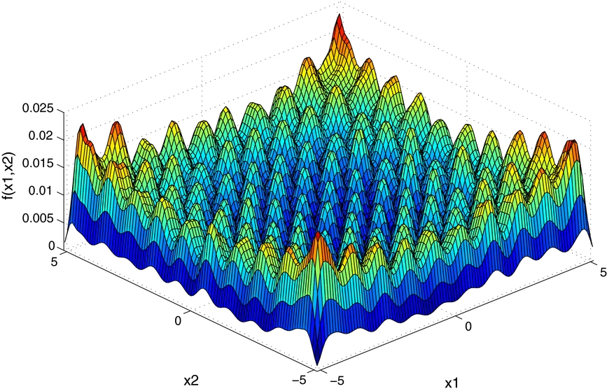
The Rastrigin function is a typical example of a nonlinear and highly multimodal function, which is widely used as a performance test problem for optimization algorithms, e.g., in Mühlenbein et al. (1991). The Rastrigin function is defined by

$$\begin{equation} f(x)=10d+\sum _{i=1}^d[x_i^2-10\cos (2\pi x_i)], \end{equation} \tag{ 26 }$$

where d denotes dimensions. The global minimum f(x*) = 0 at x* = (0, ⋅⋅⋅, 0). As usual, the function is evaluated on the hypercube x_i ∈ [ − 5.12, 5.12] for all i = 1, ⋅⋅⋅, d. It is shown in Figure 1 in its two-dimensional (2D) form.

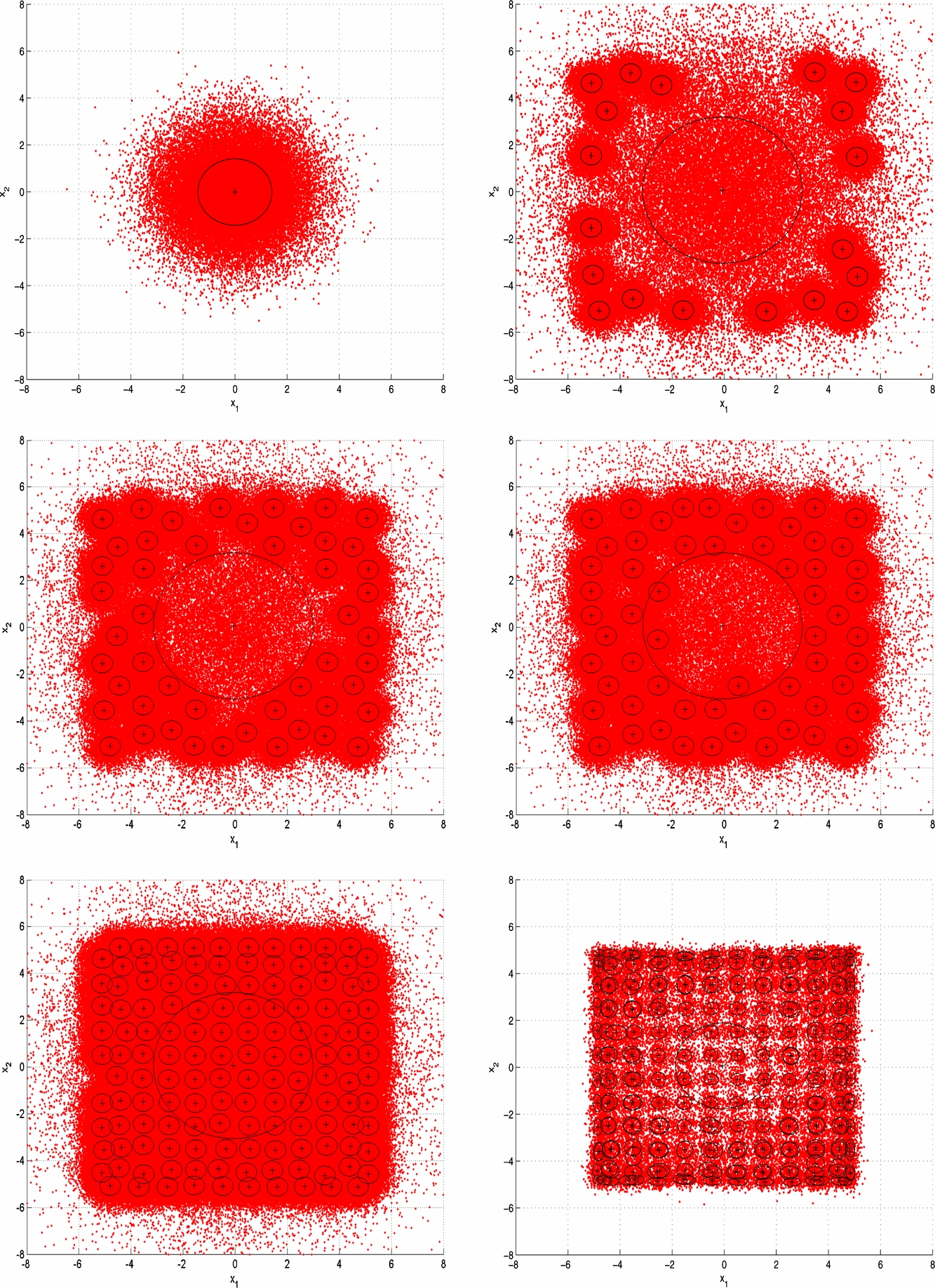
Zoom In Zoom Out Reset image size

Here, we set the target function to be proportional to the 2D Rastrigin function, i.e., p(θ)∝f(x), θ≜x. The purpose is to test the capability of our AAIS algorithm in dealing with highly multimodal target distributions. The mixture proposal final output of an example run of the AAIS is shown in Figure 2. In this example run, the AAIS algorithm is initialized with only one component; its intermediate sampling and proposal output are shown in Figure 3. As can be seen, the AAIS algorithm adaptively tunes the number of surviving components and finally gives an accurate estimate of the shape of the posterior.

Zoom In Zoom Out Reset image size

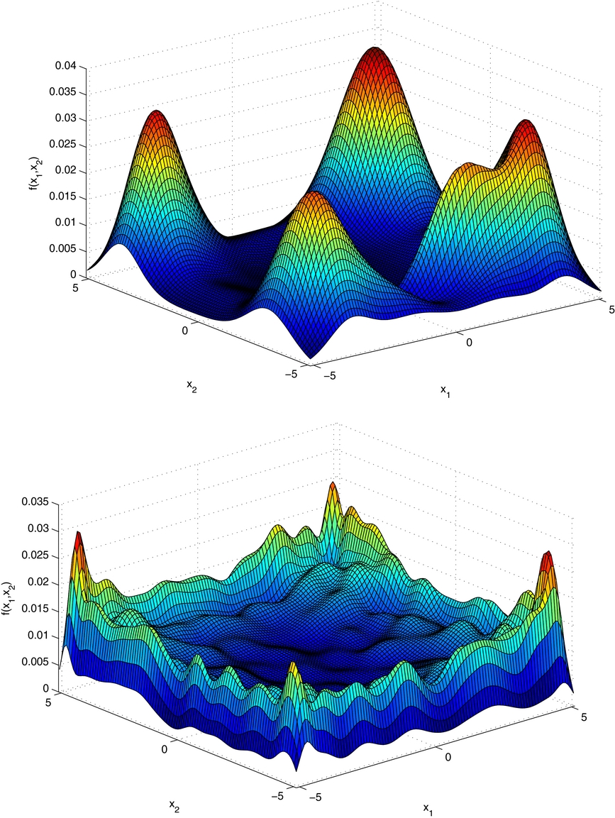
Zoom In Zoom Out Reset image size

In order to compare the performance of the AAIS with that of PMC, the mixture proposal function output by a typical run of PMC is presented in Figure 4. It is shown that the result is highly dependent on the initialization and that the PMC algorithm is incapable of discovering the overall structure of the posterior, which corroborates arguments made in Section 3.7.

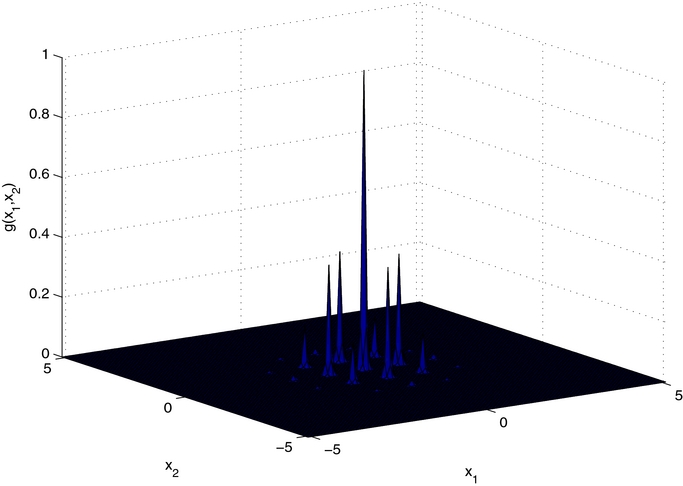
Zoom In Zoom Out Reset image size

Now we consider the application of AAIS for finding the global minimum of the ten-dimensional Rastrigin function. As the algorithm always tends to sample/explore areas with higher density values, it is natural to adapt it to search maxima rather than minima. So we transform the Rastrigin function to g(x) = exp (− f(x)), and then the task becomes looking for the global maxima. The transformed function is shown in Figure 5 in its 2D form. We evaluate the function values corresponding to all those samples generated during the running process of the algorithm and then output the one with the biggest function value as the final solution. The AAIS algorithm is equipped with a temperature ladder [0.0001, 0.001, 0.01, 0.1, 0.2, 0.4, 0.8, 1] and a particle size N = 10⁵. The truly global maximum 1 is only reached at x* = (0, ⋅⋅⋅, 0), but the algorithm could find a solution better than 0.99 in 8 out of 10 runs, with an overall best solution being 0.9976 with corresponding x = [0.0004, −0.0014, −0.0014, −0.0016, 0.0005, 0.0001, 0.0007, −0.0010, −0.0004, −0.0018]. In the other two runs, the AAIS algorithm always found one of the local minima.

Zoom In Zoom Out Reset image size

3.8.2. Example 2: Three-dimensional Flared Helix

Here, the posterior is simulated to be proportional to a cylindrical function with a standard Gaussian cross-section (in (x, y)) that has been deformed (in z) into a helix with varying diameters. The helix performs three complete turns. The shape of this function is illustrated in Figure 6. The function is normalized to integrate to exactly 60. We wonder if the shape of the output mixture proposal from AAIS can match that of the posterior.

Zoom In Zoom Out Reset image size

For AAIS, we initialize the proposal q with 10 equally weighted mixing Student's t components, whose centers are uniformly distributed over the parameter space. Ten iterations of the algorithm are performed with a linear incremental ladder [0.1, 0.2, ..., 0.9, 1]. The PMC algorithm (Cappé et al. 2008) is also included for performance comparison. We initialize PMC the same as for AAIS, and also run it with 10 iterations to output the final proposal function.

In Figure 7 we plot 2000 random samples drawn from the mixture proposals outputted by AAIS and PMC, respectively. It is shown that AAIS successfully explored those three complete turns, while PMC missed the last half turn in the helix function.

Zoom In Zoom Out Reset image size

We then test if the proposed AAIS can give a good estimation of the integral of the test function. The benchmark PMC algorithm is also included for comparison. We show the results in Table 1. It is shown that AAIS performs much better than PMC, as it gives a much more accurate estimate to the real answer.

Table 1. 3D Flared Helix Example

	ESS/N	Estimate of the Integral (Real Answer is 60)
AAIS	0.4459	59.7 ± 2.0
PMC	0.1525	47.2 ± 3.3

Note. Quantitative performance comparison.

Download table as:  ASCIITypeset image

3.8.3. Example 3: Outer Product of Seven Univariate Densities

Here, our concern is whether good results gained from the above 2D and 3D examples imply good results in a high-dimensional target function with two or more target modes. To test this concern, we use as a target function the outer product of seven univariate distributions normalized to integrate to exactly 1. These seven distributions are as follows:

• 1.  
  $\displaystyle\frac{3}{5}\mathcal {G}(10+x|2,3)+ \displaystyle\frac{2}{5}\mathcal {G}(10-x|2,5)$
• 2.  
  $\displaystyle\frac{3}{4}sk\mathcal {N}(x|3,1,5)+\displaystyle\frac{1}{4}sk\mathcal {N}(x|-3,3,-6)$
• 3.  
  $\mathcal {S}(x|0,9,4)$
• 4.  
  $\displaystyle\frac{1}{2}\mathcal {B}(x+3|3,3)+\displaystyle\frac{1}{2}\mathcal {N}(x|0,1)$
• 5.  
  $\displaystyle\frac{1}{2}\varepsilon (x|1)+\displaystyle\frac{1}{2}\varepsilon (-x|1)$
• 6.  
  $sk\mathcal {N}(x|0,8,-3)$
• 7.  
  $\displaystyle\frac{1}{8}\mathcal {N}(x|-10,0.1)+\displaystyle\frac{1}{4}\mathcal {N}(x|0,0.15)+\displaystyle\frac{5}{8}\mathcal {N}(x|7,0.2)$.

Here, $\mathcal {G}(\cdot |\alpha,\beta)$ denotes the gamma distribution, $\mathcal {N}(\cdot |\mu,\sigma)$ the normal distribution, $sk\mathcal {N}(\cdot |\mu,\sigma,\alpha)$ the skew-normal distribution, $\mathcal {S}(\cdot |\mu,s,df)$ the Student's t-distribution, $\mathcal {B}(\cdot |\alpha,\beta)$ denotes the beta distribution, and ε(· |λ) the exponential distribution. Dimension 2 has two modes bracketing a deep ravine, dimension 4 has one low, broad mode that overlaps a second sharper mode, and dimension 7 has three distinct, well-separated modes. Only dimension 5 is symmetric. There is a range of tail behavior as well, from Gaussian to heavy-tailed.

We initialize for AAIS 50 equally weighted mixing components. The centers of these components for each dimension are uniformly distributed over [ − 10, 10]. A linear incremental ladder [0.1, 0.2, ..., 0.9, 1] is used. We include PMC here for performance comparison, which is initialized identically, and run with 10 iterations.

In Figure 8 we depict the scatter plot of random samples drawn from the resulting mixture proposals outputted by AAIS and PMC, respectively. It is shown that the proposed AAIS algorithm manages to find all the modes in the target function, while PMC fails to detect the target modes in the second and seventh dimension.

Zoom In Zoom Out Reset image size

For this case, AAIS also gives an accurate estimate to the integral of the target function, as shown in Table 2.

Table 2. Seven-dimensional Outer Product Example

	ESS/N	Estimate of the Integral (Real Answer is 1)
AAIS	0.4948	1.0011 ± 0.0303
PMC	0.2454	0.4675 ± 0.0246

Note. Quantitative performance comparison.

Download table as:  ASCIITypeset image

If a star does not host any orbiting planets, then the RV measurements will be roughly constant over any period of time, varying due to the "stellar jitter," the random fluctuations in a star's luminosity, or fluctuations stemming from other systematic sources, e.g., starspots. In the zero-planet model, the ith element of the RV data, v_i, is Gaussian-distributed as

$$\begin{equation} v_i \mid {\cal {M}}_0\sim \mathcal {N}\left(C,\sigma _i^2+s^2\right), \end{equation} \tag{ 27 }$$

with mean C and variance $\sigma ^2_i \,{+}\, s^2$. C denotes the constant center-of-mass velocity of the star relative to earth, s the square root of the "stellar jitter," and the additional variance component $\sigma ^2_i$ is a calculated error of v_i due to the observation procedure.

In ${\cal {M}}_1$,

$$\begin{equation} v_i \mid {\cal {M}}_1 \sim \mathcal {N}\left(C +\bigtriangleup V(t_i|\phi),\sigma _i^2+s^2\right), \end{equation} \tag{ 28 }$$

where ▵V(t_i|ϕ) is the velocity shift caused by presence of the planet. Such a velocity shift is a family of curves parameterized by a five-dimensional vector ϕ≜(K, P, e, ω, μ₀) as follows:

$$\begin{equation} \bigtriangleup V(t|\phi)=K[\cos (\omega +T(t))+e\cos (\omega)], \end{equation} \tag{ 29 }$$

where T(t) is the "true anomaly at time t" given by

$$\begin{equation} T(t)=2\arctan \left[\tan \left(\frac{E(t)}{2}\right)\sqrt{\frac{1+e}{1-e}}\right], \end{equation} \tag{ 30 }$$

and E(t) is called the "eccentric anomaly at time t," which is the solution to the transcendental equation

$$\begin{equation} E(t)-e\sin (E(t))=\mbox{mod}\left(\frac{2\pi }{P}t+\mu _0,2\pi \right). \end{equation} \tag{ 31 }$$

In the above expressions, K denotes the velocity semi-amplitude, P the orbital period, e the eccentricity (0 ⩽ e ⩽ 1), ω the argument of periastron (0 ⩽ ω ⩽ 2π), and μ₀ the mean anomaly at time t = 0, (0 ⩽ μ ⩽ 2π). The parameters C, K, and s have the same unit as velocity, the velocity semi-amplitude K is usually restricted to be non-negative to avoid identification problems, and C may be positive or negative. The eccentricity parameter e is unitless, with e = 0 corresponding to a circular orbit, and a larger e means more eccentric orbits. Periastron is the point at which the planet is closest to the star and the argument of periastron ω measures the angle at which we observe the elliptical orbit. The mean anomaly μ is the angular distance of a planet from periastron.

If there are p ⩾ 1 planets, the expected velocity is C + ▵V(t_i|ϕ₁, ..., ϕ_p). The overall velocity shift ▵V is the summation of velocity shifts of each individual planet, i.e.,

$$\begin{equation} \bigtriangleup V(t_i|\phi _1,\ldots,\phi _p)=\sum _{j=1}^p \bigtriangleup V(t_i|\phi _j). \end{equation} \tag{ 32 }$$

Given competing models ${\cal {M}}_0$, ${\cal {M}}_1$, ..., ${\cal {M}}_M$, we do Bayesian model selection to determine the number of planets. Bayesian model selection requires calculation of marginal likelihoods. Taking ${\cal {M}}_p$, for example, its marginal likelihood is calculated as

$$\begin{equation} l({\cal {M}}_p)=\int _{\Theta _p} p(\mathbf {v}\mid \theta _p,{\cal {M}}_p)p(\theta _p\mid {\cal {M}}_p)d\theta _p, \end{equation} \tag{ 33 }$$

where v≜(v₁, ...v_n), n is the sample size of the RV observations, θ_p the parameter of ${\cal {M}}_p$, Θ_p the value space of θ_p, $p(\theta _p \mid {\cal {M}}_p)$ the prior, and $p(\mathbf {v}\mid \theta _p,{\cal {M}}_p)$ the likelihood. It is worth noting that, without forced identifiability (i.e., not imposing any order on the planetary parameters) there are at least p! modes in the likelihood; therefore, the likelihood value should be divided by p!. Bayes Factors for comparing the p planet model to the 0 planet model can be expressed as

$$\begin{equation} {{\mathsf BF}}({\cal {M}}_p:{\cal {M}}_0)=\frac{l({\cal {M}}_p)}{l({\cal {M}}_0)}. \end{equation} \tag{ 34 }$$

The posterior of the p planet model is calculated with

$$\begin{equation} p({\cal {M}}_p \mid \mathbf {v}) = \frac{{{\mathsf BF}}({\cal {M}}_p:{\cal {M}}_o) O({\cal {M}}_p: {\cal {M}}_0)}{\sum _{ j= 1}^{M} {{\mathsf BF}}({\cal {M}}_j:{\cal {M}}_o) O({\cal {M}}_j: {\cal {M}}_0)}, \end{equation} \tag{ 35 }$$

where $O({\cal {M}}_p: {\cal {M}}_0)$ is the prior odds of having p planets to 0 planet. We present the related priors in the following subsection.

We adopt priors recommended in (Ford & Gregory 2006; Bullard 2009) due to their approximate realism and mathematical tractability. For all models under investigation, the prior of C is uniformly distributed over an interval [C_min, C_max] defined by a lower limit C_min and upper limit C_max of C, with C_max > C_min, i.e.,

$$\begin{eqnarray} p_C(C) &=& \left\lbrace \begin{array}{@{}cl} \frac{1}{C_{\max }\,{-}\,C_{\min }} & \quad \mbox{for }\; C_{\min }\le C\le C_{\max },\\ 0& \quad \mbox{otherwise}. \\ \end{array} \right. \end{eqnarray} \tag{ 36a }$$

log (s_min + s) is uniformly distributed over the interval [log (s_min), log (s_max)]:

$$\begin{eqnarray} p_{s}(s) & =& \left\lbrace \begin{array}{@{}cl} \frac{1}{ \log \left(1\,{+}\,\frac{s_{\max }}{s_{\min }}\right)} \cdot \frac{1}{s_{\min }\,{+}\,s} & \quad \mbox{for } 0 < s \le s_{\max } \\ 0 & \quad \mbox{otherwise.} \\ \end{array} \right. \end{eqnarray} \tag{ 36b }$$

The joint prior on (C, s²) can be viewed as a modified independent Jeffrey's prior as C_min → −∞, C_max → ∞, s_min → 0, s_max → ∞, which leads to well-defined posterior distributions and Bayes Factors even in the limit.

For a p > 0 planet model, without other prior information, each pair of ϕ_i and ϕ_j (i ≠ j, i, j ∈ [1, p]) have identical independent priors. As in (Ford & Gregory 2006; Bullard 2009), we specify an independent prior for elements of each ϕ_j, j = 1, 2, ..., p in a transformed parameter space:

$$\begin{eqnarray} x &=& e\cos \omega \quad y= e\sin \omega \quad z = (\omega +\mu _0)\; {\rm mod}\; {2}\pi\nonumber \\ \dot{P} &=& \log P \quad \dot{K} =\log K\nonumber \end{eqnarray}$$

leading to $\dot{\phi }_j \equiv (\dot{K}_j, \dot{P}_j, x_j, y_j, z_j)$. The Poincaré variables x and y greatly reduce the very strong correlations between μ₀ and ω, which is particularly important for low eccentricity orbits, where the parameters are nearly unidentifiable. The use of z further reduces correlations between the parameters ω and μ₀ when e ≪ 1, but has little effect for large e. Bullard (2009) recommended using the log transformation of P and K because the posteriors are more Gaussian in these coordinates, which led to improved posterior simulation. In the transformed parameter space, the prior distribution for ϕ is

$$\begin{equation} p_{\dot{\phi }}(\dot{\phi })=c_\phi \cdot \exp \dot{K}\cdot \frac{1}{1+\frac{\exp \dot{K}}{K_{\min }}}\cdot \frac{1}{\sqrt{x^2+y^2}} \end{equation} \tag{ 37a }$$

for $\log (K_{\min }) < \dot{K} \le \log (K_{\max })$, $\log (P_{\min })\le \dot{P}\le \log (P_{\max })$, x² + y² < 1, and 0 ⩽ z ⩽ 2π, where the normalizing constant is

$$\begin{equation} c_\phi =\frac{1}{\log \left(1+\frac{K_{{\rm max}}}{K_{\min }}\right)}\cdot \frac{1}{K_{\min }}\cdot \frac{1}{\log \left(\frac{P_{\max }}{P_{\min }}\right)}\cdot \left(\frac{1}{2\pi }\right)^2. \end{equation} \tag{ 37b }$$

We list the constants used in the specification of the prior in Table 3, which are set based on physical realities (e.g., an orbit with too small a period will result in the planet getting consumed by the star).

We simulate 10 RV observations from a star hosting one planet with P = 100 days, K = 20 ms⁻¹, e = 0.5, μ₀ = 1, C = 0, and s = 1.5. The corresponding periodogram is shown in Figure 9. Then, we run the AAIS algorithm to estimate parameters of the single-planet model ${\cal {M}}_1$ and predict the RV curve during the observation period. In Figure 10, the predicted RV curve along with the corresponding credible interval is compared with the true RV curve. As is shown, the true RV answer falls within the ±1 standard error (68%) credible interval of the prediction almost everywhere, which confirms the accuracy of the parameter estimation. The marginal likelihoods of ${\cal {M}}_0$, ${\cal {M}}_1$, and ${\cal {M}}_2$ are estimated by AAIS to be 4.74  ×  10⁻⁴⁵, 3.14  ×  10⁻¹⁶, and 4.95  ×  10⁻¹⁷, respectively. So the corresponding Bayes factors are ${{\mathsf BF}}\lbrace \mathcal {M}_1:\mathcal {M}_0\rbrace =6.62\times 10^{28}$, ${{\mathsf BF}}\lbrace \mathcal {M}_1:\mathcal {M}_2\rbrace =6.33$, which supports the existence of a single planet.

Zoom In Zoom Out Reset image size

Zoom In Zoom Out Reset image size

Tinney et al. released this data set and claimed to support an orbit of 190.5 ± 3.0 days (Tinney et al. 2003). Gregory then did a Bayesian re-analysis on this data set and reported three possible orbits, with periods $127.88_{-0.09}^{+0.37}$, $190.4_{-2.1}^{+1.8}$, and $376.2_{-4.3}^{+1.4}$ days, respectively (Gregory 2005). Gregory also discussed the possibility of an additional planet and reported that the Bayes factor is less than 1 when comparing $\mathcal {M}_2$ with $\mathcal {M}_1$ (Gregory 2005).

We use the proposed AAIS algorithm to estimate the marginal likelihoods of $\mathcal {M}_0$, $\mathcal {M}_1$, and $\mathcal {M}_2$, respectively. The result is summarized in Table 4. These estimates are reliable, which is indicated by the performance metric ESS/N, which is also included in Table 4. The resulting Bayes Factors are shown in Table 5, which supports $\mathcal {M}_1$ the most. This result is consistent with conclusions made in Tinney et al. (2003) and Gregory (2005).

Table 4. HD 73526 Tinney et al. (2003) Data Case: Estimated Marginal Likelihoods.

	Marginal Likelihood	ESS/N
$\mathcal {M}_0$	5.9013 × 10−50 ± 5.1325 × 10−52	0.9320
$\mathcal {M}_1$	4.4886 × 10−41 ± 3.2093 × 10−42	0.5698
$\mathcal {M}_2$	1.5511 × 10−42 ± 3.2878 × 10−43	0.3458

Download table as:  ASCIITypeset image

Table 5. HD 73526 (Tinney et al. 2003) Data Case: Estimated Bayes Factors

BF$\lbrace \mathcal {M}_1:\mathcal {M}_0\rbrace$	BF$\lbrace \mathcal {M}_2:\mathcal {M}_1\rbrace$
7.606 × 108	0.03456

Download table as:  ASCIITypeset image

Focusing on $\mathcal {M}_1$, we investigate the posterior by drawing random samples from its approximation proposal given by AAIS. We show a scatter plot of the samples in Figure 11. It is clear that there are two modes in the period P, which are $P_1=190.1_{-1.5}^{+2.2}$ and $P_2=375.5_{-2.5}^{+2.0}$, respectively.

Zoom In Zoom Out Reset image size

Tinney et al. released another data set on the star HD 73526 (Tinney et al. 2006), which contains more RV data components than in Tinney et al. (2003). Such a data set was claimed to have two planets (Tinney et al. 2006).

We estimate the marginal likelihoods of $\mathcal {M}_0$, $\mathcal {M}_1$, $\mathcal {M}_2$, and $\mathcal {M}_3$, respectively, via the proposed AAIS algorithm. The result is shown in Table 6. The estimates are reliable, as indicated by the metric ESS/N. The resulting Bayes Factors are listed in Table 7, and indicate that it most likely has two planets.

Table 6. HD 73526 (Tinney et al. 2006) Data Case: Calculated Marginal Likelihoods

	Marginal Likelihood	ESS/N
$\mathcal {M}_0$	8.9566 × 10−77 ± 1.0852 × 10−78	0.9510
$\mathcal {M}_1$	5.8519 × 10−70 ± 1.7077 × 10−71	0.6545
$\mathcal {M}_2$	4.8122 × 10−65 ± 1.4284 × 10−66	0.2034
$\mathcal {M}_3$	1.7981 × 10−72 ± 2.6248 × 10−73	0.1281

Download table as:  ASCIITypeset image

Table 7. HD 73526 (Tinney et al. 2006) Data Case: Calculated Bayes Factors

BF$\lbrace \mathcal {M}_1:\mathcal {M}_0\rbrace$	BF$\lbrace \mathcal {M}_2:\mathcal {M}_1\rbrace$	BF$\lbrace \mathcal {M}_3:\mathcal {M}_2\rbrace$
6.534 × 106	8.233 × 104	3.737 × 10−8

Download table as:  ASCIITypeset image

We then examine the posterior of $\mathcal {M}_1$ by drawing random samples from its approximation proposal given by AAIS. We show the scatter plot of such samples in Figure 12. Two distinct modes in P appear to be $P_1=193.1162_{-3.7}^{+2.1}$ and $P_2=374.8732_{-5.8}^{+6.9}$, respectively.

Zoom In Zoom Out Reset image size

When investigating the posterior of $\mathcal {M}_2$, we separate parameters allocated to each planet and then plot random draws from the approximated posteriors output by the AAIS in Figure 13. Based on such random draws, we estimate the periods of the two planets via IS, obtaining $P_1=187.9379_{-0.8}^{+2.1}$ and $P_2=377.3030_{-4.5}^{+5.2}$, respectively.

Zoom In Zoom Out Reset image size

Utilizing IS, we calculate the minimum mean squared estimates (MMSEs) of the RV curves corresponding to each model under investigation, and then plot them In Figure 14. The RV observations are also involved for reference. As is shown, the RV estimate yielded by $\mathcal {M}_2$ fits the real data best.

Zoom In Zoom Out Reset image size

Star HD 217107 data was released in Vogt et al. (2005) and it was claimed to have two planets.

We analyze such data using our AAIS method. The estimates of marginal likelihoods of $\mathcal {M}_0$, $\mathcal {M}_1$, $\mathcal {M}_2$, and $\mathcal {M}_3$ are listed in Table 8. These estimates are reliable, as indicated by the sufficiently large values of ESS/N. The resulting Bayes Factors are listed in Table 9, which shows that $\mathcal {M}_2$ beats $\mathcal {M}_0$, $\mathcal {M}_1$, and $\mathcal {M}_3$.

Table 8. HD 217107 (Vogt et al. 2005) Data Case: Calculated Marginal Likelihoods

	Marginal Likelihood	ESS/N
$\mathcal {M}_0$	3.6492 × 10−168 ± 7.0150 × 10−169	0.9644
$\mathcal {M}_1$	3.7389 × 10−141 ± 0.6077 × 10−142	0.6448
$\mathcal {M}_2$	3.0897 × 10−108 ± 1.0011 × 10−109	0.4119
$\mathcal {M}_3$	8.9191 × 10−159 ± 1.7736 × 10−160	0.1142

Download table as:  ASCIITypeset image

Table 9. HD 217107 (Vogt et al. 2005) Data Case: Calculated Bayes Factors

BF$\lbrace \mathcal {M}_1:\mathcal {M}_0\rbrace$	BF$\lbrace \mathcal {M}_2:\mathcal {M}_1\rbrace$	BF$\lbrace \mathcal {M}_3:\mathcal {M}_2\rbrace$
1.025 × 1027	8.264 × 1032	2.887 × 10−51

Download table as:  ASCIITypeset image

Star HD 37124 was claimed to have three planets (Vogt et al. 2005). We re-analyze the associated RV data with the proposed AAIS algorithm. The estimates of the marginal likelihoods are listed in Table 10. Indicated by ESS/N, the results are somewhat reliable. The resulting Bayes Factors are presented in Table 11, and support the conclusion of Vogt et al. (2005) that it most likely has three planets.

Table 10. HD 37124 (Vogt et al. 2005) Data Case: Estimated Marginal Likelihoods

	Marginal Likelihood	ESS/N
$\mathcal {M}_0$	2.0889 × 10−110 ± 2.1857 × 10−112	0.9427
$\mathcal {M}_1$	1.0717 × 10−106 ± 1.3077 × 10−107	0.1737
$\mathcal {M}_2$	1.9830 × 10−97 ± 1.1451 × 10−98	0.1798
$\mathcal {M}_3$	2.9228 × 10−84 ± 1.2563 × 10−85	0.1305

Download table as:  ASCIITypeset image

Table 11. HD 37124 (Vogt et al. 2005) Data Case: Estimated Bayes Factors

BF$\lbrace \mathcal {M}_1:\mathcal {M}_0\rbrace$	BF$\lbrace \mathcal {M}_2:\mathcal {M}_1\rbrace$	BF$\lbrace \mathcal {M}_3:\mathcal {M}_2\rbrace$
5.13 × 103	1.850 × 109	1.474 × 1013

Download table as:  ASCIITypeset image

In Figure 15, we plot the estimated RV curves corresponding to $\mathcal {M}_1$, $\mathcal {M}_2$, and $\mathcal {M}_3$, respectively. As is shown, the RV curve estimated by $\mathcal {M}_3$ fits the real observations best.

Zoom In Zoom Out Reset image size

These 47 UMa data has been analyzed in Gregory & Fischer (2010). We re-analyze the associated RV data set using our AAIS algorithm. We show the estimated marginal likelihoods in Table 12 and the Bayes factors in Table 13. We obtain reliable estimates of marginal likelihoods of $\mathcal {M}_0$, $\mathcal {M}_1$, and $\mathcal {M}_2$, as indicated by ESS/N. However, the marginal likelihood estimate for $\mathcal {M}_3$ is unreliable, because the corresponding ESS/N is only 0.0089. Based on the above results, we can say that it is more likely to have two planets than zero or one planet, but there is a lot of uncertainty on whether there is a third planet. In contrast, Gregory & Fischer (2010) concluded that there is a third planet, even though there is a larger uncertainty on the estimate of the period for the third planet than for the others. Scheduling and collecting new observations should be helpful in reducing the above uncertainties. A preliminary version of the proposed AAIS algorithm has been reported in Loredo et al. (2012), which addressed ongoing work on adaptive scheduling of exoplanet observations. We plan to perform a detailed study of the proposed algorithm for application in scheduling new observations. The results will be reported in a future publication.

Table 12. 47 UMa (Gregory & Fischer 2010) Data Case: Estimated Marginal Likelihoods

	Marginal Likelihood	ESS/N
$\mathcal {M}_0$	2.0198 × 10−1004 ± 9.2572 × 10−1006	0.1002
$\mathcal {M}_1$	3.4400 × 10−896 ± 3.10 × 10−897	0.5643
$\mathcal {M}_2$	1.3500 × 10−816 ± 1.77 × 10−817	0.3324
$\mathcal {M}_3$	2.8970 × 10−825 ± 9.1623 × 10−825	0.0089

Download table as:  ASCIITypeset image

Table 13. 47 UMa (Gregory & Fischer 2010) Data Case: Estimated Bayes Factors

BF$\lbrace \mathcal {M}_1:\mathcal {M}_0\rbrace$	BF$\lbrace \mathcal {M}_2:\mathcal {M}_1\rbrace$	BF$\lbrace \mathcal {M}_3:\mathcal {M}_2\rbrace$
1.703 × 10108	3.924 × 1079	?

Note. "?" means a strong uncertainty.

Download table as:  ASCIITypeset image

In Figure 16, we plot the estimated RV curves corresponding to $\mathcal {M}_1$ and $\mathcal {M}_2$, respectively. It is clear that the RV estimate of $\mathcal {M}_2$ fits the real data much better than $\mathcal {M}_1$.

Zoom In Zoom Out Reset image size