


ABSTRACT
The polarization measurements in X-rays offer a unique opportunity for the study of physical processes under the extreme conditions prevalent at compact X-ray sources, including gravitation, magnetic field, and temperature. Unfortunately, there has been no real progress in observational X-ray polarimetry thus far. Although photoelectron tracking-based X-ray polarimeters provide realistic prospects of polarimetric observations, they are effective in the soft X-rays only. With the advent of hard X-ray optics, it has become possible to design sensitive X-ray polarimeters in hard X-rays based on Compton scattering. An important point that should be carefully considered for the Compton polarimeters is the lower energy threshold of the active scatterer, which typically consists of a plastic scintillator due to its lowest effective atomic number. Therefore, an accurate understanding of the plastic scintillators energy threshold is essential to make a realistic estimate of the energy range and sensitivity of any Compton polarimeter. In this context, we set up an experiment to investigate the plastic scintillators behavior for very low energy deposition events. The experiment involves the detection of Compton scattered photons from a long, thin, plastic scintillator (a similar configuration as the eventual Compton polarimeter) by a high resolution CdTe detector at different scattering angles. We find that it is possible to detect energy deposition well below 1 keV, though with decreasing efficiency. We present detailed semianalytical modeling of our experimental setup and discuss the results in the context of the energy range and sensitivity of the Compton polarimeter involving plastic scintillators.
Export citation and abstract BibTeX RIS
1. INTRODUCTION
The scientific potential of X-ray polarimetry has been well known since the birth of X-ray astronomy. However, there were few attempts in the 1970s (Novick 1975) to measure X-ray polarization from celestial sources and, apart from the only confirmed polarization measurement of Crab nebula (Novick et al. 1972; Weisskopf et al. 1978) and few less sensitive upper limits (Griffiths et al. 1976; Gowen et al. 1977; Silver et al. 1979; Hughes et al. 1984), there has been no real progress in X-ray polarimetry over the last four decades. Recently, there have been reports of polarization measurements in the hard X-ray band of the black hole binary, Cygnus X-1, with Integral (Laurent et al. 2011; Jourdain et al. 2012), yet these are plagued by large uncertainties because the instruments are not designed for polarimetric measurements. The primary reason for the lack of progress in this field is the extremely photon hungry nature of X-ray polarimetry, coupled with the limitations of the techniques used to measure X-ray polarization. The recent development of GEM (Gas Electron Multiplier) based detectors (Costa et al. 2001; Bellazzini et al. 2004; Jahoda 2010), which are capable of imaging photo-electron tracks, has made it possible to design sensitive X-ray polarimeters as focal plane detectors. Such polarimeters can typically operate in the energy range of 5–25 keV. However, when used as the focus of conventional X-ray optics, the energy range is limited to <10 KeV due to the limitation of the optics themselves.
The development of multi-layer hard X-ray focusing optics has been another very important development in recent times (Harrison et al. 2005; Kunieda et al. 2010). It has the potential to revolutionize X-ray imaging and spectroscopy in hard X-rays, as demonstrated by recent results from the NuSTAR mission (Risaliti et al. 2013; Alexander et al. 2013; Luo et al. 2013). However, for X-ray polarimetry to benefit from this focusing capability, reaching up to 80 keV and possibly even beyond that (Roques et al. 2012), it is necessary to have a hard X-ray focal plane polarimeter, which can complement the photo-electron tracking polarimeters and optimally cover the entire energy range of the X-ray optics. Scientifically, it is very important to extend the energy range of X-ray polarization measurements because, in general, the degree of polarization for celestial X-ray sources is expected to increase with energy due to the dominance of non-thermal processes. There are many reports in the literature that investigate the polarimetric signatures in hard X-rays, which can reveal, for example, the corona geometry in the black hole binaries and AGNs (Schnittman & Krolik 2010), the physical processes behind the high energy emission from the blazars (McNamara et al. 2009), and the physical mechanism of the GRB prompt emission (Granot & Konigl 2003), etc.
Many groups worldwide are developing focal plane, hard X-ray polarimeters (Guo et al. 2013; Soffitta et al. 2010) based on the principle of Compton scattering. Among these, X-calibur (Guo et al. 2013) has been selected for a balloon borne mission scheduled to fly in 2014. It is well known that for polarized incident X-rays, the scattered X-rays are preferentially emitted in the direction perpendicular to that of the polarization of the incident beam. Thus, the polarization degree and direction of the incident beam can be determined by measuring the azimuthal distribution of Compton scattered photons. Even though it is possible to use the scattering polarimeter in the Rayleigh mode using a passive scatterer (Kaaret et al. 1994; Rishin et al. 2010), it usually has poor sensitivity due to higher background in the surrounding detector. Scattering polarimeters in Compton mode require simultaneous detection of the primary scattering in the scatterer and the scattered photon, which results in a very low background. Besides focal plane polarimeters, large area, non-focal, hard X-ray Compton polarimeters (Orsi & Polar Collaboration 2011; Bloser et al. 2009; Yonetoku et al. 2006) are also being developed mainly for the polarization estimations of GRBs; however, they are subjected to high background due to their large collecting area, which results in poor sensitivity. Thus, small area Compton polarimeters at the focal plane of hard X-ray telescopes typically have much better sensitivity.
We are developing a hard X-ray Compton polarimeter as a focal plane detector (Chattopadhyay et al. 2013). A detailed simulation study of the expected sensitivity of our polarimeters planned configuration, when coupled with the NuSTAR type hard X-ray optics, was reported earlier, assuming two different values of low energy thresholds—2 keV and 1 keV—for the active scatterer. In order to have a better understanding of the scatterers behavior for very low energy deposition, we carried out a controlled Compton scattering experiment with the actual plastic scatterer. In this paper, we describe the experiment in detail and present the results. We present the motivation for this experiment followed by a detailed description of the experimental setup and results. We also present a semianalytical modeling of the observed results to verify our understanding of the setup, and finally discuss the results and their implications in terms of the sensitivity of the Compton polarimeter employing such plastic scintillators.
2. MOTIVATION OF THE EXPERIMENT
The focal plane Compton polarimeter uses a long, thin, low-Z scatterer, typically a plastic scintillator, to maximize the Compton scattering probability. While it is possible to conceive Compton polarimeter configurations with Silicon (an active detector with the second lowest atomic number), polarimetric sensitivity of such a configuration is significantly less than those using a plastic scintillator as the scatterer (Vadawale et al. 2012). Other organic scintillators, having higher density but the same effective Z as the plastic scintillator, may be better suited for active scatterers. However, these require a careful evaluation for comparative operational advantage. Therefore, when polarimetric information is the main concern, plastic scintillators are the usual choice for dedicated hard X-ray polarimeters. The central scatterer is surrounded by high Z absorbers to measure the azimuthal distribution of the scattered photons. In all such configurations of Compton polarimeters, the lowest possible energy for which polarization can be measured depends on the lower energy threshold of the active scatterer. The lower energy threshold is a very important parameter for any Compton polarimeter because it determines the polarimeters lower energy limit and affects its overall sensitivity as well. Since the number of source photons increases significantly as energy threshold decreases, the improvement of lower energy threshold by even a few keV can greatly improve the sensitivity of the polarimeter (see Figure 1).
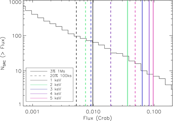
Figure 1. Log N–Log S plot obtained from the Swift-BAT 70 month hard X-ray survey. The vertical solid and dashed lines represent the source intensities corresponding to the MDP of 3% with 1 Ms exposure and MDP of 20% with 100 ks exposure, respectively. Different colors represent different threshold energies in the active scatterer.
Download figure:
Standard image High-resolution imageThe sensitivity of the polarimeter is generally given in terms of the Minimum Detectable Polarization (MDP) at the confidence level of 99% (Weisskopf et al. 2010), and is defined as

where, μ100 is the modulation factor for a 100% polarized beam. Rsrc and Rbkg are the source and background count rate, respectively, and T is the exposure time. The modulation factor, μ100, depends on the geometry of the Compton polarimeter and is typically in the range of 20% to 50%. The exposure time for the present generation polarimetric observations is of the order of 100 ks to 1 Ms. The dependence of MDP on the lower energy detection limit of the active scatterer comes from the source count rate, Rsrc; the lower the threshold, the higher the value of Rsrc, and the better the sensitivity is. The astrophysical significance of this dependence can be seen in Figure 1, which illustrates the number of X-ray sources accessible for the polarimetric investigation of the active scatterers different lower energy thresholds. This figure shows the log N–log S plot based on the Swift-BAT, hard X-ray catalog resulting from 70 months of observations (Baumgartner et al. 2013). There is a total of 1171 hard X-ray sources in the catalog, observed in the 14 keV to 195 keV energy band. This log N–log S plot is over plotted by the source intensities corresponding to the specified values of MDP, exposure time, and the lower energy threshold of the scatterer. These source intensities are computed using Equation (1) for different scatterer thresholds (1 keV, 2 keV, 3 keV, 4 keV, and 5 keV), assuming Crab-like spectra, and convolving the source spectra with the effective area of NuSTAR hard X-ray optics. The modulation factor, μ100, used here is obtained from our Geant4 simulations reported in Chattopadhyay et al. (2013). The vertical solid and dashed lines represent 3% MDP in 1 Ms and 20% MDP in 100 ks respectively, whereas different colors represent different scatterer thresholds. It can be seen that for lower thresholds, the number of observable sources available for the investigation of polarization, greater than a particular MDP, is significantly larger than that for higher thresholds. That is why, it is important to know the realistic threshold energy of the primary scatterer.
The plastic scatterer is not expected to have a sharp energy threshold because X-ray detection in the plastic scintillator is essentially a statistical process and it depends on various factors such as the location of the interaction, light collection efficiency, etc. Therefore, such a detector is likely to have a decreasing probability of low energy depositions in the plastic being recorded. Thus, for any Compton polarimeter design, it is very important to have an accurate understanding of the behavior of the active scatterer for low energy depositions in order to have a more realistic estimate of the polarimetric sensitivity.
In this context, we carried out a Compton scattering experiment that directly probes the behavior of the active scatterer for very low energy depositions. The experiment uses the same plastic scintillator configuration intended to be used in the Compton polarimeter. Here, we detect the Compton scattered X-rays using an independent detector at different scattering angles for an X-ray beam of known energy incident on the plastic scintillator along its axis. Recently, Fabiani et al. (2013) reported a similar study of the active scatterer based on the same concept. They concluded that the polarization measurements down to ∼20 keV are possible using the plastic scintillator as an active scatterer. However, their experimental setup was limited to a fixed geometry of the source, the scatterer and the absorber. We carried out a similar experiment, but with an improved experimental setup which allowed control over the scattering angle and thus the energy deposited in the scatterer, to investigate the response of the plastic scintillator at various deposited energies.
3. DESCRIPTION OF THE EXPERIMENT
3.1. Experiment Setup
Typically, the lower energy threshold for an X-ray detector is measured either by directly measuring low energy X-rays from a suitable monoenergetic X-ray source or by extrapolating the peak positions to energy relation to the noise floor of the detector. However, these methods are not suitable for our present objective for two reasons—(1) the energy resolution of the plastic scintillator is very poor and hence the extrapolation method cannot provide an accurate threshold, and (2) the encapsulation required for the scintillator prevents transmission of X-rays with energies less than ∼5 keV. For typical detector applications in such conditions, the transmission of the entrance window would determine the lower energy threshold. When the plastic scintillator is the scatterer for a Compton polarimeter, the energy range of interest for incident X-rays is >10 keV and hence the very thin entrance window of beryllium, as is typically used to achieve high window transmission, is not necessary. Here, the energy range of interest for detection of the deposited energy is ∼1–5 keV. Therefore, we employ the same principle of Compton scattering to investigate the response of the plastic detector to small energy deposition.
If a photon of energy E is Compton scattered at an angle θ, the energy deposited (recoil energy of electron) is given by,

where, mec2 is the electron rest mass. Figure 2 shows the variation of the deposited energy in the scatterer as a function of scattering angle for different energies of the incident photon. It can be seen that the incident photons with energies of ∼20–60 keV and scattered between 30°–150° angles, provide an opportunity for the investigation of the scatterer threshold within ∼0.5–10 keV.

Figure 2. Deposited energy in Compton scattering as a function of scattering angle and photon energy. Each line corresponds to a particular incident photon energy in keV as mentioned in the plot.
Download figure:
Standard image High-resolution imageIn the actual experiment, we detect the Compton scattered X-ray photons with energies of 59.5 keV and 22.2 keV (from radioactive sources 241Am and 109Cd, respectively), in the scattering angle range of 25°–140°, simultaneously with the trigger signal from the plastic scatterer. Figure 3 shows the experimental setup, which uses the plastic scatterer identical to the one that will be used in our planned configuration of the focal plane Compton polarimeter (Chattopadhyay et al. 2013). The scatterer is of 5 mm diameter and 100 mm length and is surrounded by a 1 mm thick aluminum cylinder and a 0.5 mm thick aluminum entrance window. It was obtained from Saint–Gobain as an integrated module containing plastic scintillator (BC404) coupled to a photo-multiplier tube (PMT; Hamamatsu R6095 with bialkali photocathode with maximum quantum efficiency of ∼25% at 420 nm). In the polarimeter configuration, the scatterer will be surrounded by a cylindrical array of CsI(Tl) scintillators, each of dimension 5 mm × 5 mm × 150 mm, to measure the azimuthal distribution of the scattered photons. In the present experiment, we are only interested in the polar scattering angle, and hence we use a small CdTe detector placed on a rotating arm. We used the standard X-123CdTe system from Amptek (Redus et al. 2006), which is kept on the rotating arm. The X-123CdTe is a compact integrated system consisting of a 1 mm thick CdTe (9 mm2 active area), pre-amplifier, digital pulse processor, MCA, and power supply. It also has a "gated" mode of operation, in which it accepts an event only if the gate is kept "ON" by applying a logic pulse. We use this mode to enforce the simultaneity between the plastic scatterer and the CdTe detector. As shown in Figure 3, the source photons from the radioactive source placed in front of the scatterer are scattered by plastic and the scattered photons are detected by the CdTe detector kept at a known angle. The positions of these two detectors can be adjusted in order to optimize the interaction location. A collimator (70 mm long with a 7 mm opening) made of Al is used in front of the CdTe window to localize the scattering region. The collimator is wrapped by a 1 mm thick lead to avoid contamination by any unwanted events. The FOV of the collimator is around 10°, which allows us to know the position of the interaction in the plastic scintillator within a few millimeters. It is crucial to maintain the alignment of the axes of the source aperture, plastic rod, and CdTe collimator to keep them in the same plane, and special care was taken to maintain the alignment at different scattering angles. In order to maximize the scattered counts in CdTe, a region at the top of the plastic was localized.
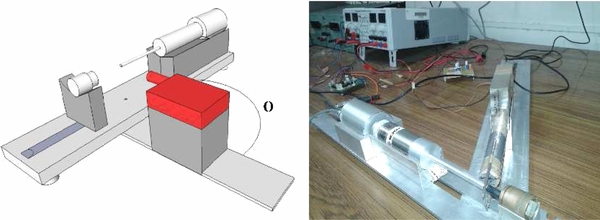
Figure 3. Left: schematic view of our experiment setup. Scattered photons from plastic are absorbed by CdTe kept at angle θ. Right: actual experiment setup—the axes of the plastic scintillator (along with PMT and CSPA), source, and CdTe are kept at the same plane using Al blocks. CdTe is kept on a rotating arm in order to detect photons at different scattering angles.
Download figure:
Standard image High-resolution imageWhen an incident photon deposits a sufficient amount of energy in the plastic scintillator, either by the photo-electric interaction or Compton scattering, a logic pulse with a fixed width of 3 μs is generated by the front-end electronics. The front-end electronics consist of CSPA, followed by a fast shaping amplifier (a unipolar-type with a shaping time constant of 2.6 μs) and a comparator as shown in the block schematic in Figure 4. The sensitivity of the scatterer also depends on the HV bias for the PMT and comparator threshold. During the initial trials, the optimum values for HV and comparator threshold were found to be 1 kV and 50 mV, respectively, and were then fixed for the entire experiment. The logic pulse generated by the front-end electronics was then fed to the input of the X123CdTe systems "Gate" and thus it detected the photons only for the duration of 3 μs following a trigger from the plastic scatterer. For each scattering angle, we acquired two sets of spectra from CdTe—first, with the coincidence between CdTe and plastic enforced, which actually gives the Compton scattering events, and second, without coincidence (PMT HV off), i.e., plastic behaving as a passive scatterer. With the simultaneity between plastic and CdTe enforced, it is expected that only a very small fraction of all the triggers would have simultaneous detection in the CdTe and hence the total experiment duration has to be very large (a few hours) but would result in a relatively very short acquisition time of a few minutes. This has important implications in our semianalytical modeling as discussed in the following sections.

Figure 4. Block schematic for the coincidence unit between plastic scintillator and X123CdTe.
Download figure:
Standard image High-resolution image3.2. Results
The spectra acquired from the CdTe detector at three different scattering angles in both the modes, i.e., in coincidence with the scatterer and without coincidence, for both 59.5 keV (from 241Am) and 22.2 keV (from 109Cd) incident X-rays are shown in Figure 5. These spectra are normalized with respect to actual acquisition time (time for which the CdTe "Gate" was on during the exposure). In each plot, the solid line represents spectrum in coincidence mode and the dashed line represents spectrum in noncoincidence mode. The backgrounds in both coincidence and noncoincidence mode are negligible compared to the respective source counts. It can be seen that the count rate in the coincidence mode is higher than that in the noncoincidence mode, as expected, because in coincidence mode, the CdTe detector accepts an event only for a short duration after each trigger in the plastic scatterer. The energy of the Compton peaks also changes with scattering angle, as expected. The detection of Compton peak at 60° from 22.2 keV X-rays clearly shows that the plastic scatterer can detect energy depositions less than 1 keV. Figure 6 shows the observed count rate at all measured angles for both the sources. Total counts for the 241Am are obtained by summing over ±3 FWHM from the peak energy for each spectrum, however, for the 109Cd, total counts are obtained by summing over −3 FWHM to +1 FWHM in order to avoid contribution from the secondary peak at 25 keV. Again, for each spectrum, the count rate is with respect to the actual acquisition time which is related to the exposure time by equation

where, Tco (∼200 s for Am241 and ∼100 s for Cd109) and  (∼2 hr for Am241 and ∼7 hr for Cd109) are acquisition time and exposure time, respectively, in coincidence condition; Rtrig is trigger rate in plastic and Twin is the coincidence time window (∼3 μs). The acquisition time is measured by the CdTe detector, which allows one to calculate trigger rate for each measurement.

Figure 5. Coincidence (solid) and noncoincidence (dashed) spectra observed with the CdTe detector at different scattering angles. Upper panel (left to right) shows spectra for 59.5 keV from 241Am at scattering angles 140°, 90°, 35° respectively. Lower panel (left to right) shows spectra for 22.2 keV of 109Cd at scattering angles 140°, 90°, 60° respectively. Energy of primary incident photons have been represented by the dotted lines.
Download figure:
Standard image High-resolution image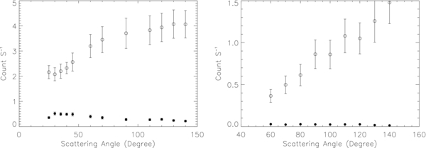
Figure 6. Observed count rate for 59.5 keV (left) and 22.2 keV (right) for coincidence (open circles) and noncoincidence (filled circles) modes as a function of scattering angles.
Download figure:
Standard image High-resolution imageThe count rates in coincidence mode, Rco, and in noncoincidence mode, Rnco, are given by


where Nco and Nnco are the summed counts under these peaks (Compton and Rayleigh) in coincidence and noncoincidence mode, respectively, for a particular angular position, θ, of CdTe. Tnco (0.5 hr for 241Am and 1.5 hr for 109Cd) is the acquisition time in noncoincidence mode.
Since, Tco ≪ Tnco, Rco ≫ Rnco, as can be seen in the figure with open circles and filled circles representing coincidence and noncoincidence modes, respectively. At lower angles (<45°), there is also a finite probability of the source photons directly entering into the CdTe detector, which leads to an increase in count rate in both noncoincidence and coincidence mode due to the chance coincidences. This problem is only present for the 241Am source, because in the case of 109Cd, the measurements are limited to scattering up to 60°. To correct for the spurious count rate due to direct exposure, we measured the number of counts at lower angles for 241Am without having the plastic scintillator in place. This configuration then measures any "leakage" of photons through the intervening material. However, direct subtraction of these counts from the observed counts for 241Am at the respective lower angles would underestimate the noncoincidence count rate because the plastic scintillator and the surrounding aluminum may absorb some of these photons. We estimated this absorption fraction for different angles at energy 59.54 keV based on the geometry of our experiment setup. The observed count rate due to direct exposure (without the plastic scatterer) is then corrected by this absorption fraction and then subtracted from the observed count rate (with the plastic scatterer) to calculate correct count rate due to scattering only.
The error bars shown here combine both statistical and systematic uncertainties. The sources of systematics are misalignment between collimator and plastic scatterer, uncertainty in angle measurement, uncertainty in the center of rotation of CdTe around plastic, and uncertainty in the coincidence time window. The most prominent source of error is the misalignment of plastic and the collimator, for which we have tried to control within the experimental limits. The contributions of each of these sources to overall systematic error is estimated as per following discussion. Error due to misalignment between plastic axis and CdTe collimator axis is obtained by geometrically estimating the intersection area of the CdTe field of view with the plastic for a given angle. A misalignment of 1 mm introduces a minimum of 9% error across all the angles; contribution is maximum (∼14%) for angles close to 90° and minimum for lower scattering angles (∼9%). Error due to uncertainty in angle measurement is computed by estimating the change in the Compton and Rayleigh scattering cross-section and is found to be less than 0.1% at angles close to 90° and about 1% at other angles for an angle measurement uncertainty of 1°. Error due to uncertainty in the coincidence time window is directly proportional to the amount of uncertainty present and its value is found to be 6% for uncertainty of 0.2 μs. Uncertainty in the central position of interaction reflects change in transmission probability of photons. Contribution of this is found to be of the order of 2% for 59.54 keV and 4% for 22.2 keV. Systematic errors are therefore angle dependent. We estimated combined systematic uncertainties to be 10% at lower and higher scattering angles and 16% at angles close to 90°. These are added to the statistical uncertainties in quadrature. Each measurement has been repeated several times to have confidence in the observed count rates and we have considered average count rates from multiple measurements where necessary.
Figure 6 shows that, at higher angles the coincidence count rate is more than that in the noncoincidence count rate because of large energy deposition, which is above the threshold. As we move toward the lower scattering angles, because of lower energy deposition, the fraction of valid Compton scattered photons decreases and consequently the coincidence and noncoincidence count rates tend to match each other. Thus, this figure demonstrates the essence of our experiment in qualitative terms—that although the plastic scatterer is able to detect energy deposition as low as ∼1 keV, the efficiency of detection decreases gradually with decreasing energy.
However, these representations of count rate versus scattering angles are not suitable for quantitative estimation of detection efficiency as a function of deposited energy in the scatterer due to the fact that the trigger rate in the plastic scatterer is not constant across all the scattering angles. In order to minimize the total exposure times, particularly in the coincidence mode, it is necessary to keep the source as close as possible from the scatterer. However, this distance is different for different scattering angles, which results in variation of the total trigger rate (i.e., total interactions including photo-electric and detectable Compton scattering interactions) in the plastic scatterer.
Therefore, it is necessary to normalize count rates with respect to the number of triggers in plastic. If Rtrig is the trigger rate in plastic for angle θ (obtained from Equation (3)), then normalized count rates, i.e., the number counts in the CdTe detector per trigger in the plastic scatterer, at θ are given by


Denominator in Equations (6) and (7) is the total number of triggers in plastic during the experiment. Figure 7 shows the normalized rates in coincidence and noncoincidence modes for both sources. Since,  ≫
≫  , the normalized rate in noncoincidence mode, represented by filled circles, is much higher than that in the coincidence mode, denoted by open circles. Since, statistical error on count rate is inversely proportional to exposure time, error in noncoincidence mode is larger too. We see that count rate in coincidence mode is decreasing in a steady manner. This clearly shows that the plastic scatterer does not have a sharp detection threshold, rather, the detection efficiency gradually decreases with decreasing deposited energy.

Figure 7. Normalized count rate with respect to the total number of triggers in plastic (see the text for further details) for 59.5 keV (left) and 22.2 keV (right) as a function of scattering angles. Open and filled circles stand for coincidence and noncoincidence modes, respectively.
Download figure:
Standard image High-resolution imageIt can be seen that the normalized count rate in noncoincidence mode is always greater than that in coincidence mode. For 241Am, X-rays scattered at large scattering angles, the energy deposited in the scatterer is more than ∼5 keV, which is always expected to generate a trigger in the scatterer. Thus, it is expected that in this range the normalized rate in both noncoincidence and coincidence mode should be the same, due to much smaller probability of the Rayleigh scattering at this energy. However, the fact that the observed normalized count rate in noncoincidence mode is higher than that in coincidence mode, suggests that the scattering events taking place in the material apart from the plastic scintillator, e.g., the surrounding Aluminum cylinder, because of the diverging beam, also contribute to the noncoincidence count rate. In coincidence mode, these events get suppressed due to the requirement of the simultaneity. This further suggests that the contribution of such events must be taken into account while estimating the number of chance coincidence events in the coincidence mode as well.
4. NUMERICAL MODELING
Figure 7 presents the number of scattered photons detected by the CdTe detector at a given scattering angle for each trigger registered in the plastic scatterer. Since the scattering geometry of our experiment is fairly simple, in principle, it should be possible to estimate this count rate using the knowledge of the Compton scattering cross-section of the plastic scatterer. However, we find that such a simple minded calculation does not give count rate estimation or the trend of its variation with scattering angle, which can be directly compared with the observed results. On further investigation, we find that it is essential to consider various factors such as
- 1.The finite scattering length as viewed by the CdTe detector through collimator.
- 2.Absorption of the incident photons by the entrance window in front of the plastic scatterer.
- 3.Absorption of the photons scattered from the plastic scatterer in the surrounding aluminum.
- 4.Scattering of incident photons from the surrounding aluminum itself.
- 5.Multiple-scattering within plastic and aluminum.
- 6.Efficiency of CdTe at the scattered energies
- 7.Scattering of photons from inner aluminium surface of the collimator.
We attempted to model the observed results including most of these factors.
We start with Klein Nishina cross-section (Heitler 1954) for Compton scattering

where E and E' are energies of incident and scattered photon, respectively, for scattering angle, θ. From Equation (8), one can obtain Thomson scattering cross-section by substituting E = E'
Here, we assume that the photons from the source are being scattered by plastic along its axis. For a given angle θ, range in angle of scattering and the scattering length are calculated from the known geometry (see Figure 8). Then, we divide the scattering length into a large number of small segments and for each segment, both polar and azimuthal scattering ranges, i.e., θmin, i, θmax, i and ϕmin, i, ϕmax, i subtended by the CdTe detector at the center of the ith segment, are calculated. The cross-section of each segment for a photon to be scattered in the direction of the CdTe detector is then estimated by integrating Equations (8) and (9) over these angle ranges.

For integration over ϕ for the ith segment, we estimated ϕmin and ϕmax at both the θmin position and θmax position and took the average of ϕmin and the average of ϕmax as limit of integration.
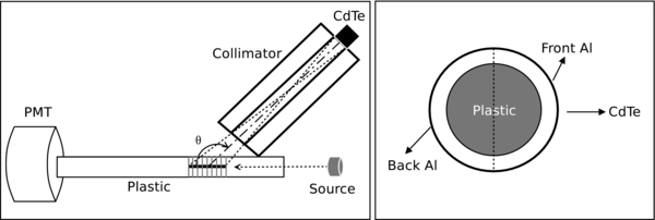
Figure 8. Left: geometric representation of the experimental setup. In the model, the total length of the plastic scatterer observed by the CdTe detector is calculated based on this geometry which is then further divided into a large number of small segments as shown by the grey parallel lines. Right: front surface of the plastic (5 mm diameter). The plastic is surrounded by 1 mm thick Al. The Al surface facing the CdTe is named as front Al and the opposite surface as back Al.
Download figure:
Standard image High-resolution imageOne important point to be noted here is that the cross-sections in Equations (8) and (9) are valid for the scattering of free electrons. However, in case of realistic matters, the binding effect of electrons and their momentum distributions inside the atom introduce significant difference in the scattering distribution especially at the lower angles. Thus, the numerical values obtained from Equations (10) and (11) are expected to differ from the actual true values because of these effects. This point is specifically discussed in Muleri & Campana (2012). Though forward scattering is not dominant in our experiment, we accounted for these effects by considering more realistic scattering cross-sections, including atomic form factors and incoherent scattering functions into the calculations for the scattering atom under consideration as shown below.
where,

S(x, Z) and F(x, Z) are the incoherent scattering functions and atomic form Factors, respectively, for element of atomic number Z. The values of S(x, Z) and F(x, Z) as a function of x are obtained from Hubbell et al. (1975). For a given incident photon energy, (E), it is possible to get these values as a function of scattering angle which typically ranges from 0° to 160°. For our purpose, we interpolated the form factor and scattering functions at each degree and used them in Equations (12) and (13). Since plastic is a compound material consisting of H and C atoms, form factors and scattering functions for plastic have been computed by taking proper weight factors into their individual form factors and scattering functions.
Dividing Equations (12) and (13) by total Compton and Rayleigh cross-section for the ith section, respectively, we get the probability of photons scattered by the ith segment, reaching the CdTe detector, kept at angle θ


where PC(θ, i) and PR(θ, i) are the fractions of total scattered photons by the ith segment that reach CdTe. Total cross-sections have also been computed in a similar fashion by taking into account form factors and scattering functions.
To get the total number of Compton and Rayleigh scattered photons reaching the CdTe detector, it is necessary to multiply PC(θ, i) and PR(θ, i) by the probability of respective interaction taking place in the ith segment. This probability is calculated using the mass attenuation coefficients of Compton and Rayleigh scattering for the plastic scintillator obtained from the NIST database (Berger & Hubbell 1987).
If the ith segment has thickness "Sp" ("p" stands for plastic), then the fraction of photons Compton scattered by that segment is ![${\mu ^p_c }/{\mu ^p_t} [1 - \mathrm{e}^{-\mu ^p_t \rho _p s_p}]$](https://content.cld.iop.org/journals/0067-0049/212/1/12/revision1/apjs493694ieqn4.gif) and the fraction of photons Rayleigh scattered is
and the fraction of photons Rayleigh scattered is ![${\mu ^p_r }/{\mu ^p_t} [1 - \mathrm{e}^{-\mu ^p_t \rho _p s_p}]$](https://content.cld.iop.org/journals/0067-0049/212/1/12/revision1/apjs493694ieqn5.gif) . Here,
. Here,  ,
,  , and
, and  are respectively the Compton, Rayleigh scattering attenuation coefficient and total attenuation coefficient of plastic at the incident photon energy, E. ρp is the density of plastic. Therefore, fraction of incident photons detected by CdTe at angle θ is given by
Summation is performed over all the segments (each of thickness "Sp") in plastic. N is the total number of segments.  refers to photons incident on plastic. The exponential term,
  , takes into account the transmission through a thin window made of plastic (thickness, tw = 3 mm; density, ρw; total absorption coefficient at E, μw) at the front of plastic scintillator. The first and second part in Equation (17) stands for Compton and Rayleigh events in plastic, respectively. We have assumed the 100% detection efficiency of CdTe which is a good approximation, as for 1 mm CdTe efficiency falls from 100% beyond 60 keV.
A fraction of these scattered photons will be absorbed by the surrounding front Al (see Figure 8) of thickness 1 mm. However, the photon path length (absorption thickness) depends on the scattering angle. The absorption coefficient of Al also depends on the scattered energy. Hence, both these factors will vary from segment to segment. For simplicity in calculation, we estimated the photon path length corresponding to the mean of minimum and maximum scattering angle for each segment. The absorption coefficient is also evaluated at energy corresponding to that mean scattering angle. The angle range being very small, this approximation holds true. If tfa and  (E' is the scattered energy corresponding to mean scattering angle) are the absorption thickness and total absorption coefficient of front Al for the ith segment, then absorption factor is given by
  , where ρa is the density of Al and "fa" stands for front Al. With the inclusion of this factor, Equation (17) is modified to

where, first (Compton) and second term (Rayleigh) are given by

It is to be noted here that the attenuation coefficients of aluminum need to be taken at respective energies of the photon, i.e., for Compton scattering it is the energy of the scattered photon and for Rayleigh scattering it is the energy of the incident photon.
As discussed earlier, it is essential to consider scattering from the aluminum cylinder surrounding the plastic scatterer. Keeping the source opening and source-plastic distance in mind, it is assumed that radiation is uniform over the plastic and surrounding Al. We estimated the contribution in scattered photons from both front Al and back Al (see Figure 8) with the same approach mentioned above. It is assumed that the photons are scattered along the axes of front and back Al and the angles of scattering have been calculated with respect to these axes. Therefore, the scattering angle range for any segment is different for different scatterers, i.e., plastic, front Al and back Al. The fraction of photons scattered by front and back Al at angle θ is given by

where  and
and  are the incident photons on front Al and back Al, respectively. Other symbols have their meaning as described earlier. It is to be noted that in Equation (21), the absorption terms have been dropped because there is no source of absorption for photons scattered from front Al. However, the photons scattered from back Al will suffer absorption from the 5 mm plastic and the 1 mm front Al. These factors have been included in Equation (22).
Now, assuming uniform exposure of the incident X-rays over the plastic scatterer and surrounding aluminum, it can be shown that if  is the number of photons incident on plastic, then the number of photons incident on front and back Al are, respectively,
  and
and  (diameter of plastic is 5 mm and diameter of plastic plus Al is 7 mm). Therefore, using Equations (18), (21), and (22), one can obtain the ratio of photons scattered into CdTe at angle θ to the number of photons incident on plastic as

The normalized count rate shown in Figure 7, as defined in Equation (7), is the ratio of number of scattered photons detected by the CdTe detector to the total number of triggers in the plastic scatterer, hereas Equation (23) gives the ratio of number of scattered photons likely to be detected by the CdTe detector to the total number of incident photons on plastic of the given energy, i.e., either 59.5 keV or 22.2 keV. These two ratios cannot be compared directly due to the fact that both 241Am and 109Cd sources emit photons of multiple energies and thus all triggers generated by the plastic scatterer included those generated by incident photons having energies other than that of interest. Here, again it is possible to modify the ratio given by Equation (23) based on the knowledge of the relative intensities of different lines emitted by both sources. However, exact values of relative intensities of the X-ray lines capable of generating triggers in the plastic scatterer are not available for the sources we have used during the experiment. Also, exact calculation of this ratio would require the assumption of 100% trigger generation efficiency at all energies. Therefore, instead of calculating the ratio of incident photons to the triggers in the plastic scatterer, we modify Equation (23) to include a fit parameter, α, representing this ratio. This parameter also takes into account any small deviations from the strict alignments of source to scatterer and scatterer to CdTe axis, as assumed in the model, provided that the deviation is constant across all angles. Thus, the final expression of the model is given by

Therefore, to quantitatively compare the observed results with expected values, we fit Equation (24) to the results shown in Figure 7 and obtain the best fit value of the parameter, α, by χ2 minimization.
5. MODELING RESULTS AND DISCUSSIONS
Figure 9 shows the fitted model (thick solid line, Equation (24)) with the experimental results. For 241Am, the best fit value for parameter α is 3.65, whereas for 109Cd, it is 0.88. These values are reasonably close to the values expected from the available data for relative intensities of different X-ray lines for both 241Am and 109Cd sources. Different components of the model are shown in Figure 9: Compton scattering events from plastic (dashed, Equation (19)), Rayleigh scattering events from plastic (dotted, Equation (20)), combined Compton and Rayleigh events from plastic (thin solid, 1st term of Equation (24)), and scattering events (Compton + Rayleigh) from front Al (dashed dot dot, 2nd term of Equation (24)) and back Al (long dashed, 3rd term of Equation (24)) surrounding the plastic.

Figure 9. Observed count rate in the noncoincidence mode fitted by the model. The left plot corresponds to 59.5 keV and the right plot corresponds to 22.2 keV photons. The thick solid line represents final model (Equation (24)) whereas the thin lines represent different components of the model—dashed lines: Compton scattering events from plastic; dotted lines: Rayleigh scattering events from plastic; solid lines: sum of Compton and Rayleigh events from plastic; dashed dotted lines: scattering events from front Al; long dashed lines: scattering events from back Al. Best fit values of the parameter of the fitted curve are 3.65 and 0.88 for 59.5 keV and 22.2 keV, respectively.
Download figure:
Standard image High-resolution imageThus far, this model is aimed at reproducing the observed count rate in the noncoincidence mode, i.e., the scatterer is considered to be passive. The observed count rate in the coincidence mode can be estimated from Equation (19) along with the chance coincidence rate due to all other terms, i.e., Rayleigh scattering in the plastic scatterer (Equation (20)), scattering from the aluminum cylinder (second and third terms of Equation (24)) as well as chance coincidence of the real Compton scattering events which failed to generate trigger. The chance coincidence fraction of these terms can be given by the product of trigger rate in the plastic scatterer and the width of the coincidence window, i.e.,

where, fch is the chance coincidence factor. Thus, the total expected count rate in the coincidence mode can be expressed as
where, α is the best fit parameter obtained from fitting the noncoincidence mode data. The Compton scattering term is multiplied by the energy dependent probability of generating trigger in the plastic scatterer for given energy deposition. All the terms in this equation, except the detection probability, P(E), can be estimated using Equations (6), (18), (21), and (22). Comparison of the expected count rate from Equation (26), assuming the detection probability to 100%, with the observed count rate in the coincidence mode is shown in Figure 10. We see that at higher scattering angles for 241Am, modeled and experimental coincidence count rates agree well with each other, implying 100% detection probability at those energies. At lower angles for both the sources, experimental values are significantly less than the model values, indicating lower detection probability at lower energies. This probability can be determined directly by comparing model values with the observed values and are shown in Figure 11 for both 241Am (represented by open triangles) and 109Cd (represented by filled triangles) sources. Here, the X-axes are converted from the scattering angles into the deposited energies corresponding to the scattering of incident photons (59.5 keV and 22.2 keV) at those angles. Figure 12 shows combined data from both the sources as uniformly increasing trigger generation efficiency of the plastic scatterer in the energy range of 0.4–10 keV. It can be seen that there is a common energy range of 0.65–1.55 keV in the energy depositions by both sources, corresponding to small angle scattering of 59.5 keV photons and large angle scattering of 22.2 keV photons, and the observed values for both the sources agree well with each other. The small angle scattering of 22.2 keV photons gives ∼6% detection efficiency at energies down to ∼0.5 keV, which then increases almost linearly up to 3.0 keV. At energies greater than 7 keV, the detection efficiency almost saturates at 100%, as expected. The observed variation of detection efficiency can be fitted by an empirical polynomial given in Equation (27).

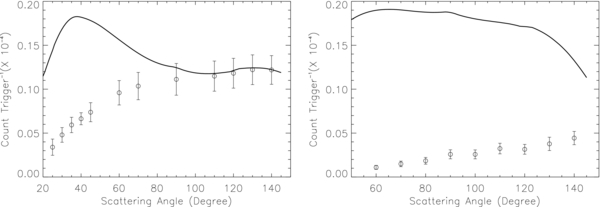
Figure 10. Comparison between experimentally obtained coincidence count rate and modeled count rate, assuming 100% detection probability of plastic. The left plot shows the comparison for 59.5 keV. The right plot shows the comparison for 22.2 keV.
Download figure:
Standard image High-resolution image
Figure 11. Detection probability of the plastic scintillator as the function of deposited energy in plastic. Left: probability of event detection obtained from 59.5 keV photons. Right: detection probability estimated from 22.2 keV.
Download figure:
Standard image High-resolution image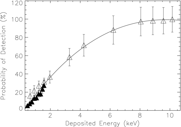
Figure 12. Detection probability as a function of deposited energy from 0.4 keV to 10 keV. Filled and open triangles correspond to 22.2 keV and 59.5 keV photons, respectively. These data points have been fitted with an empirical polynomial shown by the solid line.
Download figure:
Standard image High-resolution imageIt is important to note a few points regarding our modeling. (1) This expression for the variation of detection efficiency as a function of energy depends on other experimental factors such as HV bias for the PMT and comparator threshold of the front-end electronics as well as the specific configuration of the plastic scatterer and its encapsulation. However, our modeling does not depend on these factors as the model fitting is with respect to the observations in the noncoincidence mode. Thus, any further optimization of the experimental factors would only influence the observed count rate in coincidence mode and thus would automatically result in better detection efficiency from the same model. (2) This expression represents the worst case scenario in terms of the interaction position within the plastic scatterer because in our present experiment only the interactions within the top couple of centimeters of the plastic scatterer are considered. For deeper interactions, the trigger generation efficiency may be slightly better due to reduced light path, but surely not worse than the present case. (3) This empirical expression is valid for our configuration of the plastic scatterer (e.g., 10 cm long and 5 mm diameter BC404). Though the general trend is expected to be same for any other configuration, the exact expression must be measured separately.
Now that we have an empirical expression representing the detection efficiency for our configuration of the plastic scatterer, we can use that to estimate the sensitivity of the Compton polarimeter more accurately. In our earlier simulation studies (Chattopadhyay et al. 2013), we investigated the sensitivity of a hard X-ray focal plane Compton polarimeter comprising the same configuration of the plastic scatterer and coupled with the NuSTAR type of hard X-ray optics. The MDP of this configuration of polarimeter was found to be 0.9% in 1 Ms for a 100 mCrab source, when the threshold for the scatterer was assumed to be 1 keV. The MDP for the threshold of 2 keV was found to be 1.2% for the same conditions. We reanalyzed the data from the same simulations using the above expression for energy dependent detection efficiency (see Equation (27)) of the plastic scatterer and the results are shown in Figure 13. It can be seen that the MDP for the same conditions (1 Ms exposure for 100 mCrab source) is 1.2%, indicating slightly degraded, but more realistic, sensitivity. The lower energy limit for the polarization measurement is also improved to ∼14 keV due to the finite probability of detecting energy depositions as low as ∼0.5 keV by the plastic scatterer. However, it should be noted that at energies less than ∼20 keV, the properties of the material between the scatterer and the absorber, in our case 1 mm and 0.5 mm aluminum surrounding the scatterer and in front of the absorber, respectively, become very important as the scattered photon has to pass through it without undergoing any further interaction. We attempted to replace the aluminum by lower-Z materials in our simulations, but the results were not very encouraging due to the enhanced scattering in the intervening low-Z material, which degraded the overall modulation pattern of the scattered photons. Thus, we find that in order to improve the sensitivity as well as overall efficiency of the Compton polarimeter, apart from the obvious optimization of the plastic scatterer configuration and associated electronics, it is equally important that the material between the scatterer and the absorbers has a higher atomic number to reduce scattering, and is as thin and uniform as possible to enhance the transmission of the photons scattered from the central scatterer. Overall, we find that polarization measurements down to ∼15 keV are certainly possible using Compton polarimeter. Since many celestial sources are expected to have energy dependent X-ray polarization signatures, it is important to take into account the detection efficiencies of the active scatterer, especially at the lower energies, while interpreting the eventual energy integrated polarization measurements.

Figure 13. MDP as a function of source intensity. The triangles and asterisks stand for 1 Ms and 100 ks exposure, respectively. Solid lines refer to the single NuSTAR collecting area of mirror. Dashed lines refer to five times the NuSTAR mirror area. Different background rates have been denoted by thick and thin lines. For bright sources, MDP is below 1%. However, it is to be noted that eventual polarization sensitivity will be limited by systematics of the instrument.
Download figure:
Standard image High-resolution image
6. CONCLUSIONS
The sensitivity and energy range of any Compton polarimeter critically depend on the response of the active scatterer to very low energy deposition. Since the plastic scintillators are the scatterer of choice for Compton polarimeter, it is important to understand their behavior for low energy deposition. However, it is difficult to characterize a plastic scintillator using usual spectroscopic methods. Therefore, we carried out an experiment to investigate the characteristics of a 10 cm long and 5 mm diameter plastic scatterer using the principle of Compton scattering. Here, we have presented the experimentally measured detection efficiency of the plastic scatterer in the energy range of 0.5–10 keV. We have also substantiated our experimental results using semianalytical modeling of our experimental setup. We find that the detection efficiency of the plastic scatterer is 100% for energy deposition greater than ∼7 keV and gradually decreases for lower energy deposition. For energy deposition of 1 keV, the detection efficiency is found to be ∼17%–18%. The sensitivity and energy range of a Compton polarimeter are typically estimated by assuming a sharp energy threshold for the active scatterer. However, this study shows that such an assumption is not true for a plastic scatterer and the actual energy dependent detection efficiency of such a scatterer must be taken into account.
The research work at Physical Research Laboratory is funded by the Department of Space, Government of India.