


ABSTRACT
The ζ Aurigae system 31 Cygni (K4 Ib + B4 V) was observed by the FUSE satellite during total eclipse and at three phases during chromospheric eclipse. We present the coadded, calibrated spectra and atlases with line identifications. During total eclipse, emission from high ionization states (e.g., Fe iii and Cr iii) shows asymmetric profiles redshifted from the systemic velocity, while emission from lower ionization states (e.g., Fe ii and O i) appears more symmetric and is centered closer to the systemic velocity. Absorption from neutral and singly ionized elements is detected during chromospheric eclipse. Late in chromospheric eclipse, absorption from the K star wind is detected at a terminal velocity of ∼80 km s−1. These atlases will be useful for interpreting the far-UV spectra of other ζ Aur systems, as the observed FUSE spectra of 32 Cyg, KQ Pup, and VV Cep during chromospheric eclipse resemble that of 31 Cyg.
Export citation and abstract BibTeX RIS
1. INTRODUCTION
The ζ Aurigae stars are eclipsing binary systems consisting of a cool giant or supergiant with a hotter main-sequence companion. As the hot star enters into and exits from eclipse, its light shines through the cool star chromosphere and wind. The orbital motion provides a probe of the spatial structure of the cool star chromosphere and wind acceleration region. Among these binaries, 31 Cygni (K4 Ib + B4 V) is especially well-suited for this mapping, as the binary components are separated far enough to minimize interaction, producing a less complex spectrum than is observed for similar systems like VV Cep.
The region of the ultraviolet spectrum of 31 Cyg accessible to IUE has been well observed. Bauer & Stencel (1989) identified the spectral features, and chromospheric models have been produced by Eaton (1993, 2008) and Eaton & Bell (1994).
The FUSE satellite opened up observations of the ζ Aur stars to shorter wavelengths. 31 Cyg was observed with The FUSE program D123 (PI: Bennett) in 2003 during total eclipse at two epochs during fairly deep chromospheric eclipse and at one epoch at which only weak chromospheric lines were seen. The ultraviolet spectrum of this binary was also observed far from eclipse with Hubble Space Telescope (HST) in 2001 and 2002. Figure 1 shows the relative orbit of the two stars as calculated from the orbital solution of Wright (1970) for the K-type supergiant and the velocity semi-amplitude K2 of Eaton (1993) for the B-type companion. The position of the B star is shown at the epochs of the FUSE and HST observations. During total eclipse, an emission spectrum due to scattering of B-star photons in the wind is observed (Bennett 2006). Outside of total eclipse, an absorption spectrum is seen as the B-star continuum shines through the chromosphere and wind of the K star. Interstellar absorption from H2 molecules and zero-volt lines of atomic species is also observed.
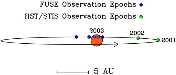
Figure 1. Relative orbit of 31 Cyg.
Download figure:
Standard image High-resolution imageIn this paper, we derive coadded, calibrated FUSE spectra for the observations and present these results in the form of a far-ultraviolet (far-UV) spectral atlas, with line identifications produced using the Hirata & Horaguchi (1995) compilation of atomic data.
2. OBSERVATIONS
The FUSE satellite covered the wavelength range 900–1190 Å. Four separate "channels" (optical paths) used two mirrors coated with SiC and two with LiF, optimizing sensitivity at shorter and longer wavelengths, respectively. There were two detectors, leading to eight individual spectral segments. The wavelength and flux calibrations of each of the segments depended on how well centered the target was in the aperture. Simultaneous alignment of all channels was an ongoing and challenging problem for the FUSE satellite because of mechanical flexure of the optical train due to variations in the spacecraft thermal environment with attitude. Generally, alignment of the SiC channels (and therefore, observing with these channels) was only feasible through the large (LWRS) aperture. At the time of our observations, the fine error sensor (FES-A) guide camera was tied to the LiF1 channel; the default guide camera was subsequently changed to FES-B, linked to LiF2, in 2005 July (Andersson 2006).
The seven observations made of the 31 Cygni system by the FUSE satellite are listed in Table 1. Orbital phases were computed from the orbital solution of Wright (1970). The first two observations were safety snaps (SAFTSNPs) made to avoid an overexposure. Although the first one (D1230201) is quite underexposed, it samples chromospheric eclipse at a time it would not otherwise have been observed, and contains useful information. The second safety snap (D1230202) was made during total eclipse. Since totality was covered by two additional well-exposed observations, this observation is listed here only for completeness. The well-exposed total eclipse observations, D1230203 and D1230204, were made through the large LWRS aperture. The lines of the N ii UV multiplet 1 near 1085 Å were brighter in eclipse than expected, with a peak flux of 8.0 × 10⁻¹¹ erg cm−2 s−1 Å−1 (making these the brightest lines in these FUSE eclipse spectra of 31 Cyg). Consequently, the FUSE Science Operations team, worried about the possibility of dangerously bright out-of-eclipse fluxes, required all subsequent observations with the (more sensitive) LiF channels to use the smallest (HIRS) aperture, which transmits only ∼85% of the incident flux. Since simultaneous observations with the SiC channels are not possible using the HIRS aperture, this restriction meant that only the longer wavelength portion of the FUSE range could be observed in a single observation. Observations at shorter wavelengths could still be done using the (less sensitive) SiC channels through the LWRS aperture, but these would now require a separate observation. Therefore, the three further planned sets of post-eclipse observations with full spectral coverage were reduced to two post-eclipse visits, only one of which had full spectral coverage. The observation immediately following totality (D1230205) only observed chromospheric eclipse in the LiF channels. The remaining visit, about three months later, observed both the long-wavelength LiF channels (D1230206) and the short-wavelength SiC channels (D1230207) as two separate observations.
Table 1. FUSE Observations of 31 Cygni
| Observation | Aperture | UT | Phase | Exposure | Comments |
|---|---|---|---|---|---|
| Date | Time (s) | ||||
| D1230201 | LWRS | 2003 May 23 | 0.9893 | 58 | SAFTSNP – ingress, deep chromospheric eclipse |
| D1230202 | LWRS | 2003 Jun 20 | 0.9969 | 58 | SAFTSNP – total eclipse |
| D1230203 | LWRS | 2003 Jun 30 | 0.9996 | 3169 | Total eclipse |
| D1230204 | LWRS | 2003 Jul 18 | 0.0042 | 3936 | Total eclipse |
| D1230205 | HIRS | 2003 Aug 23 | 0.0138 | 1451 | Egress, deep chromospheric eclipse |
| D1230206 | HIRS | 2003 Nov 20 | 0.0373 | 1640 | Egress, late chromospheric eclipse |
| D1230207 | LWRS | 2003 Nov 20 | 0.0374 | 872 | Egress, late chromospheric eclipse |
Download table as: ASCIITypeset image
3. DATA CALIBRATION AND REDUCTION
The star 31 Cygni is so bright in the far-UV that it was necessary to carry out FUSE observations in HIST mode, for which information about individual photons is not retained, which limits the post-observation processing that can be done. The CalFUSE pipeline returned reduced, calibrated FITS data files for each of the several exposures made during each observation. (Observations had been divided into several exposures by the FUSE data acquisition system to minimize orbital Doppler smearing.) The individual exposures produced by CalFUSE were subsequently (by the authors) cross-correlated in velocity and coadded to produce a final flux-calibrated spectrum for each detector segment.
The FUSE detectors have a complex optical configuration, resulting in a total effective area that depends strongly upon wavelength. The lack of an onboard wavelength calibration lamp makes it necessary for users to calibrate their science exposures, usually using interstellar lines. However, thermal flexure and misalignment problems mean that these wavelength and flux calibrations are not reproducible from observation to observation. There is substantial redundancy in the full set of FUSE observations when all eight detector channels are aligned. To make full use of a science exposure, it is desirable to combine these eight individual spectra into one coadded result, especially for the production of a spectral atlas. This is not a trivial task.
Interstellar lines from H2 molecules and various atomic species appear abundantly in the FUSE spectrum of 31 Cyg and provide a convenient velocity reference at shorter wavelengths (λ < 1153 Å). However, no interstellar features appear in the FUSE spectrum of 31 Cyg at longer wavelengths, and that presented a problem for the wavelength calibration of some observations. Before any calibration could be carried out, it was necessary to establish the velocity scale of the interstellar lines, and this was done by comparison to HST observations. 31 Cyg was observed with the STIS ultraviolet spectrograph at a high resolution using echelle modes E230H & E140H by GO program 9109 (PI: Bennett) at two epochs near quadrature in 2001 November and 2002 August. For this work, we used the StarCAT reduction of Ayres (2010). Weak interstellar features showed up to four sharp individual components. These components blended into a single feature as the lines strengthened. IUE spectra of 31 Cygni at similar phases were compared to the HST spectra, and only the blended features were detected at the lower resolution of IUE. None of the interstellar lines resolved by FUSE showed multiple components. Therefore, observed wavelengths were measured in the HST data for those interstellar lines strong enough to show the single blended feature. A total of 16 lines were measured (10 lines from one exposure and 6 from the other, which had less wavelength coverage) and the average radial velocity was −16.1 ± 0.8 km s−1.
Therefore, the rest wavelengths of interstellar atomic and H2 molecular lines seen in the FUSE spectrum of 31 Cyg were shifted to a −16 km s−1 radial velocity. After the observed FUSE wavelengths were measured, shifts from the scaled rest wavelengths were calculated. Shifts for H2 lines were consistent with those for other interstellar lines. These wavelength shifts within each detector segment were averaged (rejecting a few outliers). The standard deviations from these averages were typically between 5 and 10 km s−1, with some <5 km s−1, and a very few >10 km s−1. These deviations are consistent with observed deviations in the wavelength calibration described in the FUSE Observer's Guide (Andersson 2006) and the final FUSE Data Handbook (Sonnentrucker et al. 2009). Our objective was to fit these velocity shifts and use these results to improve the overall wavelength calibration of each segment sufficiently to permit accurate alignment and coaddition of spectra from different detector segments.
Most of the segments with larger deviations from a mean velocity shift showed a linear trend in velocity with wavelength. However, the two LiF1B observations (D1230205 and D1230206) made through the small HIRS aperture had large, complex, strongly wavelength-dependent deviations from a mean velocity shift. This behavior required the use of a bilinear (two linear segments) model to accurately fit the velocity trend as a function of detector segment wavelength. In the end, all the detector segments were successfully calibrated using either a fit to a constant mean value, to a linear trend, or to a combination of two linear segments (the bilinear model). Residual velocities for these fits are denoted by σ in Table 2. These are the standard deviation of velocities about the fit, and are a measure of how good the fit is. For these calibration fits, typically, σ ∼ 4 km s−1. A complication arose for the longest wavelength segments: LiF1B and LiF2A. In these FUSE spectra, there are no strong interstellar lines longward of 1116 Å and no suitable interstellar lines at all longward of 1153 Å, leaving the long-wavelength sections of the LiF1B and LiF2A segments without usable velocity calibrators. For these cases, it was necessary to use stellar spectral lines as secondary wavelength calibrators. These stellar lines were, in turn, calibrated by determining their offset from the interstellar lines in the short wavelength end of the spectrum where both stellar and interstellar lines were present. In practice, a global least squares fit was carried out to both the interstellar and stellar lines, with an arbitrary offset between the two sets of lines included as a parameter in the fit. The results of these fits are presented for each detector segment in Table 2. These corrections were converted to wavelength shifts and subtracted from the pipeline-processed MAST archive data sets for each channel of each D123 observation.
Table 2. Flux and Wavelength Calibrations for Individual Detector Segmentsa
| Observation | Detector | 97th Percentile | Flux Scaleb | Velocity Fitc | σ | Radial Velocity Fit Coefficients: Δv(λ)b | ||||
|---|---|---|---|---|---|---|---|---|---|---|
| Segment | Number | S/N | Factor | Type | (s.d.) | a1 | b1 | a2 | b2 | |
| D1230201 | LiF1A | 0 | 8.4 | 1.105 | Mean | 3.34 | 0.959 | |||
| D1230201 | LiF1B | 1 | 7.6 | 1.000 | Mean | 7.93 | 1.934 | |||
| D1230201 | LiF2A | 2 | 8.0 | 1.000 | Mean | 4.46 | −1.845 | |||
| D1230201 | LiF2B | 3 | 6.7 | 1.211 | Mean | 5.33 | −3.037 | |||
| D1230201 | SiC1A | 4 | 4.2 | 1.123 | Linear | 5.04 | 2.777 | 0.175 | ||
| D1230201 | SiC1B | 5 | 2.1 | 1.307 | Mean | 3.91 | 17.940 | |||
| D1230201 | SiC2A | 6 | 2.9 | 1.243 | Mean | 5.42 | −10.070 | |||
| D1230201 | SiC2B | 7 | 3.9 | 1.104 | Linear | 3.42 | −15.298 | 0.175 | ||
| D1230201 | Coadd1 | 13.5 | ⋅⋅⋅ | ⋅⋅⋅ | ||||||
| D1230203 | LiF1A | 0 | 9.9 | 1.038 | Linear | 2.99 | −5.636 | 0.094 | ||
| D1230203 | LiF1B | 1 | 9.8 | 1.000 | Mean | 4.29 | −8.867 | |||
| D1230203 | LiF2A | 2 | 12.2 | 1.000 | Mean | 4.14 | −6.191 | |||
| D1230203 | LiF2B | 3 | 7.8 | 1.048 | Mean | 5.73 | −6.614 | |||
| D1230203 | SiC1A | 4 | 5.7 | 2.594 | Mean | 7.10 | 64.357 | |||
| D1230203 | SiC1B | 5 | 2.3 | 2.884 | Mean | 10.65 | 107.990 | |||
| D1230203 | SiC2A | 6 | 4.8 | 2.575 | Mean | 2.92 | 65.776 | |||
| D1230203 | SiC2B | 7 | 5.5 | 1.980 | Mean | 4.53 | 61.585 | |||
| D1230203 | Coadd3 | 16.1 | ⋅⋅⋅ | ⋅⋅⋅ | ||||||
| D1230204 | LiF1A | 0 | 10.7 | 1.069 | Linear | 3.18 | −5.288 | 0.106 | ||
| D1230204 | LiF1B | 1 | 11.3 | 1.000 | Mean | 4.42 | −7.267 | |||
| D1230204 | LiF2A | 2 | 13.9 | 1.000 | Mean | 4.48 | −10.849 | |||
| D1230204 | LiF2B | 3 | 8.2 | 1.039 | Mean | 6.03 | −19.164 | |||
| D1230204 | SiC1A | 4 | 7.7 | 1.123 | Linear | 4.45 | −12.007 | 0.102 | ||
| D1230204 | SiC1B | 5 | 3.6 | 1.260 | Mean | 4.65 | 13.354 | |||
| D1230204 | SiC2A | 6 | 6.5 | 1.247 | Mean | 4.96 | −16.109 | |||
| D1230204 | SiC2B | 7 | 6.0 | 1.090 | Mean | 2.56 | −15.286 | |||
| D1230204 | Coadd4 | 18.8 | ⋅⋅⋅ | ⋅⋅⋅ | ||||||
| D1230234 | Coadd3+4 | 24.8 | ⋅⋅⋅ | ⋅⋅⋅ | ||||||
| D1230205 | LiF1A | 0 | 27.4 | 1.440 | Linear | 3.94 | −11.306 | 0.267 | ||
| D1230205 | LiF1B | 1 | 24.6 | 1.541 | Bilinear | 3.76 | −67.956 | 0.440 | 374.934 | −3.805 |
| D1230205 | LiF2A | 2 | 26.4 | 1.541 | Mean | 4.71 | 0.440 | |||
| D1230205 | LiF2B | 3 | 22.1 | 1.555 | Linear | 3.99 | −5.582 | 0.129 | ||
| D1230205 | Coadd5 | 42.7 | ⋅⋅⋅ | ⋅⋅⋅ | ||||||
| D1230206 | LiF1A | 0 | 14.8 | 6.173 | Linear | 3.71 | −13.941 | 0.254 | ||
| D1230206 | LiF1B | 1 | 13.3 | 6.173 | Bilinear | 3.97 | −163.460 | 1.092 | 24.538 | −0.398 |
| D1230207 | SiC1A | 4 | 15.4 | 1.160 | Linear | 3.67 | 62.660 | 0.139 | ||
| D1230207 | SiC1B | 5 | 10.1 | 1.159 | Mean | 8.31 | 89.524 | |||
| D1230207 | SiC2A | 6 | 13.2 | 1.310 | Linear | 2.58 | 58.503 | −0.121 | ||
| D1230207 | SiC2B | 7 | 12.4 | 1.310 | Mean | 2.52 | 59.785 | |||
| D1230267 | Coadd6+7 | 26.3 | ⋅⋅⋅ | ⋅⋅⋅ | ||||||
Notes. aUnits: λ in Å, Δv(λ), σ, a1, a2 in km s−1, b1, b2 in km s−1 Å−1, Coaddn in Segment column refers to coadded D123020n fluxes bMultiply CALFUSE pipeline fluxes by flux scale factors. Subtract Δv(λ) radial velocity corrections from CALFUSE wavelengths. cMean: Δv(λ) = a1, Linear: Δv(λ) = a1 + b1(λ − 1000), Bilinear: Δv(λ) = max [ a1 + b1(λ − 1000), a2 + b2(λ − 1000) ].
Download table as: ASCIITypeset image
With these wavelength corrections applied, individual detector segments were interpolated to a common, regular, oversampled grid, with a spacing of Δλ = 0.002 Å (about 3.5 times finer than the sampling of the pipeline-processed archival data set). Observations from all detectors were then coadded onto this fine wavelength grid, which was subsequently rebinned to a final coarser grid with a spacing of 0.01 Å. The resampled fluxes for each channel were multiplied by the flux calibration scale factors of Table 2 (discussed below) before coaddition with other channels. The flux for each detector channel was weighted by the product of the relative effective area (at that wavelength), the exposure time, and the inverse of the flux calibration scale factors of Table 2. The weighted mean of the individual detector fluxes was then used to produce the final coadded flux. The statistical error of the coadded fluxes was computed by adding the flux errors of each detector channel in quadrature, using the same weights. Effective areas were taken from Andersson (2006). Although the absolute effective areas (i.e., detector sensitivities) declined over the lifetime of the mission, the relative effective areas remained approximately constant. Therefore, the relative effective areas should provide reasonable weights for combining fluxes from different detector channels.
The resulting coadded spectrum was then compared to those of the individual detector segments. It was found that small ripples of ∼2–3 km s−1 about the mean velocity fit remained. These deviations, while small, noticeably degraded the coadded spectrum. Therefore, a final (small) velocity correction was applied to each of the detector channels, after the fit to the interstellar lines was made, in order to accurately align the individual channels prior to coaddition. To do this, each segment was divided into 10 equal wavelength intervals, and each interval was separately cross-correlated with the coadded spectrum. These 10 velocity offsets were then linearly interpolated to span the segment and used to derive additional wavelength corrections. A revised coadded spectrum was then derived, and the cross-correlation process repeated (as a check). This procedure reduced the rms velocity deviations between the individual detector channels and the coadded spectrum from about 2.5 km s−1 to about 0.5 km s−1 and ensured that the individual detector spectra were accurately aligned for the final coaddition. All wavelengths shown in plots and appearing in data files are in the heliocentric frame.
It was also necessary to scale the archive pipeline flux calibrations before producing the final coadded spectrum for the atlas. Although the wavelength calibration procedure yielded accurately aligned spectra for the individual detector channels, the channel flux levels were not consistent. The flux calibration problem for 31 Cyg is made more difficult because the target observations are of a star going into and out of eclipse, so the spectrum is extremely variable. Therefore, we had no absolute flux reference available to anchor the calibration. To proceed, we made two assumptions: (1) the fluxes in a series of continuum "windows" out-of-eclipse reflected the actual stellar continuum flux, and therefore, did not vary between the out-of-eclipse observations D1230201, D12302005, D1230206, and D1230207, and (2) we assumed that LiF2A fluxes observed through the large LWRS aperture were accurate. The LiF1B channel should, in principle, be more accurate since it was tied to the FES, but it suffered from the presence of a strong and variable "worm," making LiF1B fluxes less than optimal for this purpose (Andersson 2006).
Perhaps rather surprisingly, the first (out-of-eclipse) safety snap, D1230201, offered the best starting point for the flux calibration. This is because it provided observations of a stellar continuum (in the continuum windows) that was well aligned in the large LWRS aperture, and the exposure was short enough that thermal drifts were minimal. We proceeded by first removing the LiF1B worm. This was done by forming the ratio of the wavelength-calibrated LiF1B (with the worm) to LiF2A fluxes (without the worm). This ratio was then heavily smoothed to provide a profile of the worm, and the smoothed LiF1B/LiF2A ratio spectrum was divided back into the LiF1B spectrum. This restored the LiF1B spectrum to the LiF2A flux levels. Then, a heavily smoothed ratio of the SiC2B/LiF2A channels (the combination with the largest wavelength overlap) was used to tie the SiC2B fluxes to the LiF2A fluxes. This bootstrap procedure was repeatedly applied until flux ratios were established for all the detector channels. The ratios found in this way were consistent with a constant, i.e., wavelength-independent, flux ratio for each detector segment. In this way, relative flux scalings were produced for each channel of D1230201, tied to the LiF2A fluxes, and thus the absolute flux calibration for the final coadded spectrum was established.
The next out-of-eclipse observation, D1230205, occurred during egress, with the LiF channels observed through the small HIRS aperture for safety reasons. Because of unavoidable misalignments, the SiC channels could not be observed simultaneously with the LiF channels through the HIRS; therefore, only the four LiF channels were available for this observation. Also, because of the small aperture used, the LiF fluxes were unlikely to be photometric, so for this observation, the absolute flux scale for LiF2A was scaled to match the continuum window fluxes found for D1230201. The D1230205 LiF1B channel was "dewormed" as per D1230201, and then D1230205 LiF1B fluxes scaled to match those of the D1230201 continuum windows in this region. However, the D1230201 bootstrapping procedure could not be used for this observation because of the gap between the short-wavelength channels (LiF1A, LiF2B) and the long-wavelength (LiF1B, LiF2A) channels around 1085 Å due to the missing SiC channels. Instead, we adopted a LiF1A/LiF2A flux ratio of 1.07, equal to the average value for observations D1230201, D1230303, and D1230204. As a check, the D1230205 LiF1A continuum window fluxes were compared to those of D1230201 and were found to agree to within 2.5%. The overlapping LiF2B fluxes were then scaled to match those of LiF1A. This procedure established the absolute D1230205 flux calibration used for the final coadded spectrum.
The two remaining out-of-eclipse observations were another LiF-only observation through the HIRS aperture (D1230206), followed closely by a SiC-only observation through the LWRS (D1230207). For science purposes, these should be considered to be a single observation; they were only observed separately for safety reasons (because of the UV brightness of the target). Therefore, these two observations were combined into a single, coadded spectrum. However, observation D1230206 came with its own set of problems. This observation was badly misaligned, with the LiF1 channels receiving only about 15% of the expected flux and the LiF2 channels receiving no flux. The lack of a usable LiF2A channel meant that the LiF1B worm could not be easily removed as done for the other observations. Instead, a smoothed profile of the D1230206 LiF1B worm was derived by shifting the D1230205 worm profile by +7.0 Å (i.e., longward) in wavelength and scaled by a factor of 2.5 in amplitude, as deduced by inspection to minimize the effect of the D1230206 LiF1B worm. The D1230205 worm profile used here was obtained by scaling the smoothed LiF1B/LiF2A D1230205 fluxes to give a unit ratio outside the 1140–1185 Å worm region (the original unscaled LiF2A/LiF1B flux ratio was about 0.93). The dewormed D1230206 LiF1A fluxes were then scaled to match the D1230201 continuum window fluxes, as per D1230205.
In this way, relative fluxes were established for all the channels and were tied to absolute LiF1B fluxes, using a similar bootstrapping procedure as done for D1230201. However, the wavelength overlap between D1230207/SiC2B and D1230206/LiF1B is extremely limited (the LiF2A channel used elsewhere for this purpose is missing here) and was insufficient to provide a reliable flux ratio. The LiF1A/LiF2A flux ratio used in D1230205 is not available for D1230206 either because of the lack of LiF2 fluxes. Instead, we adopted the D1230205 LiF1A/LiF1B flux ratio of 1.07*0.93 (= LiF1A/LiF2A * LiF2A/LiF1B) or 1.00 for D1230206. We then compared continuum fluxes for the SiC1A and SiC2B channels of D1230207 with those of D1230201 to establish the flux calibration for the SiC channels. This procedure established the D1230206 + D1230207 absolute flux calibration used to produce the coadded spectrum.
The spectrum of 31 Cyg in eclipse is an emission line spectrum, so the out-of-eclipse observations were not useful for flux calibration. Instead, the second eclipse observation (D1230204) was flux calibrated in exactly the same manner as D1230201. The LiF2A fluxes (observed through the LWRS aperture) were assumed to be exact and were used to remove the LiF1B worm and scale the fluxes for the remaining channels. All of these derived flux ratios were close to unity, which showed that both the LiF and SiC channels were well aligned. The well-behaved nature of this flux solution suggests that the absolute flux calibration for eclipse observation D1230204 is reasonable. Therefore, this calibration was used to produce the final coadded D1230204 spectrum.
The remaining (first) eclipse observation D1230203 was dewormed and flux calibrated in exactly the same manner as D1230204. However, it was apparent that the SiC channels here were not well aligned, with only about 40% of the expected flux being received by these channels. These reduced flux levels made calibration of the two shortest-wavelength detectors (SiC1B, SiC2A) difficult because the SiC2A/LiF2B overlap region used to bootstrap these fluxes contains only a few weak lines in these eclipse spectra. Therefore, we scaled the fluxes in SiC1B and SiC2A to match those of the well-aligned D1230204 eclipse observations instead. This procedure established the D1230203 flux calibration for the final coadded spectrum.
The two eclipse science observations (D1230203, D1230204) were taken only 18 days apart. This timescale is so short that we expect no change in the structure of the circumstellar environment responsible for producing the observed eclipse spectrum. Therefore, we expect both spectra to be identical—an assumption confirmed by inspection. The only significantly different spectral features were the airglow lines (see discussion below). Eclipse observations D1230203 and D1230204 were thus coadded to produce a combined spectrum of a better signal-to-noise ratio (S/N). No additional changes were made to either the wavelength or flux calibrations to either of the coadded D1230203 or D1230204 spectra. Both were found to be in excellent agreement and were therefore directly combined to form a coadded D1230203 + D1230204 eclipse spectrum. It is this eclipse spectrum that is presented in the spectral atlas. The remaining observation D1230202, a safety snap taken in eclipse, is a very weakly exposed spectrum unsuitable for further analysis.
The final flux calibration factors are presented for each detector segment in Table 2. These factors were used to multiply fluxes extracted from the pipeline-processed MAST archive data set. A comparison of the coadded spectra to the CALFUSE spectra of selected detector channels for the 1060–1072 Å region, in and out of total eclipse, is shown in Figure 2. Typically, the coaddition procedure resulted in a factor of 1.5–2.5 increase in S/N over that obtained using the single best-exposed detector channel.
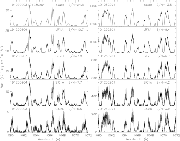
Figure 2. Coadded data compared to data from the individual channels. The top row of plots present regions of coadded spectra. The panels below this top row show data from individual channels that went into the coadds. The left panels show spectra observed in total eclipse, with the coadded spectrum at the upper left, and four representative detector channels contributing to this coadded spectrum shown in the panels below. (Eight individual channels were coadded for this region of the total eclipse spectrum.) The right panels show spectra from the ingress observation (D1230201), with the coadded spectrum at the upper right, and all four channels contributing to this observation shown below. The panels are selected in order of decreasing signal-to-noise ratio (S/N) from top to bottom. The S/N values shown are the 97th percentile S/N values of the entire channel. These S/N values are typical of peak fluxes of strong emission lines during eclipse and of the continuum out of eclipse. The individual channel data have been multiplied by the calibration factors given in Table 2. Spectra have been displaced vertically for clarity; zero levels for each spectrum are shown with horizontal lines.
Download figure:
Standard image High-resolution imageMany FUSE spectra show emission from airglow, with the strongest features due to H i, N i, N ii, and O i (Feldman et al. 2001). Scattered solar radiation can also appear in the SiC channels (Sonnentrucker et al. 2009), mostly notable in lines of C iii, O vi, and H i. These features can be distinguished from astronomical sources because the airglow and scattered solar radiation are stronger during orbital day than orbital night. Due to the brightness of 31 Cyg, and the resulting short exposure times, one would expect minimal contribution, and this is indeed the case. The portion of the 2003 July 18 total eclipse observation (D1230204) made during orbital day was compared to that made during orbital night (about half of this observation took place during orbital night and half during orbital day); the only significant differences were seen in the Lyman lines. The D1230203 observation was made mainly during orbital day, and minor differences between the two coadded D1230203 and D1230204 observations appear in the profiles of several O i lines, of N i 1134 Å, and possibly Ar i 1066 Å, probably attributable to airglow. C iii 977 Å shows substantial differences between these observations, possibly due to a variable solar scattered light contribution (see Figure 3 and further discussion of O i in Section 4). Airglow and scattered solar radiation should be even less significant in the out-of-eclipse spectra where flux from 31 Cyg is even greater and negligible for the small aperture HIRS observations.

Figure 3. Airglow/scattered solar radiation in the total eclipse spectra. The upper panel shows observations in the SiC2A channel in the total eclipse spectrum D1230204. The red line plots observations made entirely during orbital day, the green line plots observations made only during orbital night, and the black line plots their combination. No contribution from airglow is detected in the O i lines nor is scattered solar radiation observed in C iii. The lower panel compares fully coadded spectra. The D1230204 observation is plotted in black, and the D1230203 observation (which was mostly obtained during orbital day) is plotted in red. Major wavelength and intensity shifts are observed in the Lyman feature, but not in the O i lines. The C iii feature may have been affected by scattered solar radiation.
Download figure:
Standard image High-resolution imageBroad B-star absorption features are seen in the out-of-eclipse continuum. In order to best approximate the B-star contribution to the spectrum of 31 Cyg, FUSE archival spectra for B3-B5 IV-V stars were examined. The closest spectral match to the broad features in the phase 0.037 spectrum was HD 36981, a B5 V star near the Orion Nebula; see Murthy et al. (2005). The match is not good for the strength of the interstellar H2 spectrum, which is weaker in HD 36981 than in 31 Cyg. However, the HD 36981 spectrum provides a very good match for the broad underlying B-star features.
4. THE SPECTRUM DURING TOTAL ECLIPSE
The entire spectrum as seen during total eclipse is plotted in Figure 4. The total eclipse spectrum has been previously published by Bennett (2006), but that figure simply plotted all eight channels as extracted from the pipeline-processed MAST archive data set. In the preparation of our Figure 4, the combined, coadded eclipse spectrum of observations D1230203 and D1230204 is used. The complete, combined data set is presented in the total eclipse atlas. The strongest lines (truncated in this figure) are those of N ii UV multiplet 1. The second strongest lines (near 1130 Å) arise from Fe iii (UV 1). The strong lines seen near 990 Å are blends of N iii, Fe ii, and Si ii. The strong lines near 1150 Å are largely due to Fe ii. Other ions that produce emission features with peak fluxes ≳ 5 × 10⁻¹² erg cm−2 s−1 Å−1 are P ii, S ii, S iii, O i, and Ar i.

Figure 4. FUSE spectrum of 31 Cygni during total eclipse. The strong lines of N ii near 1085 Å have been truncated. Their profiles are shown in Figure 9.
Download figure:
Standard image High-resolution imageThe total eclipse atlas is plotted in Figure 5. Although the FUSE data extend down to 905 Å, no stellar emission features were visible shortward of 940 Å, so those data are not shown in the atlas plots.

Figure 5.
Sample page from the total eclipse atlas. The ordinate is wavelength in Å. Red lines mark features identified from the Hirata & Horaguchi (1995) database. These features are annotated with wavelength in Å, ion, lower and upper energy levels in eV, log gf, a "strength" quantity (described in the text), and multiplet designation (if available). Dotted lines mark lines which could be identified with transitions with gf-values weaker than other lines from the same ion that were not observed. Positions of interstellar features which cut into observed emission features, or which could affect the edges of emission line profiles, are marked with blue lines. O vi was not detected, but the wavelengths where these features would have been seen have been marked with green lines. The page starting with 1080 Å is plotted at two different scales to show the strong N ii (UV 1) lines as well as weaker features. (A color version, the complete figure set (26 images), and supplementary data for this figure are available in the online journal.)
Download figure:
Standard image High-resolution imageEmission lines were identified using the database of predicted atomic features compiled by Hirata & Horaguchi (1995). The database was sorted based on the upper energy levels of the transitions. For a given ion and a given upper level, the presence or absence of lines was noted as a function of log gf. The choice of the minimum log gf included for a given upper level involved a trade-off between having plausible identifications for as many features as possible, while minimizing the labeling of features that were not actually detected. Each identified feature is annotated with its rest wavelength, ion, upper and lower levels in eV, log gf, a "strength" quantity, and a multiplet designation, if available. The "strength" quantity is the difference between the minimum log gf used for inclusion of that upper level and the actual log gf for the line. This quantity is useful in estimating the degree of contribution to a blend from different ions. A colon after the strength quantity indicates that there were too few lines from a given ion for a well-defined minimum log gf to be determined. Table 3 lists the ions which were seen in the spectrum and the minimum log gf to which transitions were included as a function of upper level.
Table 3. Upper Level Ranges for Emission Lines Seen in Totality
| Ion | Lower | Upper | Minimum | Number |
|---|---|---|---|---|
| Cutoff (eV) | Cutoff (eV) | log gf | of Lines | |
| C ii | 0.0 | 13.00 | −1.0: | 2 |
| C iii | 0.0 | 13.00 | −1.0: | 1 |
| N i | 0.0 | 12.95 | −2.0 | 8 |
| N ii | 0.0 | 12.00 | −3.0: | 6 |
| N iii | 0.0 | 13.00 | −2.0: | 3 |
| O i | 0.0 | 12.00 | −2.5 | 3 |
| O i | 12.0 | 15.00 | −1.0 | 4 |
| Si ii | 0.0 | 13.00 | −2.0: | 5 |
| P ii | 0.0 | 13.00 | −2.0 | 20 |
| P iii | 0.0 | 13.00 | −1.0: | 2 |
| S ii | 0.0 | 15.00 | −1.5 | 14 |
| S iii | 0.0 | 13.00 | −2.0: | 7 |
| Cl ii | 0.0 | 12.00 | −1.9 | 6 |
| Cl iii | 0.0 | 13.00 | −1.6: | 3 |
| Ar i | 0.0 | 12.00 | −2.0: | 2 |
| Cr iii | 0.0 | 13.00 | −1.0 | 17 |
| Cr iii | 13.0 | 14.00 | −0.6 | 10 |
| Cr iii | 14.0 | 15.00 | 0.0 | 5 |
| Fe ii | 0.0 | 14.00 | −1.0 | 121 |
| Fe iii | 0.0 | 12.00 | −2.0 | 9 |
| Fe iii | 12.0 | 16.00 | −0.5 | 13 |
| Ni ii | 0.0 | 13.30 | −1.0 | 22 |
| Ni ii | 13.3 | 16.00 | −0.3 | 8 |
| Ge iii | 0.0 | 12.00 | 0.0: | 1 |
Download table as: ASCIITypeset image
Some features could be identified by lines of O i and Fe ii with log gf values somewhat less than the cutoff for that upper level. These features are annotated with dotted lines and negative values for the strength quantity. As discussed below, it is likely that these lines are excited by absorption of B-star photons.
Several lines of evidence (in addition to the agreement between orbital day and night observations discussed in Section 3) indicate that the O i emission seen in 31 Cyg is mostly stellar rather than due to airglow. First, the strong zero-volt lines show interstellar absorption at the same radial velocity as other interstellar lines. Second, the radial velocities of the O i lines are similar for the two eclipse observations, which is not the case for the Lyman airglow lines. Finally, the relative strengths between multiplets differs from that seen in airglow. For example, in the airglow spectrum, multiplet UV 4 is much stronger than multiplet UV 7 (Feldman et al. 2001), whereas multiplet UV 7 is clearly detected in 31 Cyg, while multiplet UV 4 is not. Emission from multiplets UV 3, 5, and 7 is detected in 31 Cyg, but not from multiplets UV 4 nor 10, despite similar f-values for the strongest lines. This behavior can be understood by recognizing that the multiplets which do not appear have wavelengths that lie within the strong B-star Lyman absorption, so their upper levels are not excited by the absorption of B-star flux. The absorption that excites the observed multiplets is clearly detected in the phase 0.989 and 0.014 observations.
It should be noted that while emission from the 1023.700 Å line of Si ii UV 5.01 is seen within the wavelength region of strong B-star Lyman absorption, its upper term could be excited by other lines in the same multiplet.
The Fe ii lines seen in emission despite lower gf-values for their upper energy levels all arise from the ground term, and all have strong enough chromospheric eclipse absorption to have broad, essentially black cores in the phase 0.989 observation. These lines continue to show very strong (albeit still with non-zero flux) absorption in the phase 0.014 observation. Thus, the upper levels in these transitions can be excited from the absorption of B-star flux.
Many of the emission features are cut by interstellar absorption, either by H2 or (for zero-volt lines) from the same transition. This absorption is labeled with solid blue lines. Considerably more H2 absorption features were detected outside total eclipse, but not all are labeled in the total eclipse atlas in order to avoid unnecessary clutter; the only H2 absorption features marked here are those that might affect the profiles of observed emission lines. In addition to H2, interstellar absorption is detected in C ii, C iii, N i, N ii, N iii, O i, Si ii, P ii, Ar i, and Fe ii.
Representative line profiles for the zero-volt emission features that are cut by interstellar absorption are shown in Figure 6. For the lines plotted in the left panel, the short-wavelength peak is stronger, while the long-wavelength peak is stronger for lines plotted in the right panel. In general, lower states of ionization tend to show profiles in which the short wavelength emission peak is stronger. Profiles for representative emission features not affected by interstellar absorption are shown in Figure 7, and these profiles explain the differences observed in the features cut by interstellar absorption. Note the difference in shape between the Fe ii and Fe iii features. Emission features of Fe ii are fairly symmetric and centered near or slightly shortward of line center, relative to the −7.7 km s−1 systemic velocity of Wright (1970), while the Fe iii features are asymmetric and redshifted. These profiles are consistent with emission line profiles seen in IUE spectra of 31 Cyg during total eclipse, in which most singly ionized lines showed profiles centered near rest wavelength, while lines from doubly and triply ionized species showed red-shifted and sometimes asymmetric profiles (Bauer & Stencel 1989). Stencel & Chapman (1981) had observed similar profiles in ζ Aur, which they interpreted as resulting from flow in a bow shock around the hot companion.
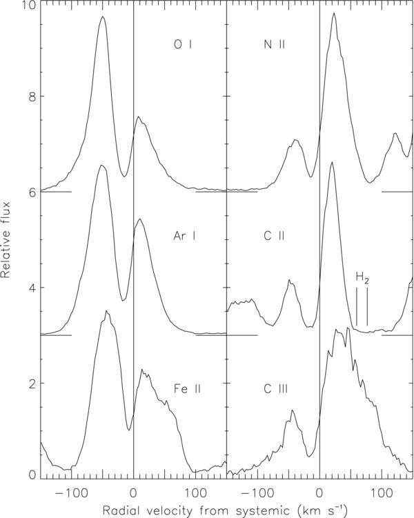
Figure 6. Representative emission line profiles cut by interstellar absorption. Individual lines included are: O i 1039.230 Å, Ar i 1048.220 Å, Fe ii 1144.938 Å, N ii 1083.994 Å, C ii 1036.337 Å, and C iii 977.020 Å. Note that the long-wavelength edge of the C ii profile is affected by interstellar H2.
Download figure:
Standard image High-resolution image
Figure 7. Representative emission line profiles not cut by interstellar absorption. Individual lines included are O i 1040.943 Å, Fe ii 1068.346 Å, Fe iii 1122.533 Å, Si ii 1023.700 Å, P ii 1153.995 Å, and P iii 1003.600 Å.
Download figure:
Standard image High-resolution imageAnother possibility is that the emission profiles simply reflect the distinct regions in which they are formed. The extended chromosphere near the K supergiant is mostly neutral in H i, but metals are mostly singly ionized. In contrast, the stellar wind, with a terminal velocity of ∼80 km s−1, must be mostly ionized (Eaton 2008) in order to account for the large 6 cm radio continuum flux observed by Drake et al. (1987). In an H ii region, it is expected that most metals will be doubly ionized, e.g., Fe will be present mainly as Fe iii. Therefore, the low-ionization lines, such as Fe ii, should be formed in a mainly static extended spherical region around the K supergiant (with a possible extension in the direction of the K star's shadow away from the B star). The result: these lines should show broad velocity peaks near the K star velocity as observed. (The radial velocities of both stars near eclipse are close to systemic as their movement is nearly transverse to the line of sight). The high-ionization lines are formed in the outflowing stellar wind, and thus their formation region is dominated by photons scattered close to the B star ultraviolet source. Near eclipse, the B star is "behind" the K star as seen from Earth, and emission (or scattering) from the wind near the B star is therefore redshifted. This schematic model accounts for the observed velocity profile of lines such as Fe iii. Detailed radiative transfer calculations will be required to verify this line formation model.
The resonance lines of O vi have been detected with FUSE in many astrophysical sources, including accretion disks and cool star chromospheres, but were not detected in 31 Cyg. Their wavelengths have been marked with green lines to show the non-detection. As previously described, there was no evidence for time-varying variation (that would presumably result from accretion) seen in the emission line profiles between the 2003 June 30 and July 18 observations, except in the C iii 977 Å line, which could result from accretion and/or scattered solar radiation.
Several relatively strong features remain unidentified. Those with peak fluxes ≳ 2.5 × 10⁻¹³ erg cm−2 s−1 Å−1 above any faint continuum are listed in Table 4.
Table 4. Unidentified Emission Features
| Wavelength | Peak Fluxa | Wavelength | Peak Fluxa |
|---|---|---|---|
| (Å) | (Å) | ||
| 1016.7 | 3.6 | 1163.7 | 4.0 |
| 1053.4b | 3.3 | 1167.5 | 2.9 |
| 1057.2c | 4.3 | 1174.0 | 4.3 |
| 1058.9 | 2.7 | 1186.1 | 7.6 |
| 1095.7d | 3.3 | 1186.9 | 7.8 |
| 1158.1d | 3.5 |
Notes. a10−13 erg cm−2 s−1 Å−1 above background. bShort-wavelength edge cut by H2. cLong-wavelength edge cut by H2. dBlended with a stronger feature.
Download table as: ASCIITypeset image
An emission feature near 1008.5 Å shows an asymmetric profile consistent with the redshifted lines from high-ionization species like Fe iii. Its wavelength matches that of the resonance line of Ge iii. It is not out of the question that germanium could be detected. Its abundance in the Sun is not very different from that of vanadium, 3.65 in the log, as opposed to 3.93 for vanadium, with H = 12 (Asplund et al. 2009). V ii absorption was clearly seen in 31 Cyg in IUE spectra taken during chromospheric eclipse. Since vanadium and germanium have similar ionization potentials, one might expect to see V iii in the total eclipse spectrum. Most of the V iii lines fell in crowded regions of the spectrum, but the 1125.699 Å line of multiplet 3, with a log gf of −0.11, lies in a relatively clear region and was not seen. The Ge iii line has a log gf of +0.25. If these elements were present in their solar abundances, one would have expected to see the V iii line at approximately the same strength as the Ge iii line. Thus, if this feature is indeed due to Ge iii, germanium must be overabundant relative to vanadium. This Ge iii line has been detected in several planetary nebulae (Sterling et al. 2002). The authors concluded that Ge needed to be overabundant to be detected and noted a possible explanation in that most of the nebulae with detected Ge had Wolf–Rayet central stars, whose winds could expose processed material. Such an explanation makes less sense for 31 Cyg; however, due to the excellent wavelength and profile shape agreement, as well as the lack of any other plausible identification, we tentatively ascribe this feature to Ge iii.
5. THE SPECTRUM DURING CHROMOSPHERIC ECLIPSE
Outside of total eclipse, a chromospheric absorption spectrum is visible, which decreases in strength as the stars move farther apart. By orbital phase 0.037, only a few weak chromospheric absorption features remain, leaving a spectrum dominated by broad B-star features and narrow interstellar H2. We show the combined coadded spectrum of observations D1230206 and D1230207 at phase 0.037 in the chromospheric eclipse atlas.
The chromospheric eclipse atlas is shown in Figure 8. Chromospheric absorption lines are marked with blue lines and labeled as in Figure 5, and interstellar H2 absorption features are marked with red lines. The observed wavelengths of weak chromospheric features in the phase 0.989 spectrum were measured, and the average agreed to the radial velocity of the H2 lines to within 1 km s−1. Therefore, the chromospheric lines were marked at a radial velocity of −16 km s−1 to better match their positions in the phase 0.989 observation. Despite the radial velocity agreement between the H2 features and weak chromospheric features, the H2 is indeed interstellar and not chromospheric as can be seen by noting that the H2 absorption features do not decrease in strength as the stars move away from eclipse, whereas the chromospheric absorption does.
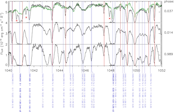
Figure 8.
Section of the chromospheric eclipse atlas. The ordinate is wavelength in Å. All three spectra of 31 Cyg (black lines) are plotted to the same scale. The green line in the upper panel is the spectrum of HD 36981 (B5 V), scaled in wavelength and flux to best represent the contribution of the B star in the 31 Cyg spectra. The total eclipse spectrum of 31 Cyg is plotted in gray and filled in; where the emission is weak, the gray line provides a zero point for the two upper panels. Vertical red lines mark absorption features due to H2. Vertical blue lines mark the absorption transitions selected from the Hirata & Horaguchi (1995) database and are annotated with wavelength, ion, lower and upper energy levels in eV, log gf, a "strength" quantity (described in the text), and multiplet designation (if available). Red asterisks mark wind absorption features seen ∼80 km s−1 shortward of a few strong features. (The complete figure set (24 images) and supplementary data for this figure are available in the online journal.)
Download figure:
Standard image High-resolution imageLine identifications for the chromospheric absorption spectrum were again made from the Hirata & Horaguchi (1995) database. The same procedure was used, but by using the lines' lower energy levels. The ions which give rise to observable features, along with the cutoffs in log gf, are listed in Table 5. In some cases (although not on the sample page plotted here), several transitions of significantly differing strengths might be contributing to a blend. Labeling of some of the weaker transitions close in wavelength to significantly stronger ones is suppressed to avoid confusion, and these weaker features are marked with dotted gray lines. Especially strong features are labeled with darker blue lines and bolder font. The full list of selected transitions including term designations is given in Table 6.
Table 5. Lower Level Ranges for Absorption Lines Seen During Chromospheric Eclipse
| Ion | Lower Level | Upper Level | Minimum | Number |
|---|---|---|---|---|
| Cutoff (eV) | Cutoff (eV) | log gf | of Lines | |
| N i | 0.00 | 1.00 | −6.0: | 24 |
| N ii | 0.00 | 4.00 | −6.0: | 8 |
| O i | 0.00 | 2.00 | −4.0: | 40 |
| Si ii | 0.00 | 0.10 | −2.0: | 5 |
| P ii | 0.00 | 1.00 | −2.5 | 19 |
| P ii | 1.00 | 2.00 | −1.0 | 3 |
| S ii | 1.00 | 2.00 | −2.0 | 8 |
| S ii | 2.00 | 3.50 | −1.2 | 6 |
| Cl i | 0.00 | 10.00 | −1.0 | 17 |
| Ar i | 0.00 | 10.00 | −6.0: | 2 |
| Cr ii | 0.00 | 1.00 | −2.6 | 13 |
| Mn ii | 0.00 | 1.00 | −2.0: | 3 |
| Fe ii | 0.00 | 0.20 | −3.0 | 129 |
| Fe ii | 0.20 | 0.50 | −2.6 | 132 |
| Fe ii | 0.50 | 1.50 | −2.5 | 121 |
| Fe ii | 1.50 | 3.00 | −1.0 | 52 |
| Ni ii | 0.00 | 1.00 | −3.0 | 4 |
| Ni ii | 1.00 | 3.00 | −1.2 | 61 |
Download table as: ASCIITypeset image
Table 6. All Absorption Lines Selected from the Hirata & Horaguchi (1995) Database
| Wavelength | Ion | Lower | Upper | log | Relative | Multiplet | Lower | Upper |
|---|---|---|---|---|---|---|---|---|
| (Å) | Level | Level | gf | Strengtha | Term | Term | ||
| (eV) | (eV) | |||||||
| 950.112 | O i | 0.02 | 13.07 | −1.84 | 2.16: | U12 | 2p4 3P | 5d 3D* |
| 950.112 | O i | 0.02 | 13.07 | −2.32 | 1.68: | U12 | 2p4 3P | 5d 3D* |
| 950.510 | Cr ii | 0.00 | 13.04 | −0.94 | 1.66 | a6S | p4D* | |
| 950.594 | Cr ii | 0.00 | 13.04 | −1.13 | 1.47 | a6S | 5D 4f6H* | |
| 950.733 | O i | 0.03 | 13.07 | −2.19 | 1.81: | U12 | 2p4 3P | 5d 3D* |
| 950.810 | Cr ii | 0.00 | 13.04 | −0.48 | 2.12 | a6S | d4 4f6P* | |
| 950.885 | O i | 0.00 | 13.04 | −2.10 | 1.89: | U11 | 2p4 3P | 6s 3S* |
Only a portion of this table is shown here to demonstrate its form and content. A machine-readable version of the full table is available.
Download table as: DataTypeset image
A similar process was used to select H2 absorption features for labeling in the atlas. H2 Lyman band data from Abgrall et al. (2000), Werner band data from Abgrall et al. (1993a), and radiative dissociation data from Abgrall et al. (1993b) were used to produce a list of H2 features which could be present in typical interstellar conditions. These lists were used to identify features in the 31 Cyg spectra. Transitions with excitation potential up to 0.02 eV were included down to log gf = −3, transitions with excitation potential between 0.02 and 0.15 eV were included down to log gf = −2, and transitions between 0.15 and 0.25 eV were included down to log gf = −1.
Although the FUSE data extend down to 905 Å, too little flux was observed shortward of 950 Å to warrant including this region in the plotted atlas. Although some continuum is seen from ∼935 to 943 Å between two Lyman lines, the only spectral features seen there arise from interstellar H2.
All three spectra of 31 Cyg are plotted at the same scale but displaced vertically for clarity. The total eclipse spectrum is plotted at the same scale, as filled-in gray. These gray emission profiles produce an effective zero point for much of the spectra in the upper two panels. It also shows that some of the strong chromospheric absorption lines are bottoming out on the emission seen during totality, as was observed in the M + B eclipsing binary VV Cep (Bauer et al. 2007). In the sample page plotted here, this can be seen for the 1048.2 Å line of Ar i at phases 0.989 and 0.014. Even at phase 0.037, the N ii chromospheric absorption is deep enough to bottom out on the emission, as shown in Figure 9. Underlying Fe iii emission is observed to control the shape of Fe ii chromospheric absorption in several lines in the 1120–1130 Å region of the spectrum in the phase 0.989 and 0.014 observations. This behavior, the "bottoming out" of chromospheric absorption on the eclipse emission lines, confirms that these eclipse lines are formed in an extended region independent of the absorption component seen in chromospheric eclipse.
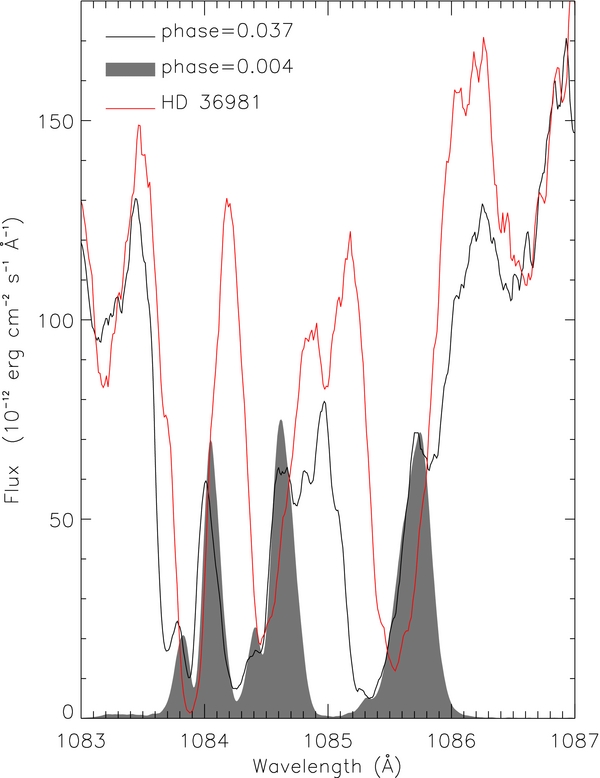
Figure 9. N ii (UV 1) lines. The filled gray represents emission features seen during total eclipse. The black line represents the FUSE spectrum obtained farthest from eclipse, and absorption in these features is still strong enough to bottom out on the emission seen during totality. The dip in the zero-volt 1084.0 Å emission line is due to interstellar N ii, while the dip in the 0.01 eV 1084.6 Å emission line is due to interstellar H2. The red line plots the FUSE spectrum of HD 36981 (B5 V), representing the expected contribution from the B star. The additional absorption in the N ii lines in the 31 Cyg spectrum is blue-shifted and is likely due to the K-star wind. Fluxes for HD 36981 have been multiplied by a factor of 3.5 and plotted with a blue shift of 55 km s−1 to align the B-star features. All data have been smoothed using a boxcar average with a 5-pixel width (one pixel is 0.01 Å).
Download figure:
Standard image High-resolution imageMany strong chromospheric lines appear doubled in the phase 0.014 spectrum, although none of these lines are seen in the sample page printed here. Several of these line profiles are plotted in Figure 10. This sort of line doubling is often seen in ζ Aur binaries during chromospheric eclipse. The line doubling in this observation is not caused by line profiles bottoming out on emission seen during total eclipse.

Figure 10. Doubled chromospheric absorption features seen at phase 0.014. The spectra at radial velocity +20 km s−1 are in the same top-to-bottom order as the line identification labels.
Download figure:
Standard image High-resolution imageThe green line in the upper panel of Figure 8 is the archival FUSE spectrum for the B5 V star HD 36981, scaled in both flux and wavelength to best match the broad B-star features in the 31 Cyg spectrum. While the interstellar H2 absorption is much weaker in HD 36981, the broad B-star absorption lines provide a good match to the B4 component in 31 Cygni. In the atlas page printed here, one can see that the 31 Cyg spectrum at phase 0.37 still shows chromospheric absorption due to O i and Ar i. Some features of Fe ii still show chromospheric absorption at this epoch, as shown in Figure 11.
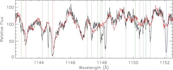
Figure 11. Chromospheric and wind lines seen at phase 0.037. The farthest from eclipse FUSE spectrum of 31 Cyg (phase 0.037, black line) is compared to B-star analog HD 36981 (red line), which has been scaled in wavelength and flux to align the B-star features. Vertical gray lines mark chromospheric absorption from excited Fe ii, red lines mark zero-volt Fe ii lines, and the blue line marks a 1.97 eV line of O i. Wind features are marked with green lines plotted 75 km s−1 shortward of many of the chromospheric features.
Download figure:
Standard image High-resolution imageA few strong transitions show sharp absorption features displaced by about −80 km s−1 from chromospheric lines in the phase 0.037 spectrum. These features are attributed to the expanding wind of the K supergiant and are labeled with red asterisks. These wind lines are seen in strong lines of O i, Ar i, and Fe ii. (See Figure 11.) These features are consistent with line profiles observed in the higher-resolution HST spectra. The HST spectra were obtained well outside chromospheric eclipse, and in addition to the interstellar absorption from zero-volt lines, blueshifted absorption from the K star wind was detected in C ii, O i, Mg ii, Al ii, Si ii, S ii, and Fe ii, as well as in Al iii and Fe iii. The strongest lines have essentially zero flux in their profiles between the interstellar absorption component at −16 km s−1 and the blueshifted wind absorption feature near −80 km s−1. Weaker lines show multiple wind absorption components.
Some strong chromospheric absorption lines were not identified by our procedure; in the atlas page plotted here, strong unidentified features are seen near 1043 and 1044 Å. A list of unidentified features with equivalent width ≳80 mÅ in the phase 0.989 spectrum is presented in Table 7.
Table 7. Unidentified Absorption Features in Deep Chromospheric Eclipse
| Wavelength | EQW | Wavelength | EQW |
|---|---|---|---|
| (Å) | (mÅ) | (Å) | (mÅ) |
| 956.3 | 120 | 1057.2a | 200 |
| 961.5a | 360 | 1076.6a | 610 |
| 963.0a | 370 | 1098.6a | 180 |
| 1000.2a | 350 | 1130.9a | 110 |
| 1001.3 | 140 | 1139.8a | 110 |
| 1005.0a | 90 | 1141.1 | 150 |
| 1006.1a | 160 | 1143.7a | 330 |
| 1034.4a | 150 | 1155.9a | 100 |
| 1043.1 | 360 | 1164.0a | 330 |
| 1044.0 | 210 | 1167.5 | 430 |
| 1044.6a | 210 | 1169.7a | 160 |
| 1052.1a | 400 | 1176.5a | 480 |
| 1053.2a | 480 | 1177.7 | 340 |
| 1054.2a | 270 |
Note. aBlended: wavelength and EQW may be affected.
Download table as: ASCIITypeset image
There are relatively few differences between the phase 0.037 spectrum of 31 Cygni and the B-star proxy HD 36981. Chromospheric and wind absorption in O i and Ar i were shown in Figure 8, and blended absorption from the chromosphere and wind in N ii were shown in Figure 9. Chromospheric and wind absorption is also seen in Fe ii, as shown in Figure 11; sharp absorption features are observed for excited lines of Fe ii in the 31 Cyg spectrum, while only the interstellar lines expected from zero-volt Fe ii are seen in HD 36981.
6. OTHER ZETA Aur BINARIES
These atlases will be useful for working with far-UV spectra of other ζ Aur binaries. Figure 12 compares a section of the best-exposed chromospheric eclipse spectrum of 31 Cyg to archival FUSE spectra of KQ Pup (M2Iab + B0Ve), 32 Cyg (K4-5 Ib + B6-7 IV-V), and VV Cep (M2Iab + B?). Many of the same features are seen in both objects. Gray vertical lines denote Fe ii absorption. Many of these lines were doubled in this observation of 31 Cyg, and the line annotations have been centered on the shorter-wavelength component. The other three spectra have been scaled in flux to show approximately the same contrast as the 31 Cyg spectrum and shifted in wavelength so that their absorption features line up with those of 31 Cyg. It is clear that chromospheric absorption features from Fe ii are present in all four objects. Green lines mark the shortward component of doubled P ii absorption features in 31 Cyg. While P ii absorption is visible in all four objects, it is considerably weaker in 32 Cyg than in the others. The two P ii features at ∼1155 and 1157 Å are not blended with known features. Note how the doubling in the 1157 Å feature is seen in all four objects. The blue line marks a 1.97 eV O i line. The profile of this feature shows more variation between the objects than do the other lines in this region of the spectrum and could have been affected by airglow. The unidentified feature(s) near 1156 Å is present in 31 Cyg, VV Cep, and KQ Pup, but not in 32 Cyg.

Figure 12. Chromospheric eclipse in 31 Cyg (at phase 0.014) compared to the archival FUSE spectra of other ζ Aur binaries. The spectra of VV Cep, 32 Cyg, and KQ Pup have been scaled and displaced in flux for clarity and shifted in wavelength to align similar features. Gray lines mark features due to Fe ii, green lines P ii, and the blue line O i. Zero-point fluxes are marked with horizontal lines at the left of the figure, color-coded to match the plotted spectra.
Download figure:
Standard image High-resolution image
7. SUMMARY
We present an atlas of coadded FUSE spectra of the ζ Aur binary system 31 Cyg during total eclipse, two epochs of chromospheric eclipse (phase 0.989 and 0.014), and one epoch near the end of chromospheric eclipse (phase 0.037). We include all available FUSE detector channels in this reduction and describe the details of the calibration and coaddition process. The resulting spectra are available in the online version of the journal. Interstellar absorption from H2 is seen in all observations, and interstellar absorption from strong zero-volt atomic species is seen in total eclipse and in the phase 0.037 egress observation. During the other chromospheric eclipse observations, interstellar features from atomic lines are blended with chromospheric absorption.
A rich emission spectrum is observed during total eclipse. These emission features appear to form in two distinct regions. Relatively low ionization states (e.g., Fe ii and O i) show profiles centered close to the systemic velocity, or somewhat blueshifted, and appear to be excited from absorption of B-star flux in the chromosphere/inner wind of the K supergiant. Lines of higher ionization state (e.g., Fe iii and Cr iii) show asymmetric, redshifted profiles. These high ionization states are not detected in absorption during chromospheric eclipse.
During chromospheric eclipse, absorption features from neutral and singly ionized elements are seen, the large majority of which arise from Fe ii. Many of the strongest features appear doubled in the phase 0.014 observation. In deep chromospheric eclipse, the profiles of some of the strongest lines are controlled by bottoming out on the emission seen during total eclipse. In the phase 0.037 observation, some weak chromospheric absorption remains from strong lines of low-excitation Fe ii, O i, and Ar i, and absorption blueshifted by ∼80 km s−1 is seen from the wind of the K supergiant. While most of the features have plausible identifications, numerous strong features do not.
These atlases should be useful in work with the far-UV spectra of other ζ Aur systems as the chromospheric eclipse spectra look quite similar to those of 32 Cyg, KQ Pup, and VV Cep. The coadded data sets produced will provide a basis for future analyses of the fundamental stellar parameters and atmosphere of the 31 Cyg K supergiant star.
We are grateful to B. Wood for providing us with an IDL script to predict interstellar H2 features. P.D.B. was supported by NASA grant NAG5-13705 to the University of Colorado. W.H.B. acknowledges support from Wellesley College. This research has made use of the SIMBAD database, operated at CDS, Strasbourg, France.