


ABSTRACT
Presented are the results of a near-IR photometric survey of 1678 stars in the direction of the ρ Ophiuchus (ρ Oph) star forming region using data from the 2MASS Calibration Database. For each target in this sample, up to 1584 individual J-, H-, and Ks-band photometric measurements with a cadence of ∼1 day are obtained over three observing seasons spanning ∼2.5 yr; it is the most intensive survey of stars in this region to date. This survey identifies 101 variable stars with ΔKs-band amplitudes from 0.044 to 2.31 mag and Δ(J − Ks) color amplitudes ranging from 0.053 to 1.47 mag. Of the 72 young ρ Oph star cluster members included in this survey, 79% are variable; in addition, 22 variable stars are identified as candidate members. Based on the temporal behavior of the Ks time-series, the variability is distinguished as either periodic, long time-scale or irregular. This temporal behavior coupled with the behavior of stellar colors is used to assign a dominant variability mechanism. A new period-searching algorithm finds periodic signals in 32 variable stars with periods between 0.49 to 92 days. The chief mechanism driving the periodic variability for 18 stars is rotational modulation of cool starspots while 3 periodically vary due to accretion-induced hot spots. The time-series for six variable stars contains discrete periodic "eclipse-like" features with periods ranging from 3 to 8 days. These features may be asymmetries in the circumstellar disk, potentially sustained or driven by a proto-planet at or near the co-rotation radius. Aperiodic, long time-scale variations in stellar flux are identified in the time-series for 31 variable stars with time-scales ranging from 64 to 790 days. The chief mechanism driving long time-scale variability is variable extinction or mass accretion rates. The majority of the variable stars (40) exhibit sporadic, aperiodic variability over no discernable time-scale. No chief variability mechanism could be identified for these variable stars.
1. INTRODUCTION
Photometric variability in young stars is an ubiquitous phenomenon. Physical mechanisms causing this variability include, but are not limited to, the rotational modulation of starspots, evolution of the circumstellar environment, interstellar extinction, transit events and stellar pulsation. Large sample variability studies, such as by Herbst et al. (1994), indicate that these mechanisms often operate concurrently resulting in very complex photometric time-series in T Tauri stars. Interpretations are primarily limited because broad band photometry acquired by seeing-limited telescopes are unable to spatially resolve the inner regions around young stars, which are on the order of milliarcseconds for low mass stars in nearby star-forming regions.
High cadence, long temporal baseline photometric surveys, however, can temporally resolve the variations and help identify the dominant mechanism responsible for the variability. This type of survey work has the prospect of identifying peculiar observational phenomenon that may hold clues to unsolved problems in star and planet formation. One example is the physical interpretation for AA Tau-like variability (Bouvier et al. 2003). This variability presents as discrete drops in flux from a nearly constant "continuum" flux level. The phenomenon is not unique to this star; Morales-Calderón et al. (2011) identified 38 stars exhibiting similar variability during an intensive photometric monitoring campaign of young stellar objects (YSOs) in the Orion Nebula Cluster. They found that these dips have durations of 1 to a few days decreasing the flux by several tenths of magnitude in the IRAC bands and as much as 1.5 mag in the J band. These dips either appeared only once in 40 days (the survey's temporal baseline) or appeared periodically every 2 to 14 days. The current physical interpretation for these observations is periodic obscuration of the star by a high latitude "warp" in the circumstellar disk (Bertout 2000; Bouvier et al. 2003). Longer temporal baseline photometric monitoring of additional YSOs will place better constraints on the periodic nature of these events, which in turn will confirm/constrain the current physical interpretation.
Intensive photometric monitoring is most useful when it is conducted at a range of wavelengths. Near-IR observations probe the very inner regions from ∼0.01 to 1 AU for low mass stars (Dullemond & Monnier 2010). As young stars are typically rapidly rotating, this region includes both the co-rotation radius and dust sublimation radius. For a median disk lifetime of 5 Myr, this corresponds to millions of dynamical times at these orbital radii (Haisch et al. 2001). Therefore any indication of asymmetries in the circumstellar disk must be driven by some phenomenon (i.e., inclined magnetic dipole, planetary formation). Understanding the physics in this region is of particular interest to protoplanetary formation and migration, as well as how mass accretes onto the star.
ρ Ophiuchus (ρ Oph) makes an excellent laboratory to test the ability of high cadence, long temporal, near-IR observations to distinguish between variability mechanisms in young stars. ρ Oph is a dense star-forming region containing a few hundred known young stellar objects (YSOs) with ages ranging from 0.3 to 3 Myr. The region is rich with variable stars; previous surveys have identified more than 100 photometrically variable stars (Greene & Young 1992; Barsony et al. 1997, 2005; Bontemps et al. 2001; Wilking et al. 2005; Alves de Oliveira & Casali 2008). Photometric surveys are limited to the near- to far-IR due to large amounts of visual extinction ranging from 5 to 25 AV in the cloud core (Cambrésy 1999). This complex interstellar environment could itself be responsible for detected photometric variability.
Plavchan et al. (2008, hereafter P08) carried out a pilot study of 57 stars in the ρ Oph field using photometry collected by the Two Micron All Sky Survey Calibration Point Source Working Database (2MASS Cal-PSWDB). That study identified periodic variability in two YSOs given a sample of candidate M stars. The study presented here expands on the initial pilot study performed in P08 and will include the full ρ Oph field data set from the 2MASS Cal-PSWDB to better understand the variability of young stars in this cloud.
In Section 2, the details concerning the observations and source selection for this survey are discussed. The variability analysis, along with a discussion on advantages to high cadence observations, is presented in Section 3. The methods used to find both periodic and long time-scale variability are found in Section 4. In Section 5, the characteristics of the variability catalog, as well as a discussion of variability mechanisms is presented. That section also discusses six stars where two variability mechanisms are estimated to operate concurrently. Finally Section 6 contains a summary of the findings reported by this work.
2. OBSERVATIONS AND SAMPLE SELECTION
2.1. Observations
The Two Micron All-Sky Survey (2MASS, Skrutskie et al. 2006) imaged nearly the entire sky via simultaneous drift scanning in three near-infrared bands (JHKs) between 1997 and 2001. Observations were taken at the northern Mt. Hopkins Observatory and the southern CTIO facility. Photometric calibration for 2MASS required hourly observations of 35 calibration fields split evenly between the northern and southern hemispheres. Each calibration field is 1° in length and 8 5 wide. One calibration field lies in the direction of the Ophiuchus constellation. This field is centered at α = 16h27m15
 6 and δ = −24°41'23'' (J2000) and covers part of the ρ Oph L1688 cloud core (Bok 1956). These data have an observation cadence of ∼1 epoch per day. A complete observation is comprised of six consecutive 1.3 s scans in declination with a nearly constant right ascension. Each scan is offset by 5'' in right ascension to minimize errors from pixel effects. The six scans, or "scan group," are finally co-added to minimize short time-scale and systematic variations. A complete scan group is obtained in approximately 8 minutes (Cutri et al. 2003, Section III.2b). The maximum number of scans for a single star is 1584 divided by 6 or 264 scan groups.
Photometry is extracted from the calibration field via the 2MASS Point Source Catalog (2MASS PSC) automated processing system. Details of the system's implementation are described in Cutri et al. (2003); here a brief summary is given. Photometry for sources fainter than J = 9, H = 8.5, and Ks = 8 mag are extracted by profile-fitting. Profile-fitting compares the source flux to a pre-generated point-spread function (PSF) via χ2 minimization. The PSFs are selected from a look-up table with respect to a dimensionless seeing index that is updated regularly during each scan. The seeing index characterizes the atmospheric seeing during specific observations. The library of PSFs is generated by empirically fitting the 50 brightest stars in a single 2MASS calibration scan with a specific average seeing index. This scan is not necessarily of the ρ Oph field, but a calibration field containing a different slice of the sky. An error at the few-percent level may be present in the resulting photometry due to mismatched PSFs arising from rapid seeing variations.
For the few sources brighter than the above magnitude limits, photometry are extracted using a 4'' fixed aperture corrected using a curve-of-growth. Atmospheric seeing conditions can place as much as 15% of the flux from a point source outside this fixed aperture. A curve-of-growth correction is a constant factor added to measured photometry to simulate measurements taken using an "infinite" aperture. The benefit of this method is avoiding decreased signal-to-noise and potential source confusion arising from large aperture photometry. However, curve-of-growth corrections assume the sources are unresolved single stars that can be approximated by a PSF. Therefore photometry for extended sources (i.e., stars embedded in bright nebular emission) or multiple systems are not properly characterized with this method. All the data scans are compiled in the 2MASS Cal-PSWDB.
2.2. Source Identification
The source selection in the ρ Oph field is similar to that described in P08, which is summarized here. A parent sample catalog of 7815 sources is constructed from a co-added deep image of the field (Cutri et al. 2003). For each target in the parent sample, the 2MASS Cal-PSWDB is searched for detections within a 2'' matching radius. This radius is several σ larger than the 2MASS PSC astrometric precision and astrometric bias between the PSWDB and PSC (Zacharias et al. 2005; Skrutskie et al. 2006). This ensures confidence that all Cal-PSWDB detections for the parent 7815 sources are found within the PSC astrometric precision.
Of the 7815 stars identified in the parent sample, 1678 stars have a sufficient number of detections for variability and periodic analysis. This sample of 1678 stars is henceforth referred to as the target sample. A "sufficient number" is defined as stars detected in ⩾10% of the observations in either J, H or Ks and ⩾50 detections in the J band. The first constraint ensures a sufficient number of data points for a robust periodogram computation. The 10% limit is an ad hoc limit chosen to reduce the noise present in the variability statistics. The second constraint removes sources near the field of view edges that are not present in most scans.
Finally, despite the success of the 2MASS prescription to produce high-quality photometric measurements, occasionally photometry affected by latent image artifacts, spurious detections, and poor quality detections still persist in the database. The reader is referred to P08 for a full treatment on how sources with poor photometry are characterized and excluded. Cutri et al. (2003) describes the different varieties of latent image artifacts arising from a number of phenomenon associated with the optical system. These artifacts are identified and removed via visual inspection. Multiple simultaneous detections found within the 2'' search radius of a target, which are typically spurious byproducts of the source extraction pipeline, are eliminated. Simultaneous detections are when two (or more) detected sources are identified with a single source in the 2MASS Cal-PSWDB. Secondary detections are typically ∼0.5–1.5 mag fainter than the primary detection. In addition, they are typically detected in only one passband and only in one of the six scans. Unaccounted for spurious detections can give the appearance of variability and introduce systematic noise into any underlying periodic signals. Photometric measurements with poor spatial fits to the model PSF are also excluded from our analysis. A poor spatial fit occurs when the χ2 value between the observed stellar profile and a model PSF is >10. This is flagged as "E" quality photometry within the Cal-PSWDB. Image saturation, cosmic rays, hot pixels, extended emission, or partially resolved doubles could account for this poor quality fit to the photometry (Cutri et al. 2003). Photometry with poor spatial fits are systematically brighter by a few tenths of a magnitude, and this can falsely trigger the identification of variability.
Table 1, available only on-line, lists the 1678 stars analyzed for variability. The magnitudes and errors listed are extracted from a co-added image of all calibration scans in that particular band.
Table 1. Catalog of 2MASS Stars in ρ Oph
| R.A. | Decl. | NJobs | NHobs | NKobs | Ja | Ha | Ksa |
|---|---|---|---|---|---|---|---|
| (degrees) | (degrees) | (mag) | (mag) | (mag) | |||
| 246.730759 | −25.067987 | 262 | 261 | 244 | 16.972 ± 0.011 | 16.174 ± 0.012 | 15.659 ± 0.028 |
| 246.731262 | −25.062096 | 258 | 258 | 258 | 17.048 ± 0.016 | 16.163 ± 0.014 | 15.631 ± 0.029 |
| 246.731293 | −24.955822 | 6 | 70 | 72 | 16.508 ± 0.005 | 15.796 ± 0.006 | 15.431 ± 0.009 |
| 246.731308 | −25.015520 | 263 | 263 | 262 | 13.980 ± 0.001 | 13.048 ± 0.001 | 12.747 ± 0.001 |
| 246.731323 | −24.472427 | 6 | 41 | 32 | 17.272 ± 0.000 | 16.440 ± 0.043 | 15.327 ± 0.014 |
| 246.731323 | −25.130241 | 198 | 174 | 67 | 16.973 ± 0.010 | 16.211 ± 0.012 | 15.720 ± 0.026 |
| 246.731750 | −25.146633 | 187 | 139 | 47 | 16.987 ± 0.010 | 16.227 ± 0.013 | 15.726 ± 0.028 |
| 246.731796 | −24.863796 | 102 | 105 | 36 | 15.868 ± 0.003 | 15.030 ± 0.003 | 14.694 ± 0.004 |
| 246.731934 | −25.135702 | 16 | 4 | 11 | 16.107 ± 0.014 | 15.431 ± 0.017 | 15.150 ± 0.013 |
| 246.732269 | −25.137508 | 262 | 260 | 246 | 12.371 ± 0.001 | 11.786 ± 0.001 | 11.552 ± 0.001 |
Notes. aUnweighted mean apparent magnitude of Cal-PSWDB photometry.
Only a portion of this table is shown here to demonstrate its form and content. A machine-readable version of the full table is available.
Download table as: DataTypeset image
2.2.1. Detection and Completeness Limits
For non-variable stars, the photometric measurement uncertainty is characterized by the standard deviation of all photometric measurements in a particular band. P08 showed that this photometric standard deviation as a function of apparent magnitude, for 2MASS photometry, follows the form of two distinct power laws. One power law describes brighter sources, where Poisson statistics dominate the uncertainty, while the second describes the dimmer sources, where the uncertainty is dominated by instrumental noise. The point of intersection between these two power laws, or "break point," designates the survey completeness limit where source detection drops below 100%. This power law model is used to predict the photometric scatter for a star, and any star that has a dispersion significantly (>5σ) above this is identified as a candidate variable. The model, as a function of apparent magnitude m, is given by the following expression:

where am, l, bm, l, σa, m, l, and σb, m, l represent the slope, intercept, and respective errors for each fit in each band over magnitude region l. This model is first applied to our sample of 1678 stars using coefficients derived by P08 from the entire 2MASS Calibration Field data set. These coefficients, however, yield a relatively poor fit to the ρ Oph calibration field. The lower noise in the ρ Oph data is attributed to better than average viewing conditions during these observations. As a result, the model is re-fit on the ρ Oph data set alone to derive a new set of coefficients. The new coefficients with errors are listed in Table 2. Figure 1 shows the best-fit model along with the observed photometric scatter in each band.

Figure 1. Photometric standard deviation vs. apparent magnitude derived from up to 1584 observations of each sample star; there are 1678 sample stars in total. The solid red line corresponds to the photometric model fit to this sample. The dashed green line marks the break magnitude where the detection rate drops below 100% in each band. The break magnitudes are J = 16.63, H = 15.75, and Ks = 15.10 mag.
Download figure:
Standard image High-resolution imageTable 2. Model Fit Parameters for Observed Photometric Scattera
| Band | Rangeb | ||
|---|---|---|---|
| J | <16.63 | (3.046 ± 0.043) × 10−8 | 1.01326 ± 0.00087 |
| J | >16.63 | (1.484 ± 0.083) × 10−8 | 1.08343 ± 0.00046 |
| H | <15.75 | (6.467 ± 0.055) × 10−8 | 1.01444 ± 0.00041 |
| H | >15.75 | (4.03 ± 0.16) × 10−8 | 1.0628 ± 0.0059 |
| Ks | <15.10 | (1.2247 ± 0.0094) × 10−7 | 1.0134 ± 0.0036 |
| Ks | >15.10 | (4.98 ± 0.25) × 10−8 | 1.0934 ± 0.0042 |


Notes. aSee Section 2.2.1 for explanation of parameters. bRange in apparent magnitude; apparent magnitudes of <6 are excluded from this model.
Download table as: ASCIITypeset image
The model yields completeness limits for this survey of 16.63, 15.75, and 15.10 mag in J, H, and Ks, respectively. These are significantly fainter limits than the 2MASS PSC as a whole, which are 15.8, 15.1, and 14.3 mag in J, H, and Ks, respectively. The approximate detection limits for this study, found by averaging the apparent magnitudes for the 10 faintest objects that meet our detection criteria, are 17.7, 16.7, and 16.0 mag in J, H, and Ks respectively.
3. VARIABILITY ANALYSIS
3.1. Selection Criteria for Variability
Numerous surveys have used time-series analysis on multi-wavelength photometry to characterize young star variability (Mathieu et al. 1997; Carpenter et al. 2001, 2002; Grankin et al. 2007, 2008; Morales-Calderón et al. 2011; Findeisen et al. 2013; Wolk et al. 2013 and references therein). The methods for identifying stellar variability are nearly as numerous as the variability studies themselves. These include, but are not limited to, the Stetson index, excess photometric dispersion, χ2 statistic, cross-correlation, and Fourier analysis (Stetson 1996; Carpenter et al. 2001; Barsony et al. 2005; Alves de Oliveira & Casali 2008).
Variable stars are identified in this work through three complementary methods that are sensitive to different types of variability. A full description of these techniques are presented in P08. The same terminology used in P08 is adopted in this work. Here a summary is presented along with specifics regarding this sample. The first and second methods, "flickering" and "excursive," identify variability in each band individually. The third method uses the Stetson index to identify correlated variability between bands.
3.1.1. Flickering Variability
Flickering variability describes when the star's photometric scatter significantly differs from the predicted scatter. Flickering variability is sensitive to continuous variability, as consistent, substantial variations are needed to significantly increase the observed photometric dispersion above the expected non-variable value. To identify flickering variables, an observed dispersion is calculated for all the scan measurements of a star prior to combining them as a scan group. This is then compared to the star's expected dispersion with associated uncertainty, σ, calculated using the noise model described in Section 2.2.1 (Equation (1) and Figure 1). If the observed dispersion exceeds the expected dispersion by more than 5σ, the star is a candidate variable. This search is done separately for each of the three bands (J, H, Ks); a star can thus be flagged as a flickering variable in one, two, or all three bands. Following this criterion, 17 stars flag in only a single band, 23 flag in two bands, and 54 flag in all three bands. If variability is intrinsic to the star, the expectation is that the flickering will occur in more than one band. Low signal-to-noise photometry (the number of observations, Nobs, is typically less than 500) might likely account for the 9 candidate variables that flicker in the K band only. It might also account for the 11 candidate variables that flicker in both the H and K bands. However, there is no obvious explanation for the 17 candidate variable stars that flicker only in the J or H, J and H, or J and K bands. The average dispersions for these variable stars in J, H, and Ks are 0.12 ± 0.46, 0.12 ± 0.43, and 0.11 ± 0.35 mag, respectively. The listed errors are the standard deviation of the average dispersion. These values represent the dispersion intrinsic to the source, or specifically the dispersion after the predicted non-variable measurement dispersion is subtracted in quadrature from the observed dispersion.
3.1.2. Excursive Variability
Excursive variability describes when the average magnitude of an individual scan group significantly deviates from the mean of all the star's scan groups. Excursive variability is sensitive to short time-scale variations such as a single eclipse event or flare. Excursive candidate variables are identified when the average magnitude for a single scan group exceeds the global mean by more than 5σ, where here σ is the co-added uncertainty in the scan group photometry. As with flickering variability, this search is done separately for each of the three bands. From the final variable catalog, 21 stars flag in only a single band, 19 flag in two bands, and 41 flag in all three bands. Low signal-to-noise photometry (Nobs typically less than 500) might account for the 10 candidate variables that are excursive in the K band only. It might also account for the 12 candidate variables that are excursive in both the H and K bands. However there is no obvious explanation for the 19 candidate variable stars that are excursive only in the J or H, J and H, or J and K bands. The average number of deviant scan groups per star in our variable catalog is 24, 42, and 57 in the J, H, and Ks bands, respectively.
3.1.3. Stetson Index
The Stetson index describes the correlation in a star's photometric variation between different bands. The Stetson index is sensitive to variability where amplitude is not significantly different between photometric bands. For example, the Stetson index is not sensitive to a strong increase in the Brγ emission line strength that might only affect one band. This index has been previously used on other molecular cloud 2MASS variability surveys in Orion A and Chameleon I (Carpenter et al. 2001, 2002). The Stetson index is computed for all 1678 stars; a star is considered a candidate variable if this index is >0.2. P08 determined this criterion based on 18 of 23 periodic variables in that work with indices above this value. The same index is adopted here since the observing methodology is identical in both works. This index is smaller than those adopted for the Orion A (0.55) and Chameleon I (1.00) surveys. The Orion A survey contained 29 epochs over a 36 day temporal baseline and the Chameleon I survey contained 15 epochs over 5 months. The smaller number of observed epochs in each case causes these surveys to be less sensitive to variability and thus in need of a higher index. A Stetson index of zero indicates random noise or no correlation between the photometry in different bands. A positive index indicates correlation between the photometry in two bands. The higher the index, the greater the correlation between the photometric, using the Stetson index 57 stars flag as variable.
3.1.4. Excluding Seeing Induced Variables
A common way in which a non-variable star is misidentified as variable is from photometric variations caused by changing atmospheric seeing. Both photometric techniques used here (PSF fitting and fixed sums) are susceptible to this, especially in regions that are crowded or where there is bright nebular emission. Seeing estimates, corresponding to the average FWHM for each calibration scan, are provided for the Cal-PSWDB photometry. The typical seeing values range between 2 5 to 27 over the entire observing season (Cutri et al. 2003).
We first investigate the possibility that changes in brightness are correlated with changes in the seeing. This is done by computing the Pearson r-correlation statistic for each star, n. The statistic is given by the following:

where m is the band, Sm, t is the m-band seeing FWHM in arcseconds at epoch t, and is the average seeing in m-band. The separate quantities are summed over all Nm, n m-band observations for star, n. This statistic spans the range from −1 to 1 with negative values indicating inversely correlated variations and positive values corresponding to directly correlated variations. An inverse correlation means that as the seeing worsens, the star gets brighter. A direct correlation refers to the opposite effect. Since in Equation (2), the photometry comparison (numerator) is computed in magnitudes and the photometric standard deviation (denominator) is computed first in flux units then converted to magnitudes, this can result in r values slightly outside the −1 to 1 range. A slight trend exists in the sample of 1678 stars toward an inverse seeing correlation in each band. The average r statistics in J, H, and Ks are −0.12, −0.11, and −0.05, respectively. Inverse correlation is likely caused by crowded fields where, as the seeing worsens, flux from surrounding stars may encroach into the measured star's aperture or spatial profile. While these correlations are not very significant in most cases, it is noted that the seeing in one band is slightly correlated with the seeing in another band. This is consistent with multi-band photometry taken simultaneously. To look for correlations between bands, the Pearson indices for J and H are plotted in Figure 2. To characterize and flag seeing induced variability, a single seeing test is constructed to provide an estimate of seeing effects on measured photometry. Each correlation statistic (rJ, rH, rK) is considered a component of a single "seeing vector." This vector is rotated and transformed from Cartesian to cylindrical coordinates so the z-axis corresponds to rJ = rH = rK. This representation causes the seeing correlation to be axisymmetric about the z-axis, thus reducing the characterization of multi-band seeing correlation by one dimension. A "seeing ellipse" is described by


where zn is the component of the seeing vector for star n, with standard deviation σz, along the z-axis. ρn is the component for star n along the ρ-axis, with standard deviation σρ. Both σz and σρ are determined from the distribution of the ensemble 1678 stars. A candidate variable is flagged as seeing correlated when the seeing vector length is larger than the seeing ellipse for the ensemble. This is the case when the left-hand side of Equation (3) is greater than unity. This test excludes 19 candidate variables; the variability of these stars is likely solely caused by fluctuations in atmospheric seeing.

Figure 2. Seeing correlation between the J and H bands for the 1678 sample stars. The dashed green line is a 1:1 correlation between the seeing correlation in the J band, rJ, and H band, rH. The line also corresponds to the projected z-axis as described in the text just prior to Equation (3).
Download figure:
Standard image High-resolution image3.1.5. Final Variable Catalog
From the target sample of 1678 stars, 101 stars (6%) are identified as variable. These variable stars are referred to as the variable catalog. The variable catalog is listed in Table 3. The full set of light curves, color curves, and color-color plots for all variables stars is only available online. For inclusion into the variable catalog, a star must not exhibit seeing correlated photometry (see Section 3.1.4) and must meet two of the seven variability criteria (see Sections 3.1.1–3.1.3). In addition, the two criteria must be met in different bands or in a single band along with the Stetson criterion. This last condition is imposed in order to prevent identifying variability due to poor quality or spurious photometry that is missed by the previous filters. The amplitudes of variability for stars within the variable catalog span a wide range. The range in ΔKs spans 0.04 to 2.31 mag and Δ(H − Ks) varies from 0.01 to 1.62 mag. The variable catalog contains 47 stars with ΔKs > 0.25 mag and 66 stars with Δ(H − Ks) > 0.1 mag.
Table 3. Catalog of Variable Stars in ρ Oph
| R.A. | Decl. | Variability Flagsa | ΔKs | Δ(J-H) | Δ(H − Ks) | Type | YSO Classb | "On Cloud" |
|---|---|---|---|---|---|---|---|---|
| (degrees) | (degrees) | (mag) | (mag) | (mag) | ||||
| 246.732269 | −25.137508 | 1101010 | 0.114 | 0.150 | 0.123 | irregular | ... | no |
| 246.736557 | −24.230934 | 1111111 | 0.476 | 0.235 | 0.173 | periodic | ... | yes |
| 246.737396 | −24.922001 | 1000010 | 0.167 | 0.153 | 0.180 | irregular | ... | no |
| 246.7388 | −24.594057 | 0010010 | 0.166 | ... | ... | irregular | II | yes |
| 246.739273 | −24.88303 | 0001010 | 0.160 | 0.105 | 0.139 | irregular | ... | no |
| 246.73941 | −24.880718 | 1111110 | 0.854 | ... | ... | irregular | ... | no |
| 246.741165 | −24.964417 | 0001100 | 0.108 | 0.093 | 0.124 | irregular | ... | no |
| 246.743301 | −24.358301 | 1111111 | 0.292 | 0.140 | 0.257 | periodic | II | yes |
| 246.743774 | −24.76016 | 1111111 | 0.500 | 0.415 | 0.270 | LTV | II | yes |
| 246.744202 | −24.76741 | 0010100 | 0.131 | 0.198 | 0.168 | irregular | ... | yes |
| 246.744324 | −24.309591 | 1111111 | 0.294 | 0.241 | 0.180 | irregular | II | yes |
| 246.746017 | −24.599096 | 1111111 | 0.218 | 0.185 | 0.380 | LTV | II | yes |
| 246.746155 | −24.787884 | 1111110 | 1.109 | ... | ... | irregular | ... | yes |
| 246.74649 | −24.582909 | 0000010 | 0.631 | ... | ... | irregular | I | yes |
| 246.748657 | −24.261997 | 1111100 | 0.078 | 0.124 | 0.073 | irregular | ... | yes |
| 246.752335 | −24.273695 | 1100000 | 0.061 | 0.082 | 0.066 | irregular | ... | yes |
| 246.752975 | −24.774199 | 1111101 | 0.061 | 0.091 | 0.084 | LTV | ... | yes |
| 246.75676 | −24.360228 | 1111111 | 0.078 | 0.074 | 0.180 | LTV | III | yes |
| 246.75972 | −24.624172 | 1111100 | 0.082 | 0.083 | 0.176 | irregular | ... | yes |
| 246.761093 | −24.776232 | 1101001 | 0.049 | 0.061 | 0.122 | LTV | ... | yes |
| 246.76149 | −25.045506 | 1100000 | 0.053 | 0.062 | 0.083 | irregular | ... | no |
| 246.761902 | −24.31514 | 0001110 | 0.060 | 0.086 | 0.064 | irregular | ... | yes |
| 246.764984 | −24.33481 | 1110111 | 0.894 | ... | 0.707 | LTV | II | yes |
| 246.76709 | −24.474903 | 1110111 | 0.294 | 0.275 | 0.523 | LTV | II | yes |
| 246.768814 | −24.716524 | 1111111 | 0.084 | 0.051 | 0.065 | periodic | III | yes |
| 246.768997 | −24.70384 | 1111111 | 0.086 | 0.047 | 0.050 | periodic | III | yes |
| 246.769058 | −24.454285 | 1111111 | 0.411 | 0.232 | 0.329 | periodic | II | yes |
| 246.770874 | −25.146795 | 1100000 | 0.052 | 0.084 | 0.077 | irregular | ... | no |
| 246.771545 | −24.335421 | 1110000 | 0.049 | 0.079 | 0.078 | irregular | ... | yes |
| 246.773605 | −24.670246 | 0010010 | 0.337 | ... | ... | periodic | II | yes |
| 246.774628 | −24.99383 | 1100000 | 0.044 | 0.078 | 0.055 | irregular | ... | no |
| 246.774902 | −24.476698 | 0000110 | 0.182 | ... | 0.157 | irregular | II | yes |
| 246.777481 | −24.696856 | 1111111 | 0.224 | 0.128 | 0.099 | periodic | II | yes |
| 246.778244 | −24.637451 | 0110111 | 1.125 | ... | 1.065 | LTV | I | yes |
| 246.784149 | −24.707903 | 1001001 | 0.069 | 0.061 | 0.195 | irregular | ... | yes |
| 246.787857 | −24.200172 | 1111111 | 0.508 | 0.242 | 0.204 | periodic | II | yes |
| 246.787964 | −24.56889 | 1111111 | 0.330 | 0.137 | 0.102 | periodic | II | yes |
| 246.788971 | −24.672836 | 0110110 | 0.195 | ... | 0.119 | LTV | II | yes |
| 246.78923 | −24.621819 | 1111111 | 1.636 | ... | 0.628 | periodic | I | yes |
| 246.791824 | −24.486958 | 1111111 | 0.334 | ... | 0.366 | irregular | II | yes |
| 246.792862 | −24.320118 | 1110010 | 0.198 | 1.272 | 0.098 | LTV | II | yes |
| 246.7957 | −24.758245 | 1000001 | 0.056 | 0.073 | 0.074 | irregular | ... | yes |
| 246.79657 | −24.679569 | 1110111 | 0.984 | ... | 1.123 | LTV | II | yes |
| 246.798706 | −24.394924 | 1111001 | 0.058 | 0.067 | 0.122 | LTV | III | yes |
| 246.798828 | −24.642199 | 0110111 | 1.012 | ... | 0.784 | LTV | II | yes |
| 246.79892 | −24.786337 | 1010001 | 0.069 | 0.079 | 0.074 | irregular | ... | yes |
| 246.800537 | −24.58028 | 1111111 | 0.729 | 0.346 | 0.402 | periodic | II | yes |
| 246.803055 | −25.067175 | 1111111 | 0.339 | 0.157 | 0.112 | periodic | ... | no |
| 246.807236 | −24.304626 | 1111111 | 0.155 | 0.085 | 0.090 | irregular | II | yes |
| 246.807388 | −25.095842 | 1110000 | 0.059 | 0.065 | 0.091 | irregular | ... | no |
| 246.807602 | −24.725399 | 1111111 | 0.560 | 0.249 | 0.133 | LTV | II | yes |
| 246.807755 | −24.262215 | 0110000 | 0.205 | ... | 0.291 | irregular | ... | yes |
| 246.808533 | −24.252649 | 1110000 | 0.109 | 0.200 | 0.149 | irregular | ... | yes |
| 246.813034 | −24.860764 | 1111111 | 0.330 | 0.213 | 0.111 | periodic | ... | no |
| 246.813858 | −24.264278 | 1010000 | 0.069 | 0.099 | 0.088 | irregular | ... | yes |
| 246.814423 | −24.444342 | 0110111 | 0.562 | ... | 0.850 | LTV | II | yes |
| 246.814636 | −24.514885 | 0010010 | 0.445 | ... | ... | LTV | II | yes |
| 246.815674 | −24.645327 | 1111111 | 0.299 | 0.262 | 0.297 | LTV | II | yes |
| 246.816071 | −24.645321 | 1111111 | 0.213 | 0.258 | 0.305 | periodic/LTV | II | yes |
| 246.816208 | −24.420513 | 0110010 | 0.356 | ... | ... | periodic | II | yes |
| 246.816925 | −24.250999 | 0110000 | 0.352 | ... | 0.534 | irregular | ... | yes |
| 246.816971 | −24.271143 | 1010000 | 0.391 | ... | 0.517 | irregular | ... | yes |
| 246.821976 | −24.374475 | 0110010 | 0.163 | ... | 1.137 | LTV | 0 | yes |
| 246.822739 | −24.218828 | 0100000 | 0.155 | 0.217 | 0.315 | irregular | ... | yes |
| 246.823074 | −24.4823 | 0110111 | 0.728 | ... | 0.813 | LTV | I | yes |
| 246.826492 | −24.914923 | 1111111 | 0.807 | 0.354 | 0.327 | periodic | ... | no |
| 246.826584 | −24.407238 | 0110111 | 0.135 | ... | 0.371 | periodic/LTV | III | yes |
| 246.826599 | −24.654037 | 1110111 | 0.528 | ... | 0.009 | periodic | I | yes |
| 246.827026 | −24.484921 | 1111111 | 0.640 | 0.161 | 0.186 | periodic | II | yes |
| 246.831299 | −24.694487 | 0001111 | 0.092 | 0.057 | 0.071 | periodic | III | yes |
| 246.839462 | −24.69525 | 1111111 | 0.215 | 0.276 | 0.158 | irregular | II | yes |
| 246.840378 | −24.363819 | 0100000 | 0.050 | 0.184 | 0.069 | irregular | III | yes |
| 246.840836 | −24.498091 | 0110111 | 1.199 | ... | 1.256 | LTV | I | yes |
| 246.840942 | −24.726538 | 0010000 | 0.062 | ... | 0.056 | periodic | III | yes |
| 246.843735 | −25.126837 | 1111111 | 0.700 | ... | 0.751 | irregular | ... | no |
| 246.84552 | −24.299223 | 1111111 | 0.130 | 0.044 | 0.071 | periodic | III | yes |
| 246.845718 | −24.801941 | 1111111 | 0.134 | 0.097 | 0.062 | LTV | ... | yes |
| 246.846909 | −24.809896 | 1001001 | 0.074 | 0.099 | 0.094 | irregular | ... | yes |
| 246.848297 | −24.207954 | 1111001 | 0.052 | 0.066 | 0.080 | LTV | ... | yes |
| 246.852676 | −24.684278 | 0010010 | 0.749 | ... | ... | LTV | I | yes |
| 246.852737 | −24.493141 | 0010010 | 0.094 | ... | 0.327 | periodic | ... | yes |
| 246.854782 | −24.775953 | 0100101 | 0.065 | 0.089 | 0.173 | LTV | ... | yes |
| 246.85556 | −25.105873 | 1111111 | 0.402 | 0.272 | 0.295 | periodic | ... | no |
| 246.859329 | −24.323023 | 0111111 | 0.326 | 0.432 | 0.175 | irregular | II | yes |
| 246.859558 | −24.712914 | 0010010 | 0.098 | ... | 0.200 | periodic | I | yes |
| 246.860397 | −24.65638 | 1111111 | 0.318 | 0.185 | 0.207 | periodic | II | yes |
| 246.860779 | −24.431711 | 1111111 | 0.211 | 0.099 | 0.096 | periodic | II | yes |
| 246.862335 | −24.680904 | 0110110 | 0.393 | ... | 0.927 | LTV | I | yes |
| 246.862778 | −24.538191 | 0010010 | 0.090 | ... | 0.478 | periodic | ... | yes |
| 246.864105 | −24.521235 | 1111111 | 0.305 | 0.121 | 0.082 | periodic | II | yes |
| 246.866684 | −24.65926 | 0110111 | 0.784 | ... | 0.549 | periodic | I | yes |
| 246.872681 | −24.654474 | 1111111 | 2.312 | ... | 1.318 | LTV | I | yes |
| 246.875793 | −24.462006 | 1111111 | 0.155 | 0.110 | 0.233 | LTV | II | yes |
| 246.877228 | −24.542961 | 1100000 | 0.070 | 0.075 | 0.082 | irregular | ... | yes |
| 246.87851 | −24.790745 | 1110101 | 0.067 | 0.057 | 0.057 | periodic | III | yes |
| 246.878571 | −24.415533 | 1111111 | 0.282 | 0.106 | 0.160 | LTV | II | yes |
| 246.878784 | −24.459188 | 0010000 | 0.926 | ... | ... | LTV | I | yes |
| 246.879166 | −25.065256 | 1111110 | 1.057 | ... | ... | irregular | ... | no |
| 246.879456 | −24.567505 | 1111001 | 0.058 | 0.054 | 0.071 | periodic | III | yes |
| 246.880157 | −25.071445 | 1111110 | 0.566 | 0.386 | 0.473 | irregular | ... | no |
| 246.883682 | −25.148535 | 1110000 | 0.613 | 0.318 | 0.679 | irregular | ... | no |
Notes. aThe first three flags correspond to flickering variability. The second three flags correspond to excursive variability. The seventh flag corresponds to the Stetson index. The flag is set to 1 when true; 0 otherwise. b(Bontemps et al. 2001; Gutermuth et al. 2009).
Figure 3 contains the co-added calibration field in the direction of ρ Oph; the target sample of 1678 stars and the variable catalog of 101 stars are plotted to show their spatial distribution. It is clear that target stars are not evenly distributed in the field. A demarcation line at δ = −24°51' is set as an ad hoc determination of cloud membership. North of this limit is considered "on cloud" while anything south is classified as "off cloud." This demarcation corresponds roughly to where AV = 5 mag (Cambrésy 1999). Comparing the variability north and south of this demarcation, the "on-cloud" variable fraction increases to 15% while the variable fraction for the "field" drops to a mere 1%. This is consistent with the expectation that young stars are more often found spatially close to molecular clouds and are more variable than field stars.

Figure 3. ρ Ophiuchus field. (a) The field is split into "north" and "south" panels. The 1678 source sample is overlaid in yellow. (b) The same field overlaid with all variable sources. Green—periodic variables (Section 5.1). Red—time-scale variables (Section 5.2). Yellow—irregular variables (Section 5.3). (c) Same field overlaid with all classified YSO sources (Section 3.3). Yellow—Class I. Green—Class II. Red—Class III. The green line in all "south" panels represents a demarcation at δ: −24° 51' where AV = 5 mag (Cambrésy 1999). North of this demarcation contains higher visual extinction.
Download figure:
Standard image High-resolution image3.2. Known Young Stars in the ρ Oph Field
Clues to the formation and evolution of young stars may be revealed by relating the variability to the stars' evolutionary states. As originally proposed by Lada (1987), young stars are classified into four evolutionary stages or classes (Class 0, Class I, Class II, and Class III). Class assignment is typically based on photometry through the infrared slope index in the wavelength range from 2 to 25 μm. Class 0 stars represent cloud cores undergoing the initial stages of protostellar collapse. Class I stars are heavily embedded protostars with in-falling material from a circumstellar envelope forming an accretion disk. Class II stars are fully assembled stars with accretion primarily from the circumstellar disk channeled onto the star along magnetic field lines; classical T Tauri (CTTS) stars are another name for Class II stars. The last stage, Class III, represents stars yet to reach the main-sequence with depleted or no accretion disks due to mass accretion onto the star, photo-evaporation, or planet formation. They may nevertheless retain debris disks or disks with depleted inner holes. These stars are also known as weak-lined T Tauri stars (WTTS).
To identify if any of the 1678 sample stars have a previously assigned evolutionary class, the sample is cross-referenced with the ρ Oph L1688 cloud core mid-IR surveys by Bontemps et al. (2001, hereafter B01) and Gutermuth et al. (2009, hereafter G09). The measurements obtained by B01 were taken with the ISO ISOCAM LW2 and LW3 broad band cameras centered on 6.7 μm and 14.7 μm, respectively. The G09 survey obtained measurements in the Spitzer IRAC 3.6, 4.5, 5.8, and 8.0 μm bands complemented by J, H, and Ks 2MASS data for stars are used when there are no detections in either 5.8 or 8.0 μm. In addition, 24 μm Spitzer MIPS data is also used to verify YSO classifications in cases with high SNR (σ < 0.2 mag) and star luminosity ([24] < 7 mag).
The B01 survey provides YSO classifications for 54 of the 1678 target sample stars, while G09 provides classifications for 58 stars. However, overlapping targets between these surveys results in 40 stars classified by both B01 and G09, yielding YSO classifications for only 72 target sample stars. For five stars classified by both B01 and G09, the two surveys disagree on the classification. G09 classifies these five stars as belonging in an earlier evolutionary stage by one class than B01 (i.e., WL 22 is classified as Class I by G09 and a Class II by B01). In these cases, the classification by G09 is adopted because of the broader wavelength coverage utilized. Assuming that the B01 survey identified all the young stellar objects in the ρ Oph region (425 YSOs), this survey contains ∼17% of these YSOs. Of the 72 stars with YSO classifications, 79% are identified as variable stars. As a function of YSO class, 92% of both Class I (12 of 13) and Class III (11 of 12) are variable stars. The variable fraction decreases to 72% (34 of 47) for Class II stars. The majority (14 stars) of the non-variable YSOs are Class II while ISO-Oph 99 is Class I. All of these stars are located "on cloud." As a YSO evolves in time, the median brightness and color variability amplitudes decrease. The median peak-to-trough ΔKs amplitude for Class I, II, and III stars are 0.77, 0.31, and 0.08 mag, respectively. The median peak-to-trough Δ(H − Ks) color amplitudes are 0.81, 0.21, and 0.07 mag for each class respectively.
3.3. Advantages of High Cadence Variability Studies
In this section, the advantages of high cadence, long temporal baseline observations in variability studies are investigated. The results of this work are compared to the Alves de Oliveira & Casali (2008, hereafter AC08) survey of the ρ Oph central cloud core. The AC08 survey searched for variability in thousands of target stars within a ∼0.8 deg2 field of view. These stars were observed in the H and Ks bands during 14 epochs spanning 2005 and 2006 May, June, and July. The magnitudes of target stars fell within 11 to 19 mag in H and 10 to 18 mag in Ks.
This survey and AC08 have 464 stars in common. The prescription for identifying variables in AC08 is based on χ2 fitting and cross-correlations between the H and Ks photometry. Comparing the number of variables detected from the 464 stars, AC08 identifies 32 (7%) variables while this work identifies 82 (18%). The larger fraction of detected variables by this survey could be attributed to the higher sampling over a longer temporal baseline or from different sensitivities in the adopted variability criteria. To determine which explanation is more probable, histograms of the ΔKs peak-to-trough amplitudes for the variables identified by both this work and AC08 within the joint 464 star sample are computed. Figure 4 contains these histograms as well as the histograms for the Δ(H − Ks) peak-to-trough color amplitudes. It is clear from Figure 4 that the fraction of variables with ΔKs < 0.5 mag detected by each survey is nearly identical. The same is true for variables with Δ(H − Ks) < 0.55 mag. Therefore, the higher fraction of variables detected, as compared to AC08, is most likely a consequence of the higher observation cadence. It is worth noting that 7 stars within the joint sample are identified as variable by AC08, but are not in this work. This work identified 5 of these stars as having photometry correlated with seeing. Therefore these stars may have been intrinsically variable within the observing window; however, this variability could not be confidently confirmed.

Figure 4. Top: histograms of ΔKs for AC08 (red forward hatching) and this work (green backward hatching). The two distributions are statistically indistinguishable. Bottom: histograms of Δ(H − Ks) for AC08 and this work. Each survey is represented the same as the top plot. This work detects larger amplitudes in both ΔKs and Δ(H − Ks) than AC08.
Download figure:
Standard image High-resolution imageWhile the detection fraction of low amplitude variables is nearly identical between surveys, the detection fraction of high amplitude variability stars is not. AC08 does not detect variables with ΔKs > 0.7 mag or Δ(H − Ks) > 0.55 mag. This work finds 5.25% of detected variables have ΔKs amplitudes greater than these upper limits. In addition, 6% of detected variables have Δ(H − Ks) color amplitudes greater than these upper limits. Within the 464 star joint sample, 25 stars are identified as variable in both this work and AC08. Strong correlations exist between the difference in amplitudes measured between surveys and the amplitudes measured in this work (see Figure 5). Sparsely sampled photometry will underestimate the amplitude of variability in both magnitude and color.

Figure 5. Difference between amplitudes measured by AC08 and this work. Top: the comparison between measured Ks variability. Bottom: the comparison between measured (H − Ks) color variability. In both cases, there is good agreement between the surveys for low amplitude variability. However, as the amplitude increases, AC08 underestimates the variability. The dashed line in both plots indicates a difference of zero.
Download figure:
Standard image High-resolution imageHigh cadence, long temporal baseline observations are vital for fully characterizing the variability of young stars. It increases the detection fraction of the survey, allowing for more accurate statistics such as the incidence of variable stars and distribution of variability amplitudes. In addition, this strategy is needed to sample the full amplitude of variability.
3.4. New Candidate ρ Oph Members
As photometric variability is an ubiquitous characteristic of young stars, it is a useful tool for assessing youth and potential membership in the ρ Oph star forming region. However, variability alone is not sufficient evidence for identifying potential members and additional constraints are needed, such as spatial location and location on a color-magnitude diagram. Candidate ρ Oph membership is first determined by cross-referencing the final variable catalog with previous surveys to identify previously known ρ Oph members (Strom et al. 1995; Barsony et al. 1997, 2005; Grosso et al. 2000; Ozawa et al. 2005; Wilking et al. 2005; Pillitteri et al. 2010). These are the same surveys used by AC08 to assign membership to their variable stars. This identifies 62 of the 101 variable stars as confirmed members of ρ Oph, which are plotted on a Ks versus (H − Ks) color-magnitude diagram in Figure 6. For comparison, the 53 variable stars determined as ρ Oph members by AC08 are also plotted. Eleven stars are identified as ρ Oph in both surveys. A dashed line connects the data for these stars as observed by AC08 and this work. The solid black line indicates a 3 Myr isochrone constructed using NextGen models for masses between 0.02 to 1.4 M☉ at a distance of 129 pc (Baraffe et al. 1998). The distance is the weighted average between previous measurements (Loinard et al. 2008; Mamajek 2008). A star is classified as a new candidate member if it is located "on cloud" (see Section 3.1.5) and is brighter and redder than the 3 Myr isochrone (see Figure 6). Table 4 contains the 22 stars identified as candidate ρ Oph members from the previously unassociated 39 stars. Candidate member 2MASS J16270597−2428363 is classified as a Class II YSO thereby increasing the likelihood of membership. Follow up spectroscopic observations in the mid-IR for the remaining candidates to determine whether these stars are YSOs will provide additional evidence for membership.

Figure 6. Candidate ρ Oph membership. The filled blue circles indicate variables previously identified as ρ Oph members. The green filled circles mark the 22 new candidate ρ Oph members. The blue asterisks indicate the AC08 measured Ks and (H − Ks) for variables previously identified as ρ Oph members. The dashed lines connect the same variable as it is detected in this work. The solid black line is a 3 Myr isochrone constructed using NextGen models for masses between 0.02 and 1.4 M☉ for a distance of 129 pc (Baraffe et al. 1998). The red arrow corresponds to a reddening vector AV = 10 mag.
Download figure:
Standard image High-resolution imageTable 4. Candidate ρ Ophiuchus Members
| R.A. | Decl. | Catalog IDa | Jb | Hb | Ksb | (J − H) | (H − Ks) |
|---|---|---|---|---|---|---|---|
| (degrees) | (degrees) | (mag) | (mag) | (mag) | (mag) | (mag) | |
| 246.744202 | −24.76741 | 65861−2446029 | 15.392 ± 0.001 | 14.000 ± 0.001 | 13.364 ± 0.001 | 1.392 | 0.636 |
| 246.746155 | −24.787884 | 70054−2446444 | 16.935 ± 0.032 | 16.255 ± 0.011 | 15.567 ± 0.012 | 0.680 | 0.688 |
| 246.748657 | −24.261997 | 65967−2415433 | 14.229 ± 0.001 | 12.404 ± 0.001 | 11.642 ± 0.001 | 1.825 | 0.762 |
| 246.752335 | −24.273695 | 70055−2416255 | 13.432 ± 0.001 | 11.840 ± 0.001 | 10.997 ± 0.001 | 1.592 | 0.842 |
| 246.752975 | −24.774199 | 70072−2446272 | 13.670 ± 0.001 | 12.002 ± 0.001 | 11.233 ± 0.001 | 1.668 | 0.769 |
| 246.761093 | −24.776232 | 70266−2446345 | 13.348 ± 0.001 | 11.596 ± 0.001 | 10.665 ± 0.001 | 1.752 | 0.930 |
| 246.761902 | −24.31514 | 70285−2418546 | 13.090 ± 0.001 | 11.049 ± 0.001 | 10.096 ± 0.001 | 2.041 | 0.953 |
| 246.771545 | −24.335421 | 70516−2420077 | 12.700 ± 0.001 | 10.440 ± 0.001 | 9.341 ± 0.001 | 2.260 | 1.099 |
| 246.774902 | −24.476698 | 70597−2428363 | 16.905 ± 0.005 | 14.467 ± 0.001 | 13.029 ± 0.001 | 2.438 | 1.439 |
| 246.784149 | −24.707903 | 60819−2442286 | 15.365 ± 0.001 | 12.252 ± 0.001 | 10.723 ± 0.001 | 3.113 | 1.529 |
| 246.795700 | −24.758245 | 71096−2445298 | 13.011 ± 0.001 | 11.056 ± 0.001 | 10.156 ± 0.001 | 1.955 | 0.900 |
| 246.807755 | −24.262215 | 71384−2415441 | 16.760 ± 0.005 | 15.065 ± 0.002 | 14.251 ± 0.002 | 1.696 | 0.814 |
| 246.808533 | −24.252649 | 71404−2415096 | 15.356 ± 0.002 | 13.899 ± 0.001 | 13.274 ± 0.001 | 1.457 | 0.625 |
| 246.813858 | −24.264278 | 71531−2415515 | 13.990 ± 0.001 | 12.532 ± 0.001 | 11.865 ± 0.001 | 1.458 | 0.667 |
| 246.816925 | −24.250999 | 71605−2415039 | 16.829 ± 0.005 | 15.461 ± 0.003 | 14.768 ± 0.003 | 1.368 | 0.693 |
| 246.816971 | −24.271143 | 71604−2416163 | 17.056 ± 0.007 | 15.708 ± 0.004 | 15.007 ± 0.004 | 1.348 | 0.701 |
| 246.821976 | −24.374475 | 71726−2422283 | 17.341 ± 0.124 | 15.567 ± 0.003 | 13.418 ± 0.001 | 1.774 | 2.149 |
| 246.822739 | −24.218828 | 71744−2413079 | 15.993 ± 0.002 | 14.378 ± 0.002 | 13.707 ± 0.001 | 1.614 | 0.671 |
| 246.845718 | −24.801941 | 72297−2448071 | 10.922 ± 0.001 | 9.832 ± 0.001 | 9.336 ± 0.001 | 1.089 | 0.496 |
| 246.846909 | −24.809896 | 72325−2448357 | 14.124 ± 0.001 | 12.613 ± 0.001 | 11.982 ± 0.001 | 1.511 | 0.631 |
| 246.848297 | −24.207954 | 72357−2412288 | 12.805 ± 0.001 | 10.796 ± 0.001 | 9.851 ± 0.001 | 2.009 | 0.945 |
| 246.854782 | −24.775953 | 72514−2446335 | 15.527 ± 0.001 | 12.957 ± 0.001 | 11.683 ± 0.001 | 2.569 | 1.275 |
Notes. aThe catalog ID has been truncated by 2MASS J162 for 2MASS catalog stars. bUnweighted mean apparent magnitude of Cal-PSWDB photometry.
Download table as: ASCIITypeset image
4. TIME-SERIES ANALYSIS
Characterizing the amplitude, time-scale, and form (e.g., periodic versus aperiodic) of variability provides valuable insights into the underlying physical mechanism(s) causing brightness variations. Period-searching algorithms have been very helpful in this regard (e.g., Lomb 1976; Scargle 1982). In this section, two separate methods for measuring the time-scales of variability are discussed.
4.1. Periodicity Analysis via the Plavchan Algorithm
A novel period-searching algorithm, henceforth called the Plavchan algorithm (PA), is implemented to detect periodicity in identified variable stars. The algorithm described below is a more mature version than the one used in Plavchan et al. (2008). The version of the algorithm is used in the NASA Exoplanet Archive periodogram tool (von Braun et al. 2009; Ramirez et al. 2009). Tens of thousands of test periods are investigated by the PA algorithm with a uniform frequency sampling between 0.1 and 1000 days. For each trial period, Pj, the PA starts by generating a phase-folded light curve from the time-series photometry. A phase is defined as the time (ti) modulo the test period (Pj). This light curve is smoothed via boxcar smoothing with a phase width, p = 0.06. This smoothed light curve is designated as the prior, or reference curve. When the measured photometry for a periodic source is folded to the test period, the photometry is assumed to be approximately continuous and smoothly varying over the phased cycle. The difference between the measured photometry and the prior is computed for every photometric measurement, mi. This difference is compared to the difference between the measured photometry and a "non-variable" straight line, defined by the photometric mean (see Figure 7). A poor fit results when these two differences are equal or nearly equal to each other. A good fit results when the difference between the data and the smoothed prior is smallest. This normalization removes the dependence on the absolute value and dispersion in mi. A quality of fit, , is computed by Equation (4) only for the 40 data points with the poorest fits (n0 = 40) (i.e., the epochs with the largest difference between the data, mi, and the prior (average) in the denominator (numerator)):


where the prior term, m, is the mean of mi if mi is within the boxcar smoothing window. The summations in the numerator and denominator in Equation (4) are over independent sets of poorly fit measurements, since the poorest fit measurements by the prior might not be the same as the measurements that deviate the most from the mean. The best-fits periods have the largest value. In other words, represents the power of the periodic signal. The power indicates, for the PA, the relative improvements of the prior compared to a straight line for a given test period Pj.


Figure 7. Demonstration of Plavchan Algorithm on ISO-Oph 96. Top: light curve phased to a period of 16.6672 days. This period is considered insignificant. Bottom: phased to a period of 3.5285 days. This is the most significant period from the periodogram. The dotted line indicates the mean magnitude for this star. The red lines in the middle and bottom panels are the priors generated for each period. Computing the for the 3.5285 and 16.6672 day periods indicates that the power value for the former is ∼9 times larger, implying a much larger statistical significance.

Download figure:
Standard image High-resolution imageTo evaluate the statistical significance of the power value for a peak period in the periodogram, or in other words to compute a false-alarm probability (FAP), there are several possible quantitative methodologies to arrive at an appropriate probability distribution. The approaches include (1) an analytic derivation from first principles, (2) a Monte Carlo of periodograms generated by randomly swapping measurement values at each epoch, (3) the distributions of power values at other periods in the same (adequately sampled) periodogram, and (4) the distribution of maximum power values for all sources in an ensemble (mostly non-variable) survey. The first approach is rarely used in the literature, with the noted exception of the Lomb–Scargle periodogram (Scargle 1982). In the case of the Lomb–Scargle periodogram and typical radial velocity surveys, however, systematic errors in the velocity measurements can invalidate the assumptions in the first approach. The second Monte Carlo approach is often used as a more reliable method for Lomb–Scargle periodograms (Marcy & Butler 1998), and is equally applicable to the PA periodogram. In this section, the third method to evaluate a period's statistical significance is discussed. This third method is readily applicable to most time-series and is the method used in this work for computing the FAP for these periods. In the Appendix, the fourth method is discussed. The fourth method is survey dependent, but provides the insight that the PA periodogram is "well-behaved" with respect to changes in data values, number of observations, and algorithm parameters p and n0.
The distribution of power values in an adequately sampled PA periodogram for a non-variable source is best described by a log-normal distribution. In this instance, adequately sampled means covering a broad dynamic range of periods and sampling the periodogram at a large number of periods representative of the expected frequency resolution dictated by the cadence. Figure 8 contains the periodogram for the non-periodic star 2MASS J16265576−2508150. The power values vary about a mean value, or a "significance floor." The distribution is slightly asymmetric with a slight bias toward power values greater than the mean, consistent with a normal distribution in log-space. Figure 9 shows that this distribution is very similar to the periodogram power value distribution for the boxcar least-squares (BLS) periodogram applied to the same source (Kovács et al. 2002), albeit with a different mean and standard deviation. The BLS periodogram traditionally assumes a normal distribution for evaluating the statistical significance of a peak period in the distribution of power values from an adequately sampled periodogram. However, a log-normal distribution is again a more appropriate prescription for the BLS distribution (von Braun et al. 2009; Ramirez et al. 2009). While the assumption of a normal distribution of power values is probably adequate for both algorithms, a normal distribution will ascribe a greater statistical significance (i.e., a smaller FAP) to a peak period than a log-normal distribution. Therefore, the more conservative log-normal distribution is adopted in evaluating the statistical significance of peak periods in both the BLS and PA periodograms.

Figure 8. Left: periodogram for the irregular variable 2MASS J16265576−2508150 using the PA. Right: the histogram of periodogram power values used to determine the significance of calculated periods. The solid line indicates a log-normal distribution fit to the histogram values and the dashed line indicates a normal distribution fit. The log-normal fit is used as it results in a more conservative higher false alarm probability.
Download figure:
Standard image High-resolution image
Figure 9. Same as Figure 8 except using the BLS algorithm.
Download figure:
Standard image High-resolution imageTo determine if a period is statistically significant for a given source is this survey, the log of power values from the PA periodogram are computed as well as the mean and standard deviation of the log-distribution. Power values that are 5σ outliers in the periodogram are identified as statistically significant periods with low FAP. Each of these significant periods are investigated via visual inspection of the photometry folded to the period in question. Finally the statistical significance of the derived period is confirmed by either the Lomb–Scargle or BLS algorithms, depending on the folded light curve shape. The Lomb–Scargle algorithm is optimized to identify sinusoidal-like periodic variations, while the BLS algorithm is better equipped in identifying eclipse-like periodic variations. Thus, the PA periodogram excels at identifying periodic signatures from both sinusoidal-like and eclipse-like time-series periodic variations (Plavchan et al. 2008). The period error is derived from the 1σ width of a Gaussian fit to the period's peak in the periodogram. In order to avoid confusion in the fit from other peaks, only periods within ±3% of the most significant peak are fit. An upper bound to confident periods is placed at 200 days. Stars are rejected as truly periodic with larger periods since the star will complete at most three cycles within the observing baseline. These "periods" are reported as timescales and described in Section 5.1.
From the 101 variables, 32 stars (32%) are identified to exhibit periodic variability with periods ranging from 0.49 to 92 days. Table 5 contains the list of periodic variables.
Table 5. Periodic Variables
| Catalog IDa | Periodb | ΔKs | Δ(J − H) | Δ(H − Ks) | YSO Class | Sub-Category | Var. Mech.c |
|---|---|---|---|---|---|---|---|
| (days) | (mag) | (mag) | (mag) | ||||
| ISO-Oph 83 | 25.554 ± 0.071 | 0.476 | 0.235 | 0.173 | ... | Sinusoidal | Extinction |
| YLW 1C | 5.7753 ± 0.0085 | 0.292 | 0.140 | 0.257 | II | Sinusoidal | Hot Starspot(s) |
| 5.9514 ± 0.0014 | 0.29 | ... | ... | Eclipse | Extinction | ||
| ISO-Oph 96 | 3.5285 ± 0.0032 | 0.084 | 0.051 | 0.065 | III | Sinusoidal | Cool Starspot(s) |
| ISO-Oph 97 | 14.520 ± 0.088 | 0.086 | 0.047 | 0.050 | III | Sinusoidal | Cool Starspot(s) |
| ISO-Oph 98 | 5.9301 ± 0.0092 | 0.411 | 0.232 | 0.329 | II | Sinusoidal | Cool Starspot(s) |
| ISO-Oph 100 | 3.682 ± 0.002 | 0.337 | ... | ... | II | Sinusoidal | Unknown |
| ISO-Oph 102 | 3.02173 ± 0.00044 | 0.224 | 0.128 | 0.099 | II | Eclipse | Cool Starspot(s)? |
| ISO-Oph 106 | 3.4370 ± 0.0012 | 0.508 | 0.242 | 0.204 | II | Eclipse | Extinction |
| WL 10 | 2.4149 ± 0.0027 | 0.330 | 0.137 | 0.102 | II | Sinusoidal | Cool Starspot(s)? |
| WL 15 | 19.412 ± 0.085 | 1.636 | ... | 0.628 | I | Sinusoidal | Unknown |
| WL 11 | 3.0437 ± 0.0038 | 0.729 | 0.346 | 0.402 | II | Sinusoidal | Hot Starspot(s)? |
| 65744-2504017 | 0.83141 ± 0.00030 | 0.339 | 0.157 | 0.112 | ... | Sinusoidal | Hot Starspot(s)? |
| 71513-2451388 | 8.004 ± 0.046 | 0.330 | 0.213 | 0.111 | ... | Eclipse | Extinction |
| WL 20W | 2.1026 ± 0.0060 | 0.213 | 0.258 | 0.305 | II | Sinusoidal | Cool Starspot(s) |
| YLW 10C | 2.9468 ± 0.0029 | 0.356 | ... | ... | II | Eclipse | Extinction? |
| 3.0779 ± 0.0025 | 0.28 | ... | ... | Sinusoidal | Cool Starspot(s)? | ||
| 71836-2454537 | 2.7917 ± 0.0017 | 0.807 | 0.354 | 0.327 | ... | Sinusoidal | Hot Starspot(s)? |
| ISO-Oph 126 | 9.114 ± 0.090 | 0.135 | ... | 0.371 | III | Sinusoidal | Cool Starspot(s) |
| ISO-Oph 127 | 6.365 ± 0.014 | 0.528 | ... | 0.009 | I | Sinusoidal | Cool Starspot(s) |
| WL 4 | 65.61 ± 0.40 | 0.640 | 0.161 | 0.186 | II | Inverse Eclipse | Circumbinary Disk |
| YLW 13A | 7.0270 ± 0.0056 | 0.092 | 0.057 | 0.071 | III | Sinusoidal | Cool Starspot(s) |
| ISO-Oph 133 | 6.354 ± 0.011 | 0.062 | ... | 0.056 | III | Sinusoidal | Cool Starspot(s) |
| ISO-Oph 135 | 5.536 ± 0.019 | 0.130 | 0.044 | 0.071 | III | Sinusoidal | Cool Starspot(s) |
| 72463-2429353 | 6.581 ± 0.012 | 0.094 | ... | 0.327 | 0 | Sinusoidal | Cool Starspot(s) |
| 72533-2506211 | 0.485143 ± 0.000050 | 0.402 | 0.272 | 0.295 | ... | Sinusoidal | Unknown |
| ISO-Oph 139 | 3.7202 ± 0.0041 | 0.098 | ... | 0.200 | I | Sinusoidal | Cool Starspot(s) |
| YLW 16C | 1.14182 ± 0.00043 | 0.318 | 0.185 | 0.207 | II | Sinusoidal | Cool Starspot(s) |
| 72658-2425543 | 2.9602 ± 0.0013 | 0.211 | 0.099 | 0.096 | II | Eclipse | Extinction |
| 1.52921 ± 0.00065 | 0.17 | ... | ... | Sinusoidal | Cool Starspot(s) | ||
| 72706-2432175 | 18.779 ± 0.099 | 0.090 | ... | 0.478 | ... | Sinusoidal | Cool Starspot(s) |
| WL 13 | 23.476 ± 0.077 | 0.305 | 0.121 | 0.082 | II | Sinusoidal | Cool Starspot(s) |
| YLW 16A | 92.28 ± 0.84 | 0.784 | ... | 0.549 | I | Inverse Eclipse | Circumbinary Disk |
| ISO-Oph 149 | 1.24505 ± 0.00039 | 0.067 | 0.057 | 0.057 | III | Sinusoidal | Cool Starspot(s) |
| ISO-Oph 148 | 3.5548 ± 0.0039 | 0.058 | 0.054 | 0.071 | III | Sinusoidal | Cool Starspot(s) |
Notes. aThe catalog ID has been truncated by 2MASS J162 for 2MASS catalog stars. bThe FAP for all periods are <1%. cA question mark denotes variability mechanisms that are uncertain due to insufficient color information.
Download table as: ASCIITypeset image
4.1.1. Detecting Secondary or Masked Periodic Variability
The PA found two statistically distinct (>20σ) periods for YLW 1C. The time-series folded to the shorter period (5.7792 days) exhibits a sinusoidal-like shape. The time-series folded to the longer period (5.9514 days) exhibits an "eclipse-like" shape where the star periodically dims from a near constant continuum flux. This prompted a search for secondary periods in the other five stars that exhibit eclipse-like periodic variability. We found three stars (YLW 1C, 2MASS J16272658−2425543, YLW 10C) that vary periodically at two distinctly different periods, sinusoidal-like variability at one period and eclipse-like variability at the other. Initially the secondary period is not statistically significant; it is only discovered when the time-series of the eclipse event is removed. The PA is run only on the time-series preceding each eclipse ingress and after each eclipse egress. A small number (∼10) of sharp drops outside the eclipse events in the time-series for 2MASS J16272658−2425543 and YLW 10C are also omitted from the PA analysis. Errors in the secondary periods are determined in the same manner as the primary periods.
Since multiple variability mechanisms may be common in variable stars (Herbst et al. 1994; Morales-Calderón et al. 2011), we attempted to search for periodic variability in stars where the variability was complex. For six variable stars, the stellar brightness fluctuates about a mean level for one or two consecutive years. During the remaining time, a large amplitude variation is observed that lasts longer than 50 days. The PA is run on a nearly constant time-series, omitting the large amplitude variation event. In two stars (WL 20W and ISO-Oph 126), the PA found a significant period in the "whitened" time-series. The time-series folded to the appropriate period results in sinusoidal-like variability with an amplitude ∼50% smaller than the large amplitude variation. This larger amplitude variation effectively masked the smaller amplitude periodic signal. For each star, the periodic variability could not be recovered during the large amplitude variation. Figure 10 contains the Ks light curves for WL 20W and ISO-Oph 126, as well as the Ks light curves folded to the identified periods. For WL 20W, 93 out of 262 scan groups were removed before the PA analysis. For ISO-Oph 126, 149 out of 262 scan groups were removed. Figure 11 shows the periodograms for both stars using the full time-series and the whitened time-series.

Figure 10. Top: the Ks light curves for WL 20W and ISO-Oph 126. Both light curves display a large amplitude long time-scale variation. Bottom: the folded Ks light curves for WL 20W (P = 2.1026 ± 0.0060 days) and ISO-Oph 126 (P = 9.114 ± 0.90 days). The periods are only detected once the photometry affected by the large amplitude variation is removed. This data is not included in the folded light curves.
Download figure:
Standard image High-resolution image
Figure 11. Periodograms for WL 20W and ISO-Oph 126 including and excluding the long time-scale event photometry. Top: the periodograms from running the PA on the full data set including the large amplitude long time-scale variation. Bottom: the periodograms from the PA only on the photometry not affected by the large amplitude variation. The 2.1026 day period is only seen and is only significant in the lower periodogram for WL 20. The same is true for the 9.114 day period of ISO-Oph 126. Additionally, this period peak power value is nearly 3 times more significant than any power value detected using the complete set of photometry.
Download figure:
Standard image High-resolution image4.2. Measuring Long Time-scale Variability
The long temporal baseline of the photometric time-series allows for the analysis of variability on month and year time-scales, which are time-scales not well explored for young stars. Long time-scale (>50 days) variability differs from periodic or irregular variability in that the mean flux value may not remain nearly constant from season to season. In addition, the photometry in one season may systematically brighten or dim while remaining constant in the other two seasons. Examples of these two phenomenon in the time-series for WL 20W and ISO-Oph 126 are shown in Figure 10. The intention in this section is to measure the time-scale of the single largest amplitude aperiodic or irregular variation.
Two criteria are used to identify stars exhibiting long time-scale variability. The first criteria is the difference between the photometric mean magnitude from one season to either of the remaining two seasons must be greater than 3σ, where σ is the average photometric error of the data over the entire temporal baseline (see Figure 23, WL 6). The second criteria is that the slope in the photometry in at least one season must be greater than ±5°. The quality of the line fit determining the slope is assessed by visual inspection. The motivation for the second criterion is illustrated by WL 14 (see Figure 21). An obvious decreasing trend in the photometry is seen in the third season; however, the sharp flux drop in the second season causes the mean flux between the two seasons to not satisfy the first criterion. Of the 101 variables, 31 stars (31%) satisfy at least one of these criteria and are designated long time-scale variables (LTVs).
A differencing technique is employed to measure the time-scale over which a LTV changes from one extreme in flux to the other. Figure 12 provides a visual demonstration of this method. In the top panel of Figure 12, a gradual dimming over the entire data set is observed. This global trend is seen in the time-series of 68% of the LTVs. Two different types of variability are believed responsible for the global trend and the long time-scale variation. Removal of the global trends provides an unbiased analysis of the shorter time-scale variation in the time-series superimposed on these trends. The global trend is a sustained, but small amplitude effect superimposed over the time-series including the larger amplitude, long time-scale variation. LTVs with these global trends are split evenly with 50% dimming over time and 50% brightening. The amplitude of the global trends range from 7.5 to 330 mmag yr−1, with a median value of 26 mmag yr−1. The median value corresponds to a change in the stellar flux of ∼60 mmag over the temporal baseline.

Figure 12. Demonstration of the method used to estimate the variability time-scale of LTVs. Top: the Ks light curves for 2MASS J16271726−2422283. The gray dashed line is a linear least-squares fit to the data. Middle: the same light curve after the data are smoothed and the linear fit is removed. The smoothing is done using a moving median filter with a 50 day width. Bottom: this shows the Δmag as a function of the time between individual photometric measurements, mj* and mi*. The recorded 132 day time-scale corresponds to highest peak, or largest Δ mag occurring in the middle plot. This time-scale describes the star flux decrease from ∼400 to ∼525 2MASS MJD.
Download figure:
Standard image High-resolution imageAn accurate time-scale measurement for the largest amplitude variation can be complicated by the presence of small time-scale variability. The middle panel of Figure 12 shows how the light curve is smoothed with a 50 day moving median filter. The length of 50 days is chosen by visual inspection of the smoothed light curves; this timescale suppresses the smaller amplitude, shorter time-scale variability while preserving the shape of the long time-scale variation. The time-scale for the long time-scale variation is set to be the time difference between when the LTV is at one extreme in flux (i.e., brightest state) to the opposite extreme (i.e., dimmest state). This time-scale is determined by subtracting the smoothed magnitude found at time i with the smoothed magnitude found at time j using the following:

where Mi, j is the Δmag between time j and time i, mj* is the magnitude at time j, mi* is the magnitude at time i and Nobs is the total number of observations. The time between the largest Δmag is recorded as the time-scale. In many cases, the full time-scale of the variation cannot be measured due to the data sampling. The bottom panel of Figure 13 shows the quantity Mi, j as a function of times between measurements i and j. The "landscape" shows multiple peaks each corresponding to various time-scales of variability. The highest peak is only considered as only the time-scale associated with the greatest change in magnitude (i.e., largest Mi, j) is sought. Either extreme flux state may fall within a gap in the photometry or outside the date range of observations. Therefore these time-scales should be treated as lower bounds. The variability time-scales range from 64 to 790 days. Not all LTVs display only one discrete long time-scale variation. ISO-Oph 119 clearly shows two distinct long time-scale variations. For ISO-Oph 119 and similar cases, only the time-scale for the largest amplitude variation is measured. Figures 21–25 contain the Ks light curves for these LTVs.
Despite observations spanning ∼2.5 yr, in most cases it is not possible to conclude whether or not long time-scale variability is periodic. However, six LTVs have photometry suggestive of periodic behavior based on visual inspection of the stars' folded light curves corresponding to periods ranging from 207 to 589 days. The light curves are folded to the most significant period found by the PA. These candidate periodic stars are identified in the first column of Table 7. These sources are not included with the periodic variables as the found periods are greater than the 200 day confidence limit (see Section 4.1). Figure 49 contains all of the light and color curves for every star in the variable catalog. This figure also includes light and color curves folded to the appropriate period for all periodic variable stars.
5. DISCUSSION
The observational goal of this study is to measure the amplitudes and timescales of stellar variability, particularly in young stars. This information, in turn, places constraints on the physical mechanisms responsible for the variability. Empirical methods based on correlations between observed magnitudes and color have been employed to characterize stellar variability of young stars (Carpenter et al. 2001, 2002; Alves de Oliveira & Casali 2008). These methods consider variability due to rotational modulation of hot or cool starspots, variable extinction, variable mass accretion, and structure changes in the circumstellar environment. Cool starspots are believed to be caused by localized magnetic inhibition of convection energy transport. Hot starspots, on the other hand, result from either surface flaring or heating by mass accretion onto the surface along magnetic field lines. Extinction may occur from asymmetries in an accretion disk or even from isolated dense regions of the parent molecular cloud passing through the line of sight. Variable mass accretion rates can cause the star brightness to vary through the clearing of the inner circumstellar disk. In addition, variability may be caused by energy released as material in an accretion disk moves toward a star by viscous processes. Finally, these mechanisms are not mutually exclusive and are often seen to exist simultaneously (Herbst et al. 1994).
Each of the above variability mechanisms can be distinguished based on the temporal nature of the variability and correlations between color variability to stellar brightness.3 The following set of qualitative observables are developed to classify the observed variability and to connect these variations to physical mechanisms.
- 1.Long-lived cool starspots result in periodic variability with periods consistent with the rotational periods of young stars (≲14 days) (Rebull 2001). This variability is often sinusoidal in shape. At the temperature range of most YSOs, the near-IR wavelength regime samples the Rayleigh–Jeans tail of the stellar energy distribution where the contrast between the starspot and surrounding photosphere is small (e.g., Vrba et al. 1985). Therefore, the (J − H) and (H − Ks) colors should remain constant (within photometric errors) as the brightness varies.
- 2.Variability by hot starspots can either result in periodic or irregular variability. Long-lived hot starspots caused by accretion onto the stellar surface may result in periodic variability. However, it should be noted that accretion induced hot spots may display aperiodic behavior due to a stochastic accretion rate. Variability caused by flares will be aperiodic and will have time-scales on the order of hours to days. As with cool starspots, the period of variability will be consistent with the rotational periods of young stars. In both cases the affected photosphere should be hotter than the surrounding surface resulting in the star becoming bluer as the star brightens (Rodonò & Cutispoto 1988; Panagi & Andrews 1995; Yu & Gan 2006).
- 3.Variable extinction can result in either periodic or long time-scale variability. Variability caused by asymmetries in the inner circumstellar disk, if present, may be periodic with periods from days to weeks. Unlike variability caused by starspots, periodic variable extinction need not appear sinusoidal but would be present more likely as eclipse-like features. These eclipse-like features are sharp drops or "dips" in the stellar flux with a regularity dependent on the observing cadence. Variability caused by asymmetries in the outer circumstellar disk (>1 AU) will not be periodic within the temporal baseline of this study due to a long period of revolution around the host star. This variability and variable extinction from intercloud material can occur on long time-scales; however, as the time-scale depends on the system geometry, there is no expectation as to its duration. Variable extinction causes the star to redden as the star dims.
- 4.Variability caused by a variable accretion rate within the circumstellar disk is not expected to be periodic. The time-scale of variability does place constraints on the physics causing this rate change (e.g., disk viscosity, time variable magnetic field) (Armitage 1995; Mahdavi & Kenyon 1998; Lai 1999; Terquem & Papaloizou 2000; Carpenter et al. 2001). During times of lower accretion rates, the inner disk cools and the inner hole becomes larger. This, in turn, decreases the contribution of dust reradiation, particularly in the Ks band, to the overall energy budget of the star and circumstellar disk system. Therefore while the total system flux drops, a larger percentage of emitted radiation is from the star, causing the system to become bluer as the system dims. However, if the inner circumstellar disk edge is dominated by the dust sublimation temperature, a observationally similar effect will result. In this case, an increased accretion rate raises the star's effective temperature in turn increasing both the distance to the circumstellar disk inner rim and disk vertical height. The result would be that the system would become brighter as it reddens. Both physical scenarios produce a qualitatively identical result to the observed correlation between brightness and color.
In an attempt to identify the dominant variability mechanism, stars in the variable catalog are placed into subclasses based on the observed shape and time-scale of variability. These subclasses are periodic, long time-scale, and irregular. These classifications along with the above criterion identified the likely dominant variability mechanism for 53 of the 101 stars in the variable catalog. The type of variability associated with each star is listed in Table 3 and each sub-class is described in the following subsections. The periodic sub-class accounts for 32% of the variable catalog with the majority (88%) lying "on cloud." Long time-scale variables make up 31% of the variable catalog. All LTVs reside "on cloud." The irregular subclass contains the most members comprising 40% of the variable catalog. Only 68% of irregular variables lie "on cloud." These subclasses are rough descriptions and are by no means mutually exclusive. For instance, WL 20W and ISO-Oph 126 are placed into both the periodic and long time-scale subclasses.
These criteria do not always allow for the dominant variability mechanism to be identified. The main reasons preventing an estimate of the mechanism are that the time-scale/period or color correlation is contrary to the above diagnostics, no dominant amplitude variability is clearly evident, or the photometry in J and H is below the completeness limits in each band resulting in no useful color information. Mechanisms appended with a question mark in Table 3 either possess a marginal color correlation via visual inspection, or the diagnostics did not definitively differentiate between proposed mechanisms.
5.1. Periodic Variables
The PA identifies 32 of 101 stars (32%) within the variable catalog as periodic with periods ranging from 0.49 to 92.28 days. Table 5 contains the list of periodic variables. The light curves for certain subsets of periodic variables are very similar in form when phased to the identified period. This allows for periodic variables to be separated into two sub-categories: sinusoidal-like and eclipse-like. Assignment to a particular sub-category is based upon visual inspection of the folded light curve in the band with the highest signal-to-noise ratio.
5.1.1. Sinusoidal-like Periodic Variables
Figures 13–16 contain the Ks light curves for sinusoidal-like periodic variables. This sub-category of sinusoidal-like periodic variables includes the most periodic variables (25 stars) with periods ranging from 0.49 to 25.55 days. The peak-to-trough ΔKs amplitudes range from 0.06 to 1.64 mag, with a median value of 0.29 mag. The peak-to-trough Δ(H − Ks) color amplitudes range from 0.01 to 0.63 mag, with a median value of 0.19 mag. Typically, the light curve folded to the most significant period shows only one sinusoidal cycle. However, four stars (ISO-Oph 100, WL 10, WL 13, YLW 13A) show what could be interpreted as a second cycle at half the frequency (i.e., double the period).

Figure 13. Folded Ks light curves for six sinusoidal-like periodic variables. The red line indicates the star's mean magnitude.
Download figure:
Standard image High-resolution image
Figure 14. Folded Ks light curves for six sinusoidal-like periodic variables. The catalog name for stars labeled with a 2MASS designation have been truncated by 2MASS J162. The red line indicates the star's mean magnitude.
Download figure:
Standard image High-resolution image
Figure 15. Folded Ks light curves for six sinusoidal-like periodic variables. The catalog name for stars labeled with a 2MASS designation have been truncated by 2MASS J162. The red line indicates the star's mean magnitude.
Download figure:
Standard image High-resolution image
Figure 16. Folded Ks light curves for six sinusoidal-like periodic variables. The red line indicates the star's mean magnitude.
Download figure:
Standard image High-resolution imageProbable variability mechanisms are identified for these stars by applying the criteria discussed in Section 5. Correlations are qualitatively examined between the ensemble Ks photometry and stellar colors when folded to the star's period. Figure 17 illustrates examples of these interpretations for both cool and hot starspots. For 18 of the sinusoidal-like periodic variables (72%), the variability in the (J − H) and (H − Ks) colors does not correlate with the Ks variability. This favors rotational modulation by cool starspots as the dominant variability mechanism. For three sinusoidal-like periodic variables (12%), the (J − H) and (H − Ks) colors become bluer as the star brightens. This is consistent with the behavior expected from rotational modulation by an accretion induced hot starspot. The (J − H) and (H − Ks) colors become redder as the star dims for one (4%) sinusoidal-like periodic variable. This favors variable extinction as the dominant variability mechanism. Finally for the remaining three sinusoidal-like periodic variables (12%), no dominant variability mechanism could be assigned using the adopted criteria.

Figure 17. Left: the folded Ks and color curves for the sinusoidal-like periodic variable ISO-Oph 135. The lack of near-IR color changes with brightness changes favors cool starspots as the variability mechanism. Right: the folded Ks and color curves for the sinusoidal-like periodic variable WL 11. The stellar color becomes bluer as the Ks photometry becomes brighter. This favors rotational modulation of accretion induced hot starspots as the dominant mechanism. The red line in each plot indicates the mean value.
Download figure:
Standard image High-resolution imageAll sinusoidal-like periodic variables except three (2MASS J1625744−2504017, 2MASS J16271836−2454537 and 2MASS J16272533−2506211) are located "on cloud." This sub-category contains 19 stars with a YSO classification: three Class I (25%), eight Class II (24%) and eight Class III (73%).4 The variability mechanism for two of the Class I stars is cool starspots, while the mechanism could not be identified for the third. Of the Class II stars, five vary due to cool starspots, one from an accretion-induced hot starspot and one is unknown. The variability of all Class III stars is caused by cool starspots.
Two key points can be made by analyzing the 18 sinusoidal-like periodic variables where cool starspots is the believed variability mechanism. First, cool starspots on young stars persist on preferential longitudes on year timescales. This is evidenced by a lack of phase drift in the folded light curves. This phenomenon of preferential or active longitudes have been associated with a number of chromospherically active stars (e.g., RS CVns, FK Com; Strassmeier et al. 1988; Zeilik et al. 1988; Henry et al. 1995; Jetsu 1996). Second the variability amplitude due to cool starspots changes on much shorter timescales as evidenced by the significant scatter within the folded light curves. This amplitude variability is likely caused by an evolving starspot covering factor and/or starspot temperature. The covering factor is defined as the area of the observed stellar disk covered by the starspot(s).
ISO-Oph 96, ISO-Oph 133, ISO-Oph 149, and 2MASS J16272533−2506211 differ from the remaining sinusoidal-like periodic variables as the light curves for these four stars are asymmetric (i.e., they have a sharp increase in flux, then decrease more slowly). The (J − H) and (H − Ks) color variability are not correlated to the Ks variability for the first three asymmetric sinusoidal-like periodic variables. This favors a dominant variability mechanism of rotational modulation by cool starspots. Asymmetric light curves have been observed for both WTTS and chromospherically active dwarf stars (Cutispoto et al. 2001, 2003; Grankin et al. 2008; Frasca et al. 2009). In both cases, the variability is believed to be caused by magnetically generated cool starspots. "Reverse" asymmetric light curves with a slow rise in source flux followed by a steep drop are also observed. Frasca et al. (2009) is able to closely model the RIJH asymmetric light curves of the WTTS V1529 Ori by rotating a stellar surface with two cool starspots of unequal areas separated by ∼130° in longitude. The size of the leading cool starspot determines if a "forward" or "reverse" asymmetric light curve is seen.
2MASS J16272533−2506211, hereafter designated "J211," is peculiar due to its unique and difficult to interpret brightness and color variations. Figure 18 contains Ks, (J − H) and (H − Ks) photometry for J211 folded to P = 0.485143 ± 0.000050 days. This is the shortest period star among the periodic variables. The peak-to-trough Ks amplitude is 0.40 mag and the Δ(H − Ks) color amplitude is 0.30 mag. The (J − H) color for J211 clearly becomes bluer for a phase duration of ∼0.3 (∼3.5 hr) centered approximately on the times of maximum brightness. Somewhat surprisingly, however, no similar variation is seen in the (H − Ks) color during the same period. The data is deemed reliable as the J and H photometry are significantly brighter than the survey completeness limits. The variability mechanism is not identified for J211 as this Ks-color behavior is inconsistent with any criteria discussed in Section 5. The shape of the light curve coupled with the short period suggests J211 might be a RR Lyrae variable. However, the peculiar color behavior is not expected in these stars.

Figure 18. Left: the J, H, and Ks light curves of 2MASS J16272533−2506211 folded to a period of 0.485143 ± 0.000050 days. Right: the Ks, (J − H), and (H − Ks) light and color curves folded to the above period. The significant difference in form of the J folded light curve to the other two suggests the cause for the variability in the (J − H) color arises mainly from the J band. The red line in each plot indicates the mean value in each case.
Download figure:
Standard image High-resolution image5.1.2. Eclipse- and Inverse-eclipse-like Periodic Variables
Eclipse-like periodic variables possess photometry containing sharp periodic drops in source flux. The duration of these drops, or possibly "eclipses," is in all cases less than a phase of 0.3 when the photometry is folded to the most significant period. Figure 19 contains the folded light curves for the six eclipse-like periodic variables. These eclipse-like periodic variables are assigned to this subclass by visual inspection; it is not possible to confidently state that these sharp changes in photometry are bona fide occultation of star light (i.e., true eclipses).

Figure 19. Folded J and Ks light curves for six eclipse-like periodic variables. The catalog name for stars labeled with a 2MASS designation have been truncated by 2MASS J162. The red line indicates the star's mean magnitude.
Download figure:
Standard image High-resolution imageThe periods for the eclipse-like periodic variables range from 2.95 to 8.00 days. The durations of these eclipses range from 5.8 to 12.7 hr. The ΔKs amplitudes range from 0.21 to 0.51, with a median value of 0.31 mag. The Δ(H − Ks) color amplitude range from 0.10 to 0.25 mag, with a median value of 0.11 mag. These amplitudes in both magnitude and color represent the total change in stellar flux and they do not necessarily represent eclipse depths since there is considerable scatter in the out-of-eclipse photometry. The eclipse depths and how they are determined are described below. The variability mechanism for the eclipse is determined in the same manner as with the sinusoidal-like periodic variables. Correlations between the Ks photometry and stellar colors (J − H) and (H − Ks) for the eclipse event are assessed visually and compared with the criteria discussed in Section 5. For four (66%) eclipse-like periodic variables, the (J − H) and (H − Ks) colors become redder as the star dims. The color correlation coupled with the short, periodic behavior favor extinction, possibly by the inner region of a circumstellar disk, as the dominant variability mechanism causing the eclipse. The variability in the colors during the eclipse for ISO-Oph 102 are not correlated with the Ks photometry consistent with variability caused by rotational modulation of cool starspots. Unfortunately, both the J and H photometry for YLW 10C are dimmer than the survey completeness limits and the lack of color information prevents confident identification of a variability mechanism. All six eclipse-like periodic variables are classified as YSO Class II (15%).5 All stars in this sub-category are located "on cloud" except 2MASS J16271513−2451388.
Morales-Calderón et al. (2011; YSOVAR) qualitatively identified a number of similar eclipse-like variables in their mid-IR variability survey of YSOs within the Orion Nebula Cluster. The survey found 38 stars exhibiting brief, sharp drops in stellar flux. These stars are identified as AA Tau or "dipper" variables. The variability mechanism is believed to be due to high latitude warps in the inner accretion disk periodically occulting the star (Bertout 2000; Bouvier et al. 2003). The four eclipse-like variables that show evidence of extinction could be considered AA Tau variables, and possibly all six eclipse-like systems.
Under the assumption all six eclipse-like periodic variables are AA Tau variables, constraints on the spatial location within the circumstellar disk and size of the hypothetical occulter are investigated. Marsh et al. (2010) performed a deep mid-IR imaging survey of the ρ Oph 2MASS Calibration field used in this work. They computed the Teff, AV and mass for five of the six eclipse-like periodic variables. This was done by fitting model spectra to observed spectral energy distributions (SEDs). The SEDs were computed from photometry in the J, H, K, [3.5], and [4.5] bands. The model spectra were obtained using the COND, DUSTY, and NextGen models. Teff and AV are found by minimizing the following equation:

where α is a flux scaling factor, f and f(Teff) are the respective observed and model fluxes at wavelength λ, σλ is the flux uncertainty, rλ is the absorption at wavelength λ relative to AV, and β is a constant penalty parameter. In the Rayleigh–Jeans regime a degeneracy exists between Teff and AV such that a high temperature star seen through low extinction will have a SED similar to that of a low temperature star seen through high extinction. The parameter β is used to break this degeneracy by penalizing solutions with low values of AV. This parameter was optimized by using the published photometry of a large sample of spectroscopically confirmed brown dwarfs. Values of AV have errors between 1 to 2.7 while Teff is accurate to within 860 K. The COND and DUSTY models then yield a model-unique mass for each star. They used a mass-temperature relationship to derive the mass for hotter stars fit by the NextGen models. They conclude an accuracy in the mass estimate to within a factor of ∼2–3.


For the case of ISO-Oph 106, a 1 Myr isochrone from Siess et al. (2000) is used to determine the Teff and radius for ISO-Oph 106 by assuming a mass of 0.5 M☉. The stellar radius for the remaining eclipse-like periodic variables is computed by , where each quantity is in solar units. The stellar luminosity, L⋆, is computed using the prescription outlined in Natta et al. (2006) except in the case of YLW 10C. The prescription relates the stellar luminosity as a function of J magnitude and extinction AJ. The extinction is computed using the (J−H) and (H−K) colors corrected into the CIT system using the ρ Oph extinction law by Kenyon et al. (1998) and the CTTS locus defined by Meyer et al. (1997). The J band photometry for YLW 10C is below the survey completeness limit. The luminosity for this star is found using the 1 Myr isochrone mentioned above and the mass determined by Marsh et al. (2010). The estimated mass, Teff, AV, and R☉ are in Table 6.

Table 6. Summary of Eclipse-like Periodic Variable Characteristics
| Star | L | M | Teff | R⋆ | a | D | ΔKs |
|---|---|---|---|---|---|---|---|
| (L☉) | (M☉) | (K) | (R☉) | (R⋆) | (R⋆) | (mag) | |
| YLW 1c | 1.81 | 1.16 | 4738 | 2.01 | 7.21 | 2.04 | 0.29 |
| 2MASS J16271513−2451388 | 0.52 | 0.11 | 3033 | 2.63 | 3.09 | 0.58 | 0.26 |
| 2MASS J16272658−2425543 | 0.062 | 0.043 | 2783 | 1.07 | 2.84 | 2.05 | 0.17 |
| ISO-Oph 102 | 0.22 | 0.059 | 2888 | 1.88 | 1.82 | 1.37 | 0.12 |
| ISO-Oph 106 | 0.88 | 0.50 | 3769 | 2.06 | 3.69 | 3.48 | 0.51 |
| YLW 10c | 0.746 | 0.35 | 3901 | 1.90 | 3.21 | 3.63 | 0.28 |
Download table as: ASCIITypeset image
Assuming that the occulter has negligible mass and orbits under Keplerian rotation, the occulter's distance from the host star can be computed for each eclipse-like periodic variable. The diameter of the occulter is computed from the duration of the eclipse event and its location in the circumstellar disk. Strictly speaking, the computed diameters are along the orbital path. No assumption concerning the occulter geometry (i.e., spherical, ellipsoid) is made. This diameter is considered to be a strict lower bound as the disk geometry, occulter impact parameter, and occulter opacity are unknown. The eclipse depth, however, is determined by first removing the eclipse-event photometry from the time-series data (see Section 4.1). The eclipse depth is then determined to be the difference between the maximum magnitude in the eclipse feature relative to a median non-eclipse mean magnitude. This calculation results in occulter distances that range between 1.83 to 7.21 R⋆, with a median value of 3.20 R⋆. The occulter size ranges from 0.58 to 5.07 R⋆, with a median value of 2.05 R⋆. The range in ΔKs eclipse depth is 0.12 to 0.51 mag, with a median value of 0.27 mag. Table 6 summarizes the results of this investigation.
Inverse-eclipse-like periodic variables are similar to eclipse-like periodic variables, but the "eclipse" is an increase in source flux rather than a decrease. Figure 20 contains the folded Ks and color curves for WL 4 and YLW 16A, the two inverse-eclipse-like periodic variables in the variable catalog. WL 4 is a Class II YSO whose period of variability is 65.61 ± 0.40 days. The peak-to-trough ΔKs amplitude id 0.67 mag and the peak-to-trough Δ(H − Ks) color amplitude is 0.19 mag. The (J − H) color for WL 4 becomes redder as the star brightens during the inverse-eclipse event. However, the (J − H) color change starts just prior and ends just after the inverse-eclipse event. The difference in each case is ∼0.1 in phase or ∼6.6 days. The (H − Ks) color is not correlated with the Ks variability.

Figure 20. Folded Ks and color curves for the inverse-eclipse-like periodic variables WL 4 (P = 65.6 days) and YLW 16A (P = 92.3 days). The red line in each plot indicates the mean value in each case.
Download figure:
Standard image High-resolution imageThe period of variability for YLW 16A is longer than WL 4 at 92.28 ± 0.84 days. The amplitudes of variability for YLW 16A, a Class I YSO, are also larger with peak-to-trough ΔKs and Δ(H − Ks) amplitudes of 0.95 and 0.34 mag, respectively. As the J band photometry is dimmer than the survey completeness limits, no reliable (J − H) color information is available. The (H − Ks) color variability is sinusoidal-like, but is not aligned with the Ks variability. Both stars reside "on cloud."
The variability mechanism for both WL 4 and YLW 16A is believed to be related, and similar to the interpretations proposed in separate letters (Plavchan et al. 2008, 2013). Here the proposed variability mechanism is summarized. Both systems contain a visual binary companion detected through high resolution direct imaging (Ratzka et al. 2005; Plavchan et al. 2013). The two visible components for WL 4 are separated by 0176 and separated by 03 in the case of YLW 16A. This corresponds to a projected linear separations of 23 AU and 39 AU, respectively, given a mean distance of 129 pc (see Section 3.4). In each system, the large amplitude variability is believed to be intrinsic to one of the visible pair. This component is, in turn, hypothesized to be a close binary surrounded by a circumbinary disk; this system is thus a triple system. The influence of the wide companion has caused the plane of the circumbinary disk to be inclined to the orbital plane of the inner binary. The variability results when each component of the inner binary is periodically obscured by the circumbinary disk as the binary orbits around the barycenter. Kusakabe et al. (2005) proposed a similar model to explain the variability for KH-15D.
5.2. Long Time-scale Variables
The largest amplitude variability in long time-scale variables is not observed to be periodic, but show consistent trends, unlike irregular variables. The Ks light curves are shown in Figures 21–25; all 31 LTVs (31% of the variable catalog) are listed in Table 7.

Figure 21. J or Ks light curves for six long time-scale variables. The highest signal-to-noise light curve of these two is illustrated.
Download figure:
Standard image High-resolution image
Figure 22. J or Ks light curves for six long time-scale variables. The highest signal-to-noise light curve of these two is illustrated.
Download figure:
Standard image High-resolution image
Figure 23. Ks light curves for six long time-scale variables.
Download figure:
Standard image High-resolution image
Figure 24. J or Ks light curves for seven long time-scale variables. The highest signal-to-noise light curve of these two is illustrated.
Download figure:
Standard image High-resolution image
Figure 25. Left: the Ks light, (J − H) color curve, and (H − Ks) color curve for the long time-scale variable WL 14. This is an example of variability caused by extinction. As the Ks magnitude drops the colors become redder. Right: the same light and color curves for the long time-scale variable ISO-Oph 117. This is an example of variability caused by variable mass accretion. As the Ks magnitude drops the colors become bluer.
Download figure:
Standard image High-resolution imageTable 7. Time-scale Variables
| Catalog IDa | Time-scale | ΔKs | Δ(J − H) | Δ(H − Ks) | YSO Class | Var. Mech. |
|---|---|---|---|---|---|---|
| (days) | (mag) | (mag) | (mag) | |||
| ISO-Oph 88 | 310 | 0.500 | 0.415 | 0.270 | II | Extinction |
| WL 14 | 384 | 0.218 | 0.185 | 0.380 | II | Extinction |
| 70072-2446272 | 543 | 0.061 | 0.091 | 0.084 | ... | Extinction |
| ISO-Oph 91 | 143 | 0.078 | 0.074 | 0.180 | III | Extinction |
| 70266-2446345 | 313 | 0.049 | 0.061 | 0.122 | ... | Extinction |
| ISO-Oph 94 | 64 | 0.894 | ... | 0.707 | II | Extinction |
| WL 1b | 226 | 0.294 | 0.275 | 0.523 | II | Accretion? |
| WL 17b | 578 | 1.125 | ... | 1.065 | I | Unknown |
| ISO-Oph 107 | 355 | 0.195 | ... | 0.119 | II | Accretion |
| YLW 8A | 355 | 0.198 | 1.272 | 0.098 | II | Accretion |
| ISO-Oph 112b | 207 | 0.984 | ... | 1.123 | II | Extinction |
| ISO-Oph 113 | 120 | 0.058 | 0.067 | 0.122 | III | Unknown |
| WL 19b | 589 | 1.012 | ... | 0.784 | II | Accretion? |
| ISO-Oph 117 | 530 | 0.560 | 0.249 | 0.133 | II | Accretion |
| YLW 10Bb | 578 | 0.562 | ... | 0.850 | II | Unknown |
| ISO-Oph 119 | 76 | 0.445 | ... | ... | II | Unknown |
| WL 20E | 81 | 0.299 | 0.262 | 0.297 | II | Accretion |
| WL 20W | 122 | 0.213 | 0.258 | 0.305 | II | Extinction |
| 71726-2422283 | 132 | 0.163 | ... | 1.137 | ... | Unknown |
| YLW 12A | 92 | 0.728 | ... | 0.813 | I | Accretion |
| ISO-Oph 126 | 349 | 0.135 | ... | 0.371 | III | Extinction |
| WL 6 | 172 | 1.199 | ... | 1.256 | I | Accretion? |
| 72297-2448071 | 327 | 0.134 | 0.097 | 0.062 | ... | Accretion? |
| 72357-2412288 | 354 | 0.052 | 0.066 | 0.080 | ... | Extinction |
| ISO-Oph 137 | 89 | 0.749 | ... | ... | I | Unknown |
| 72514-2446335 | 750 | 0.065 | 0.089 | 0.173 | ... | Unknown |
| YLW 15A | 478 | 0.393 | ... | 0.927 | I | Extinction |
| YLW 16B | 140 | 2.312 | ... | 1.318 | I | Extinction |
| YLW 17Bb | 516 | 0.155 | 0.110 | 0.233 | II | Accretion |
| ISO-Oph 151 | 398 | 0.282 | 0.106 | 0.160 | II | Accretion |
| ISO-Oph 150 | 239 | 0.926 | ... | ... | I | Unknown |
Notes. aThe catalog ID has been truncated by 2MASS J162 for 2MASS catalog stars. bCandidate sinusoidal-like periodic LTV.
Download table as: ASCIITypeset image
In Section 4.2, a method for quantifying the time-scale of the extended brightness variations is detailed. These time-scales range from 64 to 790 days, the latter being near the full duration of the observing campaign. The peak-to-trough ΔKs amplitudes for all LTVs range from 0.05 to 2.31 mag, with a median value of 0.29 mag. The peak-to-trough Δ(H − Ks) color amplitudes range from 0.06 to 1.32 mag, with a median value of 0.23 mag. The two most probable mechanisms for these aperiodic variations with time-scales much longer than typical stellar rotation periods are variable extinction and variable mass accretion rates. Figure 25 shows two examples of the change in Ks brightness and stellar color caused by these two mechanisms. Extinction causes the star to become redder as the star dims. Changes in the mass accretion rate cause stars to become bluer as the star dims. For 12 LTVs (39%), the (J − H) and (H − Ks) colors become redder as the star dims favoring variable extinction as the dominant variability mechanism. The (J − H) and (H − Ks) colors become bluer as the star dims in 11 LTVs (34%) favoring variable mass accretion rates as the dominant variability mechanism. The remaining seven LTVs (23%), either do not have useful color information because the J or H (or both) photometry is below the survey completeness limits, or the brightness-color correlation does not agree with any of the four listed variability criteria. No dominant variability mechanism is assigned to these stars.
One intriguing scenario to explain why LTVs do not seem to favor one variability mechanism over another is the viewing angle. For LTVs where variable accretion is the favored mechanism, the system could be more face-on providing a clearer view of the inner disk hole. Variable extinction due to circumstellar disk asymmetries is more easily seen at higher disk inclinations where the "puffed up" outer disk attenuates the light from the inner disk. As these two mechanisms have opposing brightness-color correlations, systems with no measured correlations may represent intermediate viewing angles. In this case, the measured effects from variable accretion will "cancel" out or confuse the measured effects from variable extinction.
All LTVs are located "on cloud" and 25 stars of the 31 LTVs are classified as a YSO: 7 Class I (58%), 15 Class II (44%), and 3 Class III (27%).6 The favored variability mechanism in the Class I LTVs is variable extinction for two stars, variable mass accretion for two stars and unidentified for three stars. The variability in the Class II LTVs is consistent with variable extinction in five stars, variable mass accretion in eight stars, and is not identified for two stars. The Ks-color correlation in two Class III LTVs favors variable extinction as the dominant variability mechanism while the mechanism for variability in the third Class III LTV is not identified.
Based upon visual inspection of folded light curves, six LTVs are considered candidate periodic variables. These candidate periodic LTVs are denoted in Table 6 and Figure 26 contains their folded Ks light curves. The variability time-scales, ranging from 207 to 589 days, for the candidate periodic LTVs are measured using the Lomb–Scargle algorithm. The PA does not find the time-scales found by Lomb–Scargle to be significant. The stars, on average, have higher flux and color amplitude variability than the LTVs taken as a whole. The peak-to-trough ΔKs amplitude for these candidate periodic variables range from 0.16 to 1.13 mag, with a median value of 0.77 mag. The peak-to-trough color amplitude range from 0.23 to 1.12 mag, with a median value of 0.82 mag. For three candidate periodic LTVs, the (J − H) and (H − Ks) colors become bluer as the star dims favoring a variable mass accretion rate as the dominant variability mechanism. The (H − Ks) color of ISO-Oph 112 reddens as the star dims. This is consistent with variable extinction as the dominant variability mechanism. A combination of J band photometry below the survey completeness limits and the Ks-(H − Ks) color correlation not matching any of the four criteria precludes the identification of the dominant variability mechanism for two candidate periodic LTVs. All the candidate periodic LTVs are classified as a YSO: one Class I star and five Class II stars.

Figure 26. Ks folded light curves for six candidate periodic long time-scale variables. The red line indicates the star's mean magnitude.
Download figure:
Standard image High-resolution image5.3. Irregular Variables
The variable catalog contains 40 stars (40%) that are clearly variable, but the largest amplitude variability is not periodic or coherent on long time-scales. The Ks light curves are located in Figures 27–31. Table 8 contains the list of irregular variables.

Figure 27. J or Ks light curves for eight irregular variables.
Download figure:
Standard image High-resolution image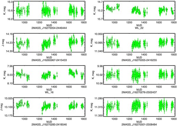
Figure 28. J or Ks light curves for eight irregular variables.
Download figure:
Standard image High-resolution image
Figure 29. J or Ks light curves for eight irregular variables.
Download figure:
Standard image High-resolution image
Figure 30. Ks light curves for eight irregular variables.
Download figure:
Standard image High-resolution image
Figure 31. J or Ks light curves for the eight irregular variables.
Download figure:
Standard image High-resolution imageTable 8. Irregular Variables
| Catalog IDa | ΔKs | Δ(J − H)b | Δ(H − Ks)c | YSO Class | Var Mech |
|---|---|---|---|---|---|
| (mag) | (mag) | (mag) | |||
| 65576–2508150 | 0.114 | 0.150 | 0.123 | — | Unknown |
| 65699–2455192 | 0.167 | 0.153 | 0.180 | — | Unknown |
| WL 21 | 0.166 | — | — | II | Unknown |
| 65744–2452589 | 0.160 | 0.105 | 0.139 | — | Unknown |
| 65789–2452371 | 0.854 | — | — | — | Unknown |
| 65789–2457518 | 0.108 | 0.093 | 0.124 | — | Unknown |
| 65861–2446029 | 0.131 | 0.198 | 0.168 | — | Accretion? |
| ISO-Oph 87 | 0.294 | 0.241 | 0.180 | II | 2 "flare" events |
| 70054–2446444 | 1.109 | — | — | — | Unknown |
| WL 22 | 0.631 | — | — | I | Unknown |
| 65967–2415433 | 0.078 | 0.124 | 0.073 | — | Unknown |
| 70055–2416255 | 0.061 | 0.082 | 0.066 | — | Unknown |
| WL 16 | 0.082 | 0.083 | 0.176 | — | Unknown |
| 70276–2502437 | 0.053 | 0.062 | 0.083 | — | Unknown |
| 70285–2418546 | 0.060 | 0.086 | 0.064 | — | Unknown |
| 70501–2508484 | 0.052 | 0.084 | 0.077 | — | Unknown |
| 70516–2420077 | 0.049 | 0.079 | 0.078 | — | Unknown |
| 70591–2459376 | 0.044 | 0.078 | 0.055 | — | Unknown |
| 70597–2428363 | 0.182 | — | 0.157 | II | Unknown |
| 60819–2442286 | 0.069 | 0.061 | 0.195 | — | Unknown |
| 71003–2429133 | 0.334 | — | 0.366 | II | Unknown |
| 71096–2445298 | 0.056 | 0.073 | 0.074 | — | Unknown |
| 71173–2447109 | 0.069 | 0.079 | 0.074 | — | Unknown |
| ISO-Oph 116 | 0.155 | 0.085 | 0.090 | II | Accretion |
| 71377–2505450 | 0.059 | 0.065 | 0.091 | — | Unknown |
| 71384–2415441 | 0.205 | — | 0.291 | — | Unknown |
| 71404–2415096 | 0.109 | 0.200 | 0.149 | — | Unknown |
| 71531–2415515 | 0.069 | 0.099 | 0.088 | — | Unknown |
| 71605–2415039 | 0.352 | — | 0.534 | — | Unknown |
| 71604–2416163 | 0.391 | — | 0.517 | — | Unknown |
| 71744–2413079 | 0.155 | 0.217 | 0.315 | — | Unknown |
| YLW 13B | 0.215 | 0.276 | 0.158 | II | Accretion |
| ISO-Oph 131 | 0.050 | 0.184 | 0.069 | III | Unknown |
| 72330–2507282 | 0.700 | — | 0.751 | — | Unknown |
| 72325–2448357 | 0.074 | 0.099 | 0.094 | — | Unknown |
| ISO-Oph 138 | 0.326 | 0.432 | 0.175 | II | Unknown |
| 73052–2432347 | 0.070 | 0.075 | 0.082 | — | Unknown |
| 73107–2504004 | 1.057 | — | — | — | Unknown |
| 73122–2504172 | 0.566 | 0.386 | 0.473 | — | Unknown |
| 73208–2508545 | 0.613 | 0.318 | 0.679 | — | Unknown |
Notes. aThe catalog ID has been truncated by 2MASS J162 for 2MASS catalog stars. bEntries with — mark stars with photometry below the survey J band completeness limit. cEntries with — mark stars with photometry below the survey H band completeness limit.
Download table as: ASCIITypeset image
The ΔKs amplitude range from 0.04 to 1.11 mag, with a median value of 0.14 mag. The Δ(H − Ks) color amplitude range from 0.05 to 0.75 mag with a median value of 0.14 mag. Using the variability criteria, discussed in Section 5, the primary variability mechanism is only identified for 4 irregular variables (2MASSJ16265861−2446029, ISO-Oph 116, YLW 13B, ISO-Oph 87). The first three exhibit a long time-scale variation in at least one observing season where the star becomes bluer as it dims. This is indicative of variable mass accretion as the variability mechanism. These stars are not considered LTVs as this variability is not the largest amplitude variability in the time-series. The variable accretion for YLW 13B is identified to occur for ∼115 days in the second year with a ΔKs ∼ 0.15 mag and Δ(H − Ks) 0.11 mag (see Figure 30). ISO-Oph 116 varies via variable accretion at least twice (see Figure 28). The first time occurs for ∼170 days in the first year with ΔKs 0.14 mag and Δ(H − Ks) 0.07 mag. The second time occurs for ∼70 days in the third year with ΔKs ∼ 0.11 mag and Δ(H − Ks) 0.07 mag. The average error in both Ks and (H − Ks) is 0.01 mag for both YLW 13B and ISO-Oph 116. In the case of 2MASSJ16265861−2446029, only the (J − H) color becomes bluer making the mechanism identification tentative. The YSO classification for this star is unknown. The J band photometry is too dim in 11 irregular variables to identify the variability mechanism. Of these 11 variables, the H band is also too dim in 5 stars.
The variability in ISO-Oph 87 is peculiar due to two flare-like events that occur in the Ks photometry on approximately 1400 and 1700 2MASS MJD. Figure 32 contains the Ks, (J − H), and (H − Ks) photometry for this Class II YSO. If the events are truly related to an increase in stellar activity, the star is expected to become bluer in both (J − H) and (H − Ks). However, no change is seen in the (J − H) color and the star reddens in (H − Ks). The first event lasts for ∼10 days with ΔKs 0.20 mag and Δ(H − Ks) 0.13 mag. The second event occurs for ∼6 days and ΔKs 0.18 mag and Δ(H − Ks) 0.16 mag. Two additional, lower amplitude spikes in the Ks photometry between 1600 and 1700 2MASS MJD might also be similar flare-like events.
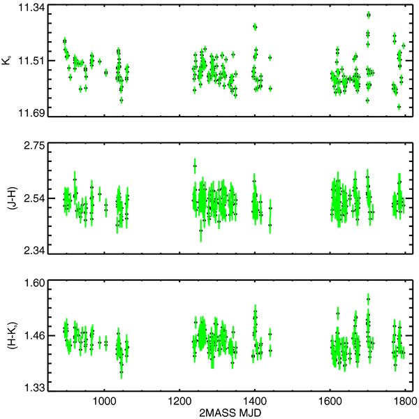
Figure 32. Ks, (J − H) and (H − Ks) photometry for ISO-Oph 87. The photometry contains at least two "flare" events, where the star brightens sharply in Ks, occurring at 1400 and 1700 2MASS MJD. Two other possible "flare" events occur between 1600 and 1700 2MASS MJD. The events become redder as the star brightens rather than becoming bluer as expected for stellar flares.
Download figure:
Standard image High-resolution imageIrregular variables have the smallest percentage (68%) of stars located "on cloud." Only nine stars in this sub-category are classified as a YSO: one Class I (8%), seven Class II (21%) and one Class III (9%).7 Most (16 stars) of the 22 candidate ρ Oph members are irregular variables. If these candidate members are YSOs then the fraction of YSO irregular variables is comparable to the fraction of periodic and LTV YSOs.
5.4. Examples of Multiple Variability Mechanisms
As discussed in the Introduction, variability studies indicate young stars sometimes exhibit complex photometric behavior believed to result from multiple variability mechanisms acting concurrently. For most stars in this survey, only the highest amplitude variability can be confidently characterized. However, a lower amplitude, second type of variability is definitely seen in seven variable stars. Four of these seven stars (YLW 1C, 2MASS J16272658−2425543, YLW 10C, WL 4) show evidence for two separate, yet statistically distinct periodic variations. The remaining three stars (WL 20W, ISO-Oph 126, WL 15) are periodically variable underneath a higher amplitude, long time-scale variation. The methods used to identify both the primary and secondary variabilities in these stars is discussed in Section 4.1. The following subsections contain detailed discussions for each of these stars except WL 4 which is described in Plavchan et al. (2008).
- 1.YLW 1C (ISO-Oph 86): This CTTS exhibits both sinusoidal-like and eclipse-like periodic variability at two distinct periods; the periods are distinct from each other to a 20σ confidence level. Figure 33 contains the Ks, (J − H) and (H − Ks) photometry folded to the sinusoidal-like period, P = 5.7792 ± 0.0085 days. The peak-to-trough ΔKs amplitude for this variability is 0.14 mag. The variability in both the (J − H) color and (H − Ks) color is not correlated with the Ks variability. This favors variability caused by rotational modulation of a cool starspot(s). Figure 34 contains the Ks, (J − H), and (H − Ks) photometry folded to the eclipse-like period, P = 5.9514 ± 0.0014 days. The ΔKs eclipse depth is 0.29 mag. The (H − Ks) color reddens during the eclipse event consistent with variability caused by extinction. This behavior is not seen in the (J − H) color. Since the J band photometry is near the survey completeness limits, the absence of a clear reddening trend may be due to low signal-to-noise ratio in the color curve.The two periods for YLW 1C is consistent with the interpretation that these events are true occultation events, as proposed for AA Tau (see Section 5.1.2). The short period, arising from a stellar surface feature(s), traces the stellar rotation rate. The longer period suggests the occultation of the star by an obscuration located just beyond the circumstellar disk co-rotation radius. Following the analysis described in Section 5.1.2, the occulter of YLW 1C is located 7.2 R⋆ from the host star and the duration of the occultation is ∼6.4 hr corresponding to a minimum occulter diameter of ∼2.0 R⋆. The reader is reminded that this diameter represents the extent within the orbital path and makes no claim on any preferential occulter shape. The eclipse depth is ΔKs = 0.29 mag.The large occulter diameter argues against the direct detection of a hot protoplanet. However, recent imaging results suggest that gas giant planets maybe considerably extended in the mass accretion phase (Quanz et al. 2013; Kraus & Ireland 2012). If true in this case, this would demonstrate the existence of a hot protoplanet with a period of six days very near the peak in the period distribution for exoplanets (Wright et al. 2012). Alternatively, the event could be caused by an occultation of a warped portion of a circumstellar disk. This scenario has been proposed to explain the near- to mid-IR variability in LRLL 31 (Flaherty & Muzerolle 2010; Flaherty et al. 2013). While most YSO disk models invoke axisymmetry, objects such as YLW 1C are prompting the creation of more complex models.
- 2.2MASS J16272658−2425543: This CTTS, designated "J543" hereafter, is another star exhibiting both sinusoidal-like and eclipse-like variability with two distinctly different periods. Figure 35 contains the Ks, (J − H), and (H − Ks) photometry folded to the sinusoidal-like period, P = 1.52921 ± 0.00065 days. The peak-to-trough ΔKs amplitude for this variability is 0.20 mag. The variability in the (J − H) and (H − Ks) colors are not correlated with the Ks photometry, which favors variability caused by rotational modulation of a cool starspot. Figure 36 contains the Ks, (J − H), and (H − Ks) photometry folded to the eclipse-like period, P = 2.9602 ± 0.0013 days. The ΔKs eclipse depth is 0.17 mag. Both the (J − H) and (H − Ks) colors redden during in the eclipse event consistent with variable extinction.The physical interpretation for the observed variability is identical to that of YLW 1C. The 1.6 day period corresponds to the stellar rotation rate and the 3.0 day period arises from a periodic occultation by an asymmetry in the inner circumstellar disk. The occulter size and distance are 2.8 R⋆ and ∼3.0 R⋆. Differing from YLW 1C, the occulter for J543 is located approximately a stellar radius beyond the co-rotation radius.
- 3.YLW 10C (ISO-Oph 122): YLW 10C is the third CTTS where two distinct periods are identified. Figure 37 contains the Ks, (J − H) and (H − Ks) photometry folded to the sinusoidal-like period, P = 3.0779 ± 0.0025 days. The peak-to-trough ΔKs amplitude for this variability is 0.25 mag. Figure 38 contains the Ks, (J − H), and (H − Ks) photometry folded to the eclipse-like period, P = 2.9468 ± 0.0029 days. The ΔKs eclipse depth is 0.28 mag. Unfortunately, both the J and H photometry are below the survey completeness limits preventing the identification of either variability mechanism.Given the sinusoidal-like and eclipse-like variability is very similar to both YLW 1C and J543, the same physical interpretation is proposed for this star. However, unlike YLW 1C, the sinusoidal-like variability, presumed to trace the stellar rotation rate, has a longer period by 3.1 hr than the periodic occultations. This places the hypothetical occulter within the co-rotation radius. The size and distance to the occulter are 3.31 R⋆ and 3.75 R⋆. The occulter is located within the dust sublimation radius as computed using the formulism of Jura & Turner (1998). This formulism is only an approximation as it does not take into account dust evaporation and condensation rates, grain size, or grain composition.
- 4.WL 20W (YLW 11B, ISO-Oph 126): This CTTS is both periodically variable and variable over a long time-scale. As such, WL 20W is designated both a periodic variable and a LTV. Figure 39 contains the Ks, (J − H) and (H − Ks) photometry for this star. The long time-scale variability begins on ∼1600 2MASS MJD and has a timescale of 122 days. The ΔKs depth is 0.26 mag. Both the (J − H) and (H − Ks) colors become redder during the long time-scale variation, consistent with variable extinction. The periodic signal is not significant unless the time-series affected by the long time-scale variability is omitted from analysis by the PA (see Figure 11). Figure 40 contains the Ks, (J − H) and (H − Ks) photometry folded to the sinusoidal-like period, P = 2.1026 ± 0.0060 days. The peak-to-trough ΔKs amplitude for the sinusoidal-like variability is 0.19 mag. Neither the (J − H) nor the (H − Ks) color is correlated to the Ks variability. This favors rotational modulation by cool starspots as the variability mechanism.The variability of AA Tau has been cited as an explanation for the periodic eclipsing variables in this survey. However, recently it has been discovered that AA Tau is exhibiting a long time-scale dimming on the order of 2–3 mag in the V band (Bouvier et al. 2013). This long time-scale variation is superimposed on top of the periodic variability. Additionally, the system appears to become bluer in this dim state; a phenomenon seen in UX Ori-type variables (Grinin et al. 1991; Herbst et al. 1994). The physical interpretation for UX Ori-type variability is that the star dims due to an asymmetric optically thick occulter beyond the inner circumstellar disk. The bluer color represents a larger contribution of scattered starlight off the occulting material.This scenario is an alternative explanation than variable mass accretion for the long time-scale variation observed in WL 20W. The eclipse depth corresponds to a 2.9 mag dimming when converted to the V band by using the extinction coefficients given in Cohen et al. (1981); this is consistent with the AA Tau long time-scale variation. The (J − H) and (H − Ks) colors do become bluer during the long time-scale variation also consistent with the observations of AA Tau. Our overall interpretation for the variability in WL 20W is a central star rotating with a two day period that is occulted by a pocket of optically thick material located beyond the inner circumstellar disk.It is worth noting this star belongs to a triple system that is spatially resolved in the mid-IR. Ressler & Barsony (2001) show the most variable member is, in fact, WL 20S. They classify this source as Class I through SED fitting of mid-IR photometry. They show that WL 20E and WL 20W are nearly constant on decadal timescales whereas the flux of WL 20W increased sixfold in 15 yr. As the largest separation between these components is 366, the large aperture size in our work (4'') includes all three stars and thus cannot rule out the possibility that the measured variability arises from this southern component.
- 5.ISO-Oph 126: This WTTS is similar to WL 20W in that it exhibits both periodic variability and a long time-scale variation. ISO-Oph 126 is also designated both a periodic variable and a LTV. Figure 41 contains the Ks, (J − H), and (H − Ks) photometry for this star. The J band photometry is below the survey completeness limits. Therefore the (J − H) color is deemed unreliable for analysis. The long time-scale variation dominates the photometry prior to 1400 2MASS MJD with a time-scale of 349 days. The ΔKs depth of this variation from the continuum brightness is 0.10 mag. The (H − Ks) color becomes redder during the long time-scale variation as the star dims. This is consistent with extinction as the variability mechanism. The PA identifies a significant periodic signal when only the portion of the time-series after 1400 2MASS MJD is analyzed (see Figure 11). Figure 42 contains the Ks, (J − H), and (H − Ks) photometry folded to the sinusoidal-like period, P = 9.114 ± 0.090 days. The peak-to-trough ΔKs amplitude for the sinusoidal-like variability is 0.06 mag. The (H − Ks) color becomes bluer as Ks brightens favoring a variability mechanism of rotational modulation by accretion-induced hot starspots.While the origin of the periodic variability can be attributed to stellar surface features, the favored interpretation of extinction in this case potentially challenges the class identification as a diskless WTTS. While Barsony et al. (2005) could not provide a YSO classification for ISO-Oph 126, the authors could place an upper limit to the spectral index at ⩽−0.88. This allows for the possibility this star is Class II and surrounded by an optically thick accretion disk.One intriguing option is the occultation by a disk surrounding an orbital companion. This scenario is invoked to explain long time-scale variability in evolved star systems
 Aur (Guinan & Dewarf 2002; Kloppenborg et al. 2010; Stencel et al. 2011), EE Cep (Mikolajewski & Graczyk 1999; Graczyk et al. 2003; Mikolajewski et al. 2005; Gałan et al. 2010), and most recently in the young star system 1SWASP J140747.93−394542.6 ("J1407"; Mamajek et al. 2012. Photometric variations within the long time-scale variations are believed to arise from structure within the occulting disk. This structure may represent new planets (EE Cep (Gałan et al. 2010)), or it may represent planetary moons (J1407; Mamajek et al. 2012). It is noted that there is significant scatter in the Ks time-series during the first half of the long time-scale variation in comparison to the second half of this variation (see Figure 43). High resolution imaging or radial velocity monitoring may help to confirm the existence of a companion to ISO-Oph 126.
 - 6.WL 15 (YLW 7A, ISO-Oph 108): This star is one of the brightest at Ks ( = 7.05 mag) and the reddest (() = 4.01 mag) in the variable catalog. WL 15 is a Class I YSO. Similar to WL 20W and ISO-Oph 126, this star exhibits a large amplitude, long time-scale variation over-top of a smaller amplitude periodic variability. Unlike WL 20W and ISO-Oph 126, the photometry during the long time-scale variation is too sparse to confidently identify a time-scale. Therefore, WL 15 is only designated a periodic variable. Figure 44 contains the Ks, (J − H), and (H − Ks) photometry for WL 15. The J band photometry is below the survey completeness limit and is deemed unreliable for analysis. The long time-scale variation is observed between 1396 and 1443 2MASS MJD with a ΔKs amplitude of ∼1 mag. The mean (H − Ks) color does not change as the star dims during this event. Even including the long time-scale variation, the PA found a significant periodic signal. Figure 45 contains the Ks, (J − H), and (H − Ks) photometry for WL 15 folded to the sinusoidal-like period, P = 19.412 ± 0.085 days. This variability has a peak-to-trough ΔKs amplitude of 0.90 mag. The (H − Ks) color is not correlated to the Ks photometry.While the colorless periodic variability favors rotational modulation by cool starspots, the amplitude of variability does not. The highest amplitude variability confirmed to be caused by cool starspots, to date, is ΔV = 0.63 mag (Strassmeier et al. 1997). This amplitude is nearly 0.3 mag lower than that observed for WL 15. In addition, the contrast between the starspot and surrounding photosphere increases toward bluer wavelengths. Therefore, the amplitude will be even larger in the optical. The origin behind the long time-scale variation is equally peculiar. As the (H − Ks) color does not become redder as the star dims, this seems to eliminate extinction as a variability mechanism. However, variability by rotational modulation of surface features seems implausible given the timescale and amplitude of the variation.


Figure 33. Ks, (J − H), and (H − Ks) photometry for YLW 1C phased to the 5.7752 ± 0.0085 day sinusoidal-like period. The red line indicates the mean value in each panel. The lack of color correlation with ΔKs points to rotational modulation of cool starspots as the variability mechanism.
Download figure:
Standard image High-resolution image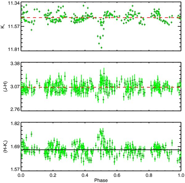
Figure 34. Ks, (J − H), and (H − Ks) photometry for YLW 1C phased to the 5.9514 ± 0.0014 day eclipse-like period. The red line indicates the mean value in each panel. Both colors become redder as Ks dims indicating variable extinction as the likely variability mechanism.
Download figure:
Standard image High-resolution image
Figure 35. Ks, (J − H), and (H − Ks) photometry for J543 phased to the 1.52921 ± 0.00065 day sinusoidal-like period. The red line indicates the mean value in each panel. The lack of color correlation with ΔKs points to rotational modulation of cool starspots as the variability mechanism.
Download figure:
Standard image High-resolution image
Figure 36. Ks, (J − H), and (H − Ks) photometry for J543 phased to the 2.9602 ± 0.0013 day eclipse-like period. The red line indicates the mean value in each panel. Both colors become redder as Ks dims indicating variable extinction as the likely variability mechanism.
Download figure:
Standard image High-resolution image
Figure 37. Ks, (J − H), and (H − Ks) photometry for YLW 10C phased to the 3.0779 ± 0.0025 day sinusoidal-like period. The red line indicates the mean value in each panel. The lack of reliable J and H photometry prohibits a confident estimate of the variability mechanism.
Download figure:
Standard image High-resolution image
Figure 38. Ks, (J − H), and (H − Ks) photometry for YLW 10C phased to the 2.9468 ± 0.0029 day eclipse-like period. The red line indicates the mean value in each panel.
Download figure:
Standard image High-resolution image
Figure 39. Ks, (J − H), and (H − Ks) photometry for WL 20W. The long time-scale variation is easily seen beginning at ∼1600 2MASS MJD. Both the (J − H) and (H − Ks) become redder as Ks dims, indicating variable extinction as the likely variability mechanism.
Download figure:
Standard image High-resolution image
Figure 40. Ks, (J − H), and (H − Ks) photometry for WL 20W folded to the period 2.1026 days. The red line indicates the mean value in each panel. No correlation between ΔKs and the change in colors points to rotational modulation of cool starspots as the likely variability mechanism. Only the photometry before the time-scale variation is plotted.
Download figure:
Standard image High-resolution image
Figure 41. Ks, (J − H), and (H − Ks) photometry for ISO-Oph 126. The long time-scale variation is easily seen prior to ∼1400 2MASS MJD. Both the (J − H) and (H − Ks) become redder as Ks dims, indicating variable extinction as the likely variability mechanism.
Download figure:
Standard image High-resolution image
Figure 42. Ks, (J − H), and (H − Ks) photometry for ISO-Oph 126 folded to the period 9.114 days. The red line indicates the mean value in each panel. The (H − Ks) color becomes bluer as Ks brightens favoring a variability mechanism of rotational modulation by accretion-induced hot starspots.
Download figure:
Standard image High-resolution image
Figure 43. Ks and (H − Ks) photometry for the long time-scale variation in ISO-Oph 126. The Ks shows considerable structure during ingress, but is nearly stable during the "eclipse" egress. The red line indicates the mean magnitude of the continuum photometry.
Download figure:
Standard image High-resolution image
Figure 44. Ks, (J − H), and (H − Ks) photometry for WL 15. The ∼19 day period is clearly evident and appears to continue even through a ∼1 mag drop in Ks band flux. The photometry during the larger amplitude flux decrease is too sparse to confidently determine a time-scale. A lack of a trend in the (H − Ks) color during this event highly suggests against extinction except by an opaque occulter.
Download figure:
Standard image High-resolution image
Figure 45. Ks, (J − H), and (H − Ks) photometry for WL 15 folded to the period 19.412 days. The red line indicates the mean value in each panel.
Download figure:
Standard image High-resolution image6. SUMMARY
High precision, high cadence J, H, Ks photometry is obtained for 7815 stars in the direction of the ρ Oph molecular cloud with a temporal baseline of ∼2.5 yr. Spurious detections, partially resolved doubles or galactic contamination are eliminated from the photometry. The target sample meeting the specifications for time-series variability analysis includes 1678 stars. A seven-point variability test is used to identify 101 variable stars, which is 6% of the parent sample. These tests are sensitive to variability on a variety of different time-scales and forms (e.g., sinusoidal, "eclipse-like," etc.).
Of the 101 stars in the variable catalog, 15% are located "on cloud" while only 1% lie within the "field." Location "on cloud," variability, and (H − Ks) colors redder than a 3 Myr isochrone are used to estimate membership in the ρ Oph star forming region. This method has identified 22 stars as previously unknown candidate ρ Oph members.
The effects of observing strategy on variability detection and measured amplitudes is investigated by comparing this work to the ρ Oph variability study performed by Alves de Oliveira & Casali (2008). These two studies have 464 stars in common; AC08 identified 7% as variable stars and this work identifies 18%. The increase in detection fraction is not caused by different sensitivities in the separate variability criteria used in each survey. This work also found both a higher Ks and (H − Ks) color amplitude in 25 stars identified as variable in both surveys than measured by AC08. Therefore a high cadence observational strategy will discover more variables within a given set of stars and it will more accurately characterize intrinsically higher amplitude variability.
The Ks variability and stellar color behaviors are used to estimate the physical mechanism responsible for the variability. Rotational modulation by long-lived cool starspots is expected to produce colorless, periodic variability. Rotational modulation of long-lived hot starspots (e.g., accretion) is, also, expected to be periodic, while short-lived starspots (e.g., flares) is not. The star becomes bluer as it brightens in both cases. Extinction induced variability is either periodic or exists on long time-scales based on the geometry of the occulter relative to the star. Changes in the mass accretion rate onto the star is not expected to be periodic, but occur on time-scales ranging from days to years. As this rate changes, the star becomes bluer as the star dims.
Identifying periodic variability within the variable catalog is done via a newly improved period-searching algorithm, the Plavchan algorithm. The algorithm tests tens of thousands of periods with uniform frequency sampling between 0.1 to 1000 days. This is done by comparing the observed light curve to a dynamically generated prior. The statistical significance of individual periods is computed via two methods: the distribution of power values at other periods in the same periodogram and the distribution of maximum power values for all sources in an ensemble survey. The Plavchan algorithm finds periodic variability in 32% of the variable catalog with periods ranging from 0.49 to 92 days.
The periodic variables are split into two sub-categories: sinusoidal-like and eclipse/inverse eclipse-like. Sinusoidal-like periodic variability describes a sinusoidal-like change in the observed flux when the time-series is folded to the most significant period. Rotational modulation by cool starspots is believed to be the common variability mechanism in this sub-category. Sinusoidal-like periodic variables are found in each YSO class (three Class I, eight Class II, eight Class III). Eclipse-like periodic variability results in discrete drops, or "dips," in the observed flux when the time-series is folded to the most significant period. Periods range from two to eight days with the duration of these dips lasting less than 30% of one periodic epoch. This sub-category contains six stars with a median peak-to-trough ΔKs and Δ(H − Ks) color amplitudes of 0.31 and 0.11 mag, respectively. Variable extinction is the likely mechanism for the eclipse-like variations. All stars in this sub-category are Class II YSOs. The inverse-eclipse-like variables, WL 4 and YLW 16A have periods of 65.61 and 92.3 days, respectively. The variability mechanism proposed in both cases is the periodic obscuration of one component in a close binary by a warped circumbinary disk.
In half of the eclipse-like variables (YLW 1C, 2MASS J16272658−2425543, YLW 10C) an additional statistically significant period is identified. This sinusoidal-like periodic variability coupled with the presence of "dips" suggests a rapidly rotating spotted star occulted by a clump of optically thick material in the inner accretion disk. These stars strengthen the interpolation posed to explain the variability of other YSO AA Tau-like variables (Morales-Calderón et al. 2011). The periods corresponding to periodic occultations in YLW 1C and YLW 10C are located near their respective co-rotation radii. The mechanism driving these occultations could arise from a warped inner circumstellar disk caused by an inclined magnetic dipole, or could be the pre-natal cloud of a forming hot Jupiter.
Long time-scale variables is a variability subclass, containing 31 stars, where the measured flux increases or decreases consistently over months or years. The variability time-scale is measured using a differencing technique and approximates the time between maximum and minimum brightness. The measured time-scales range from 64 to 790 days. The peak-to-trough ΔKs amplitudes range from 0.05 to 2.31 mag and the peak-to-trough Δ(H − Ks) color amplitudes range from 0.06 to 1.32 mag. Variable extinction and variable accretion rates are both equally likely to cause long time-scale variability. This subclass contains 25 known YSOs with 7 Class I, 15 Class II and 3 Class III stars.
The time-series of irregular variables are aperiodic and do not vary over any discernible time-scale. This subclass contains more members (40) than either the periodic or long time-scale subclasses. The peak-to-trough ΔKs amplitudes range from 0.04 to 1.11 mag and peak-to-trough Δ(H − Ks) color amplitudes range from 0.05 to 0.75 mag. No single dominant variability mechanism explains irregular variability. Only nine known YSOs (one Class I, seven Class II, one Class III) are irregular variables.
The CTTS WL 20W and the WTTS ISO-Oph 126 are similar in both have a long time-scale variation superimposed onto a periodic signal. In both cases, the physical mechanisms for the variability is consistent with an occultation of a rapidly rotating spotted star by optically thick material outside the inner accretion disk. For WL 20W, the sinusoidal-like variability has a period of 2.1026 days and a peak-to-trough ΔKs amplitude of 0.19 mag. The long time-scale variability has a duration of 122 days with a ΔKs eclipse depth of 0.26 mag. For ISO-Oph 126, the sinusoidal-like variability has a period of 9.114 days and a peak-to-trough ΔKs amplitude of 0.06 mag. The long time-scale variability has a duration of 349 days with a ΔKs eclipse depth of 0.10 mag.
The very high amplitude periodic variability measured in the Class I star WL 15 is not consistent with any proposed mechanism. The observed 47 day colorless decrease in Ks band brightness of ∼1 mag is also not easily estimated.
From cross-referencing the target sample with two previous surveys, 72 stars have been assigned a YSO classification (13 Class I, 47 Class II, 12 Class III). The variability fraction of these YSOs is 79%. The variability fraction differs according to YSO class with 92% of Class I and Class III stars identified as variable; this fraction drops to 72% for Class II stars. The amplitude of both brightness and color variability are decreasing functions of YSO class. The median peak-to-trough ΔKs amplitude for Class I, II and III stars are 0.77, 0.31, and 0.08 mag, respectively. In addition, the median peak-to-trough Δ(H − Ks) color amplitudes are 0.81, 0.21, and 0.07 mag for each class respectively.
We express our thanks to our anonymous referee for conversation and comments. We also express our thanks to Mary Barsony for her many insightful questions and suggestions. This publication makes use of data products from the Two Micron All Sky Survey, which is a joint project of the University of Massachusetts and the Infrared Processing and Analysis Center/California Institute of Technology, funded by the National Aeronautics and Space Administration and the National Science Foundation. This research has made use of the NASA Exoplanet Archive, which is operated by the California Institute of Technology, under contract with the National Aeronautics and Space Administration under the Exoplanet Exploration Program. The authors would like to acknowledge the Infrared Processing and Analysis Center's Visiting Graduate Student program for providing the opportunity and funding for this publication.
APPENDIX: EMPIRICAL DETERMINATION OF DEPENDENCE ON PARAMETERS

In this Appendix an analysis of the dependence of the PA periodogram χ power values on the number of observations and periodogram parameters n0 and p is presented. The ensemble survey of mostly non-variable stars is used to carry out this analysis and to present an alternative approach to evaluate the statistical significance of periodogram power values.

First, a random subset of 180 stars is chosen from the survey collection of 1678 stars. These stars are evenly distributed in Nobs and Ks magnitude. For a given set of parameters, p and n0, the maximum χ periodogram power value is computed for the 180 stars. Since other algorithms exist that specialize in finding periodic sources with low numbers of detection (Dworetsky 1983, Nobs ∼ 20), test cases are limited to 0.04 < p and ⩽0.5 and 12 < n0 ⩽ 250. Figure 46 shows the dependence of on Nobs for the 180 stars with a particular set of p and n0. This dependence is somewhat expected—a smaller number of observations can result in an increase in the likelihood of false-positive periodogram peaks.


Figure 46. Graph of the χ value as a function of detection size, Nobs, for the test case with the parameters: n0 = 25 and p = 0.06. The red line represents the functional fit of Equation (A1) with values of (a, b, c) = (62.5495, 18.4963, 1.2523) where the residuals are minimized.

Download figure:
Standard image High-resolution imageThe distribution of χ values as a function of Nobs is well-described by the functional form:


where a, b and c represent real numbers that differ for a given p and n0. As the power law index decreases below 1.5 for p < 0.04 and/or n0 < 12, these ranges are excluded from the analysis. Equation (A1) is found via trial and error to minimize the residuals when compared to a variety of functional forms tested, rather than from an analytic derivation based upon first principles.
The next step is to determine how the constants a, b, and c vary as functions of the parameters p and n0. Fixing n0, the maximum χ as a function of Nobs is empirically fit to 10 chosen p values resulting in 10 different values of a, b, and c. The same process is repeated except p is fixed and n0 is varied. Figure 47 displays the dependence of a on the parameters p and n0. Six fits to the dependence of a, b, and c on parameters p and n0 are determined empirically through trial and error to be:


The particular functional forms of Equations (A2) and (A3) are again not analytically motivated, but instead minimize the residuals from a variety of functional forms tested.

Figure 47. Top: graph of the constant a as a function of parameter p (see Equation (A3a)). Bottom: graph of the constant a as a function of parameter n0 (see Equation (A2a)).
Download figure:
Standard image High-resolution imageThese six functions of one parameter are combined into three functions of both parameters p and n0. This is accomplished by replacing the constant term in the n0 function by the entire corresponding p function. The constant term from the fc(p) function is also dropped. Thus, the following functions are found to adequately describe the dependence of a, b, and c on parameters p and n0 for this survey:


and therefore Equation (A1) can be rewritten as:

The values p and n0 = 40—used throughout this paper to identify periodic variables – are an optimal choice of parameters for this survey. They yield the smallest residuals when the 180 test cases are fit in Equation (A5). Thus, for this survey the maximum peak power in the periodogram for a non-variable star is approximately given by the expression:

The validity of the numerical fits (Equations (A4a)–(A4c)) is verified using an additional 18 test cases with randomly selected values of p and n0. The χ versus Nobs distributions are again fit using Equation (A1), yielding 18 "observed" a, b, and c values for each pair of p and n0. Predicted values for a, b and c are found by using Equations (A4a)–(A4c) and comparing these values to the "observed" values. The mean percent errors between the observed and predicted values for the 18 test cases are −1.1 ± 3.4% for fa, 1.1 ± 3.5% for fb and −0.1 ± 1.8% for fc. Table 9 contains the percent errors for each of the individual 18 test cases. Equations (A4a)–(A4c) therefore adequately predict the values a, b, and c in Equation (A1) for any set of parameters p and n0 within the parameter space explored in this survey. Thus, this demonstrates that the PA algorithm is reasonably "well-behaved." Equation (A5) could be applied to different surveys and cadences. However, the particular numerical values in Equations (A4) and (A6) for a, b, and c likely depend on the specific cadence of a survey.

Table 9. Monte Carlo Simulation: Testing Significance Function
| n0 | p | Obs. Param. A | Pred. Param. A | % Errora | Obs. Param. B | Pred. Param. B | % Errora | Obs. Param. C | Pred. Param. C | % Errora |
|---|---|---|---|---|---|---|---|---|---|---|
| 12 | 0.25 | 31.338 | 30.382 | −3.054 | 6.796 | 6.574 | −3.259 | 1.205 | 1.239 | 2.815 |
| 13 | 0.04 | 80.893 | 76.952 | −4.872 | 22.235 | 23.263 | 4.622 | 1.393 | 1.372 | −1.500 |
| 15 | 0.06 | 64.109 | 65.547 | 2.243 | 17.776 | 18.042 | 1.500 | 1.308 | 1.307 | −0.042 |
| 18 | 0.05 | 69.756 | 70.192 | 0.625 | 19.958 | 20.568 | 3.054 | 1.310 | 1.309 | −0.054 |
| 18 | 0.06 | 63.138 | 65.036 | 3.006 | 18.173 | 18.284 | 0.610 | 1.287 | 1.290 | 0.208 |
| 25 | 0.06 | 62.550 | 64.284 | 2.772 | 18.496 | 18.560 | 0.343 | 1.253 | 1.257 | 0.337 |
| 25 | 0.40 | 25.656 | 25.169 | −1.898 | 5.833 | 5.565 | −4.602 | 1.135 | 1.148 | 1.136 |
| 25 | 0.10 | 49.530 | 48.938 | −1.194 | 13.192 | 13.411 | 1.662 | 1.200 | 1.219 | 1.602 |
| 25 | 0.04 | 79.775 | 75.265 | −5.653 | 22.927 | 24.024 | 4.784 | 1.290 | 1.310 | 1.534 |
| 40 | 0.06 | 62.172 | 63.863 | 2.719 | 18.604 | 18.693 | 0.479 | 1.208 | 1.210 | 0.194 |
| 60 | 0.24 | 29.562 | 28.859 | −2.378 | 8.219 | 7.796 | −5.145 | 1.128 | 1.092 | −3.168 |
| 75 | 0.055 | 68.359 | 66.993 | −1.998 | 18.500 | 19.682 | 6.390 | 1.157 | 1.174 | 1.423 |
| 125 | 0.30 | 28.994 | 27.429 | −5.397 | 6.329 | 6.666 | 5.334 | 1.080 | 1.055 | −2.269 |
| 140 | 0.45 | 24.910 | 25.700 | 3.171 | 5.127 | 5.144 | 0.335 | 1.067 | 1.036 | −2.884 |
| 175 | 0.14 | 43.597 | 40.392 | −7.351 | 10.569 | 10.796 | 2.143 | 1.090 | 1.092 | 0.145 |
| 180 | 0.05 | 71.813 | 70.318 | −2.082 | 20.056 | 20.808 | 3.751 | 1.147 | 1.168 | 1.867 |
| 200 | 0.06 | 63.461 | 65.170 | 2.694 | 18.439 | 18.522 | 0.451 | 1.145 | 1.149 | 0.385 |
| 240 | 0.40 | 26.132 | 26.062 | −0.268 | 5.800 | 5.525 | −4.742 | 1.070 | 1.040 | −2.794 |
Note. aNegative % errors indicates the significance function underestimates the actual value.
Download table as: ASCIITypeset image
To evaluate the statistical significance of a peak period power value in a periodogram, it does not suffice to identify the expected value for the ensemble survey. The scatter about the expected value is also necessary. This scatter, or standard deviation (σ), of the peak period power values about the expected value depends on Nobs in a predictable fashion for this survey (Figure 48). To characterize this scatter, the scatter for each survey star is grouped into bins as a function of Nobs, with a bin size of 25. An average σ is computed for each bin and an empirical fit to this distribution is made, given by Equation (A7):


Figure 48. Maximum PA periodogram power value for a star in this survey is found to be well-described by Equation (A5) (Figure 46). The scatter about the value predicted by Equation (A5), σ, is also found to be dependent on Nobs as shown in this figure.
Download figure:
Standard image High-resolution image
Figure 49.
Light and color curves for all stars in the variable catalog. For periodic variable stars, the light and color curves folded to the appropriate period are also shown. (A color version and the complete set (271 figures) of this figure are available in the online journal.)
Download figure:
Standard image High-resolution imageAn affirmative periodicity condition can now be defined by putting it all together. The statistical significance of a measured period for a star in this survey is simply a function of the number of observations. Based on visual inspection of star light curves, this condition is defined by the following:

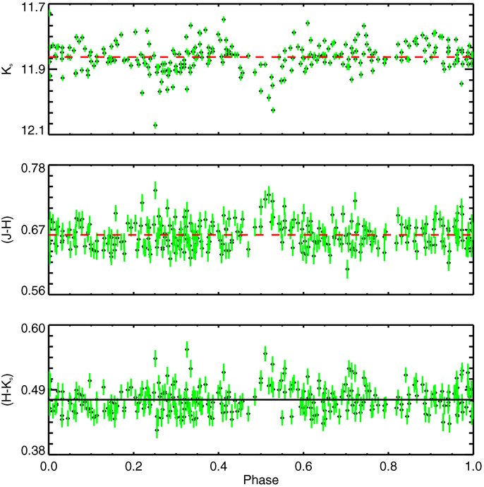
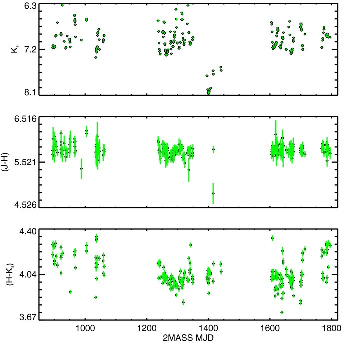
Periods where this condition is met can be considered statistically significant for the star investigated. Periods found using this criteria are generally also found to be statistically significant using the methods outlined in Section 4.1.
Footnotes
- 3
The correlations between stellar color and brightness are based on models in Carpenter et al. (2001 and references herein).
- 4
The percentages indicate the percentage of variable stars in each class that are sinusoidal-like periodic variables.
- 5
The percentage indicates the percentage of variable Class II stars that are eclipse-like periodic variables.
- 6
The percentages indicate the percentage of variable stars in each class that are sinusoidal-like periodic variables.
- 7
The percentages indicate the percentage of variable stars in each class that are irregular variables.