


ABSTRACT
In this catalog we present the updated set of spectral analyses of gamma-ray bursts (GRBs) detected by the Fermi Gamma-Ray Burst Monitor during its first four years of operation. It contains two types of spectra, time-integrated spectral fits and spectral fits at the brightest time bin, from 943 triggered GRBs. Four different spectral models were fitted to the data, resulting in a compendium of more than 7500 spectra. The analysis was performed similarly but not identically to Goldstein et al. All 487 GRBs from the first two years have been re-fitted using the same methodology as that of the 456 GRBs in years three and four. We describe, in detail, our procedure and criteria for the analysis and present the results in the form of parameter distributions both for the observer-frame and rest-frame quantities. The data files containing the complete results are available from the High-Energy Astrophysics Science Archive Research Center.
Export citation and abstract BibTeX RIS
1. INTRODUCTION
During its first four years of operation, the Fermi Gamma-Ray Burst Monitor (GBM; Meegan et al. 2009) provided the scientific community with an enormous sample of gamma-ray burst (GRB) data, significantly expanding our understanding of the physical properties and characteristics of GRBs. In addition, discoveries of new and intriguing phenomena were associated with many individual GRBs (e.g., Ackermann et al. 2010; Guiriec et al. 2011; Ackermann et al. 2011; Axelsson et al. 2012; Guiriec et al. 2013).
Here, we present the second GBM GRB spectral catalog which will provide the most comprehensive resource of GRB spectral properties to date. In order to be as complete and uniform as possible, our methodology follows closely, but is not identical to, the procedures employed in the GRB catalog from the Burst And Transient Source Experiment (BATSE; Kaneko et al. 2006) and the first GBM GRB spectral catalog (Goldstein et al. 2012). We include representative spectral fits for all GBM bursts from the first four years of operation (2008 July 14–2012 July 13).
For each GRB, we show two types of spectra: time-integrated spectra (henceforth labeled F for fluence) and spectra at the brightest time bin (henceforth labeled P for peak flux). A set of four empirical models was applied to the data in both cases. The selection of these model functions is based on tradition (Band et al. 1993; Kaneko et al. 2006; Goldstein et al. 2012) and mathematical complexity. The signal-to-noise ratios (S/Ns) in the data of GBM bursts rarely support models with more than four free parameters, which is why we resort to models with two, three or four free fit parameters and only in exceptional cases additive terms (e.g., a blackbody component; Axelsson et al. 2012) can be added. Making use of the Castor statistics (Ackermann et al. 2011), we derive the best model for each GRB and present the distribution and characteristics of the model parameters.
This catalog is organized as follows. In Section 2 we present a short overview of the GBM; in Section 3 we describe the methodology used in the production of this catalog, including detector selection, data types, energy selection and background fitting, and the source selection. We then offer a description of the spectral models used in this catalog in Section 4, present the spectral analysis methods in Section 5, and present the results in Section 6. Finally, in Section 7 we conclude with a summary and a discussion.
2. FERMI GBM
The Fermi 14 Gamma-Ray Space Telescope was successfully launched on 2008 June 11 into a Low Earth orbit of ∼565 km altitude at an 25 6 inclination. Its payload comprises two instruments, the GBM and the Large Area Telescope (LAT; Atwood et al. 2009). The goal of GBM is to augment the science return from Fermi with its prime objective being joint spectral and timing analyses of GRBs seen in common with the LAT. In addition, GBM provides near real-time burst locations which permit (1) the Fermi spacecraft to repoint the LAT toward the observed GRB and (2) to perform follow-up observations with ground-based facilities. Compared to other high-energy spacecraft, the great advantage of GBM is its capability to observe the whole unocculted sky at any given time with a field of view of ⩾8 sr and its very broad energy coverage. Therefore, along with GRBs, GBM offers great capabilities to observe all kinds of high-energy astrophysical phenomena, such as, e.g., solar flares (e.g., Gruber et al. 2011b; Ackermann et al. 2012a), soft gamma repeaters (e.g., Lin et al. 2011; von Kienlin et al. 2012) and terrestrial gamma-ray flashes (e.g., Briggs et al. 2013).
Designed to study the gamma-ray sky in the energy band of ∼8 keV–40 MeV, GBM is composed of 12 sodium iodide (Na i) and two bismuth germanate (BGO) scintillation detectors. With a thickness of 1.27 cm and a diameter of 12.7 cm, the Na i crystals cover an energy range from 8 keV–1 MeV. They are oriented around the spacecraft such that the position of the GRB can be determined.
The two BGO crystals have a diameter and thickness of 12.7 cm, covering an energy range of 200 keV–40 MeV, and are located on opposite sides of the spacecraft so that at least one is illuminated from any direction. A source location is calculated in spacecraft coordinates and used in the production of the detector response matrices (DRMs; see Section 5).
For more details on the GBM detectors and their calibration, refer to Meegan et al. (2009), Bissaldi et al. (2009), and Paciesas et al. (2012).
3. METHOD
During the first four years of operation, GBM triggered on a total of 954 GRBs (von Kienlin et al. 2014), 943 of which are presented in this catalog. The remaining bursts are excluded due to a low accumulation of counts or a lack of spectral/temporal coverage. In order to deliver the most useful analysis to the community, we have attempted to make the method as systematic and uniform as possible; circumstances under which deviations were employed are clearly indicated. Details of the detector and data selection as well as the process used to fit the data are described in this section. Many of the criteria are adopted from the GBM Burst Catalog (Paciesas et al. 2012) and we have attempted to maintain this in all aspects. However, due to the nature of spectral analysis we demand stricter criteria to ensure that we have adequate signal in all energy channels. This effectively reduces the GRB sample from that used in the burst catalog.
We highlight that this catalog only presents the analysis of GRBs that triggered the GBM. There is a non-negligible amount of GRBs that did not trigger GBM whose temporal and spectral properties are presented elsewhere (Gruber et al. 2012). These GRBs do not have different properties compared to the triggered GRB sample but simply occurred during times when the GBM triggering algorithm was switched off (e.g., when the spacecraft was at latitudes of high geomagnetic activity).
3.1. Detector Selection
The detector selection is consistent with Goldstein et al. (2012), i.e., a maximum of three Na i detectors together with one BGO detector were used for the spectral analysis. Since the effective area (i.e., detection efficiency) of the Na i detectors decreases rapidly for high incidence angles (Bissaldi et al. 2009) only detectors with source angles ⩽60° are used for the spectral analysis. In addition, it has been verified that the detectors were neither obstructed by the spacecraft nor by the solar panels of Fermi. However, due to small inaccuracies in the spacecraft mass model or location uncertainties, the blockage code does not always return a subset of detectors that is free from blockage. This is evident when the low-energy data deviate strongly from the fit model (Goldstein et al. 2012). When this occurs we remove these detectors from the selected sample. If more than three Na i detectors are qualified for the spectral fitting, the Na i detectors with the smallest source angles were used to avoid a fitting bias toward lower energies.
3.2. Data Types
GBM persistently records two different types of science data, called CTIME (fine time resolution, coarse spectral resolution of 8 energy channels) and CSPEC (coarse time resolution, full spectral resolution of 128 energy channels). CTIME (CSPEC) data have a nominal time resolution of 0.256 s (4.096 s) which is increased to 64 ms (1.024 s) whenever GBM triggers on an event. After 600 s in triggered mode, both data types return to their non-triggered time resolution. The third and primary data type used in this catalog is the "time tagged events" (TTEs) which consist of individual events, each tagged with arrival time (2 μs precision), energy (128 channels) and detector number. The TTE data are generated and stored on-board in a continuously recycling buffer. When GBM enters trigger mode, the buffered pre-trigger TTE are transmitted as science data along with ∼300 s of post-trigger TTE.
For the purpose of this catalog, we choose a standard time binning of 1024 ms for bursts longer than 2 s in duration as defined by the burst T90 (Kouveliotou et al. 1993) presented in von Kienlin et al. (2014) and 64 ms for bursts of duration 2 s and shorter. The time history of TTE typically starts at ∼30 s before trigger and extends to ∼300 s after trigger. This TTE data time span is adequate for the analysis of most GRBs. For GRBs that have evident precursors or emissions that last more than 300 s after trigger, we use the CSPEC data, which extend ∼4000 s before and after the burst for triggered events. CSPEC data were used for 76 GRBs in this catalog.
3.3. Energy Selection and Background Fitting
With the optimum subset of detectors selected, the best time and energy selections are chosen to fit the data. The available and reliable energy channels in the Na i detectors lie between ∼8 keV and ∼1 MeV. This selection excludes the overflow channel at high energies and those channels <8 keV where the transmission of gamma-rays is poor due to the silicone pad in front of the Na i crystal and the multi layer insulation around the detectors (Bissaldi et al. 2009). We perform a similar selection to the BGO detector for each burst, selecting channels between ∼300 keV and ∼38 MeV. We select enough pre- and post-burst data to sufficiently model the background and fit a single energy dependent polynomial (choosing up to fourth order) to the background. For each detector the time selection and polynomial order are varied until the χ2 statistic map over all energy channels is minimized, resulting in an adequate background fit. This approach is rather subjective in that it is dependent on the observer's choice of the background intervals. In the future, it may be advantageous to implement more objective background selection methods such as the "direction dependent background fitting" method presented in Szécsi et al. (2013).
3.4. Source Selection
Knowing the background model, the background-subtracted count rates are summed over all Na i detectors for a given burst to produce a single GRB count light curve. Using this light curve, only time bins (1.024 s for long burst and 64 ms for short bursts) with an S/N greater or equal to 3.5 were selected, in agreement with Goldstein et al. (2012). This time selection is then applied to all detectors for a given burst.
This criterion ensures that there is adequate signal to successfully perform a spectral fit and constrain the parameters of the fit. This does however eliminate some faint bursts from the catalog sample (i.e., those with no time bins with signal above 3.5σ). While the possibility remains that not all signal from the GRB was selected, this method nevertheless provides the most objective way to obtain a selection of intrinsic GRB counts as including less significant bins would only increase the uncertainty in the measurements.
This selection is what we refer to as the F selection, since it is a time-integrated selection and the derived photon and energy fluences are representative of but not equal to the fluence over the total duration of the burst. We draw attention to the fact that time bins with an S/N less than 3.5, which were not included in the fitting process, also contribute to the photon and energy fluence. For more than 80% of the GRBs in the catalogue the ratio of count fluence (without the intervals with S/N < 3.5) versus the total counts (with the intervals with S/N < 3.5) is larger than 0.8. So while there are some bursts for which the fluence can be considerably underestimated, the other option would be to overestimate the fluence of those bursts by including background that contaminates the spectral fits.
The other selection performed is a 1.024 s peak photon flux selection for long bursts (T90 > 2 s) and 64 ms peak count rate flux selection for short bursts (T90 ⩽ 2 s). This selection is made by adding the count rates in the Na i detectors again and selecting the single bin of signal with the highest background-subtracted count rate. This selection is a snapshot of the energetics at the most intense part of the burst and is depicted as the P selection.
Figure 1 shows the distribution of accumulation times used for the fitting process based on the signal-to-noise selection criteria. The distribution of accumulation times reported is similar to the observed emission time of the burst, excluding quiescent periods, (e.g., Mitrofanov et al. 1999) and peaks at 0.26 s and ∼15 s for short and long GRBs, respectively. The dividing duration time scale between the two classes of GRBs is ∼1.27 s and is, as expected from the employed source selection methodology, somewhat smaller than the canonical 2 s (Kouveliotou et al. 1993). Figure 1 also includes the comparisons of the model photon fluence and model photon flux compared to the accumulation time. In both cases two specific regions are visible for long and short GRBs. In addition, Figures 1(b) and 1(c) show a clear correlation between the photon fluence (flux) and accumulation time, indicating the existence of two different burst groups, similar to the ones delineated by the hardness–duration relationship found by Kouveliotou et al. (1993).

Figure 1. Panel (a) shows the distribution of the accumulation times based on the 3.5σ signal-to-noise selections. Note the similarity to the traditional t90 distribution, with the minimum near 1 s. No other estimation of the duration was factored into the production of the accumulation time. Panels (b) and (c) show the comparison of the model photon fluence and model photon flux to the accumulation time respectively. The photon fluences and fluxes shown in these figures are from the estimated BEST model fits.
Download figure:
Standard image High-resolution image4. MODELS
We chose four spectral models to fit the spectra of GRBs in our selection sample. These models include a single power law (Pl), Band's GRB function (Band), an exponential cut-off power law (Comp), and a smoothly broken power law (Sbpl). All models are formulated in units of photon flux with energy (E) in keV and multiplied by a normalization constant A (photon s−1 cm−2 keV−1). Below we describe each model and its features in detail.
4.1. Power-law Model
The single power law with two free parameters is defined as

where A is the amplitude and λ is the spectral index. The pivot energy (Epiv) normalizes the model to the energy range under consideration and helps reduce cross-correlation of other parameters. In all cases, Epiv is held fixed at 100 keV. While most GRBs exhibit a spectral break in the GBM passband, some GRBs are too weak to adequately constrain this break in the fits. These bursts are well fit by the single power law.
4.2. Band's GRB Function
Band's GRB function (Band et al. 1993) has become the standard for fitting GRB spectra, and therefore we include it in our analysis:

The four free parameters are the amplitude, A, the low- and high-energy spectral indices, α and β, respectively, and the νFν peak energy, Epeak. This function is essentially a smoothly broken power law with a curvature defined by its spectral indices. The low-energy index spectrum is a power-law only asymptotically.
4.3. Comptonized Model
The Comptonized model is an exponentially cutoff power law, which is a subset of the Band function in the limit that β → −∞:

The three free parameters are the amplitude A, the low-energy spectral index α and Epeak. Epiv is again fixed to 100 keV, as for the power-law model.
4.4. Smoothly Broken Power Law
The final model that we consider in this catalog is a broken power law characterized by one break with flexible curvature and is able to fit spectra with sharp or smooth transitions between the low- and high-energy power laws. This model, first published in Ryde (1999), where the logarithmic derivative of the photon flux is a continuous hyperbolic tangent, has been re-parameterized (Kaneko et al. 2006) as given below:

where

In the above relations, the low- and high-energy power-law indices are λ1 and λ2, respectively, Eb is the break energy in keV, and Δ is the break scale in decades of energy. The break scale is independent and not coupled to the power-law indices as for the Band function, and represents an additional degree of freedom. However, Kaneko et al. (2006) found that an appropriate value for Δ for GRB spectra is 0.3; therefore, we fix Δ at this value. In addition, we tested the behavior of Δ for some bright GRBs by letting it vary during the fit process. The results of this study are presented in Section 6.
We choose to fit these four different functions because the measurable spectrum of GRBs is dependent on intensity. Less intense bursts (in the observer frame) provide less data to support a large number of parameters. This may appear obvious, but it allows us to determine why in many situations a particular empirical function provides a poor fit, while in other cases it provides an accurate fit. For example, the energy spectra of GRBs are normally well fit by two smoothly joined power laws. For particularly bright GRBs, the Band and Sbpl functions are typically an accurate description of the spectrum, while for weaker bursts the Comp function is most appropriate. Bursts that have signal significance on the order of the background fluctuations do not have a detectable distinctive break in their spectrum and so the power law is the most appropriate function.
5. DATA ANALYSIS
The spectral analysis of all bursts was performed using RMfit, version 4.0rc1. RMfit employs a modified, forward-folding Levenberg–Marquardt algorithm for spectral fitting which means that the aforementioned models are used as trial source spectra which are converted to predicted detector count histograms. These histograms, in turn, are then compared to the actual, observed data.
In order to work properly, a method must be established to associate the energy deposited in the detectors to the energy of the detected photons, which depends on effective area and the angle of the detector to the incoming photons. We use DRMs to convert the photon energies into detector channel energies. DRMs contain information about the effective area of the detector, effects of the angular dependence of the detector efficiency, partial energy deposition in the detector, energy dispersion and nonlinearity of the detector and, finally, atmospheric and spacecraft scattering of photons into the detector. Therefore, DRMs are functions of photon energy, measured energy, the direction to the source (with respect to the spacecraft) and the orientation of the latter with respect to the Earth. The response matrices for all GRBs in the catalog were made using GBMRSP v2.0 of the response generator and version 2 of the GBM DRM database, and all responses employ atmospheric response modeling to correct for atmospheric scattering. In particular, we use RSP2 files, which contain multiple DRMs based on the amount of slew the spacecraft experiences during the burst. A new DRM is calculated for every 2° of slew, changing the effective area of each detector based on its angle to the source. These DRMs are then all stored in a single RSP2 file for each detector. During the fitting process, each DRM is weighted by the counts fluence through the detector during each 2° slew segment.
At all times, the Castor C-Statistic (C-Stat), which is a modified log likelihood statistic based on the Cash parameterization (Cash 1979) is used in the model-fitting process as a figure of merit to be minimized. This statistic is preferable over the more traditional χ2 statistic minimization because of the non-Gaussian counting statistics present when dividing the energy spectra of GBM GRBs into 128 channels. The drawback of this statistic is that it does not provide an estimation of the goodness-of-fit, since no standard probability distribution for likelihood statistics exists. Normally, the goodness-of-fit must be estimated for the model in use. This is usually done by simulating the model many times in order to calculate a test statistic, C-Stat in this case, for each fake model of each data set. The observed value of the test statistic is then compared to the constructed fake test statistic distribution. This would allow to reject a model with a certain level of confidence. However, performing these kind of simulations is unfeasible for such a large sample of GRBs. In addition, any goodness-of-fit method can never provide a probability that any given model is the adequate representation of the burst emission, i.e., the correct model. Therefore, we refrain from performing extensive goodness-of-fit tests and present the fit parameters for each model fit, independent of the goodness-of-fit. As we only apply four different models, it can be instructive to study the fit parameters even if the model is not a perfect representation of the data. We do, however, apply additional selection criteria and employ cuts to define a GOOD and BEST sample of the obtained fit results. These are explained in the following subsections.
Finally, we caution the reader that the 1σ errors reported in this catalog are of statistical nature only. Systematic effects were not considered which generally are non-negligible. For example, for weak events a different selection of on and off intervals for the background fitting can have effects as large as 30% for the final reported value of Epeak (see also Collazzi et al. 2011).
5.1. The GOOD Sample
We classify fitted burst models as GOOD if the parameter error of all model parameters is within certain limits. This is a more conservative approach compared to Kaneko et al. (2006) and Goldstein et al. (2012) who only required the error of the parameter of interest to be within given limits. The motivation behind this new approach is to show parameter values of models which are globally well-constrained, rather than basing interpretations on constrained parameters of overall poorly constrained models. We simultaneously require for the low-energy power law an error less than 0.4, for high-energy power-law indices an error less than 1.0 and for all other parameters we require a relative error of 0.4 or less. These criteria are an arbitrary choice but are in line with other GRB catalogs (Kaneko et al. 2006; Goldstein et al. 2012). Applying these criteria, the number of bursts that classify as GOOD for each employed model can be seen in Table 2. We draw the reader's attention to the fact that for many GRBs there can be several models which qualify as GOOD.
5.2. The BEST Sample
In addition, we define a BEST sample in order to determine which of the GOOD models is the best representation of the burst emission. Besides the necessity of having constrained parameters—already required for the GOOD sample—we compare the difference in C-Stat (ΔC-Stat) per degree of freedom between the various models. In order to assess if a statistically more complex model, i.e., a model with more free fit parameters (hypothesis H1) is preferred over a simpler model (null hypothesis H0) according to its difference in C-Stat, we created a set of 5 × 10⁴ synthetic GRB spectra using the fit parameters of H0, obtained from the fit to the real data, as source counts. Similarly, the background counts of the synthesized spectra are estimated from the real data. The input source counts are then folded through the DRM. Finally, Poisson noise was added to the sum of the source and background counts. The synthetic spectra were then fitted with both models, adding Poisson fluctuations to each energy channel of the background spectrum during the fit process.
Integrating the ΔC-Stat distribution from 0% to 99.73% (i.e., a 3σ confidence interval) we identified a critical ΔC-Statcrit. If the ΔC-Stat observed in the real data exceeds this critical value, then the null hypothesis is rejected and the statistically more complex model is preferred.
As the full GRB sample contains nearly 1000 GRBs doing the aforementioned analysis for all bursts is not feasible. We used four typical bursts which are located in four energy fluence classes, separated by one order of magnitude. These bursts are GRB 120608.489, GRB 110227.240, GRB 120129.580 and GRB 120526.303 with an energy fluence [10 keV–1 MeV] of 5.2 × 10⁻⁷ erg cm−2, 1.9 × 10⁻⁶ erg cm−2, 5.8 × 10⁻⁵ erg cm−2, 1.3 × −4 erg cm−2, respectively.
For each of the aforementioned GRBs, we created a Pl versus Comp and a Comp versus Band distribution and determined the ΔC-Statcrit for each model comparison. To assess which of the four models qualifies for the BEST sample we used the critical values as a function of fluence. For the comparison between the Band and the Sbpl such simulations were not necessary, as both functions have the same number of degrees of freedom. Therefore, the model with the lower C-Stat value was used.
As there is no observable correlation between ΔC-Statcrit and the energy fluence (see Table 1) we use the average ΔC-Statcrit value, for the model selection of all bursts, i.e., for Pl versus Comp we use ΔC-Statcrit = 8.58 and for Comp versus Band we use ΔC-Statcrit = 11.83
Table 1. Determination of ΔC-Statcrit
| Burst | Fluence | ΔC-Statcrit | ΔC-Statcrit |
|---|---|---|---|
| (erg) | Pl vs. Comp | Comp vs. Band | |
| GRB 120608.489 | 5.2e−07 | 8.55 | 13.35 |
| GRB 110227.240 | 1.9e−06 | 7.75 | 9.56 |
| GRB 120129.580 | 5.8e−05 | 8.25 | 10.55 |
| GRB 120526.303 | 1.3E−04 | 9.75 | 13.85 |
| Average | ⋅⋅⋅ | 8.58 | 11.83 |
Download table as: ASCIITypeset image
The key idea for the BEST parameter sample is to obtain the best estimate of the observed properties of GRBs. By using model comparison, the preferred model is selected, and the parameters are reviewed for that model. The models contained herein and in most GRB spectral analyses are empirical models, based only on the data received; therefore the data from different GRBs tend to support different models. Perhaps it will be possible to determine the physics of the emission process by investigating the tendencies of the data to support a particular model over others. This is the motivation to provide a sample that contains the best picture of the global properties of the data, that prompts the investigation of the BEST sample.
Applying the BEST criteria we are left with 941 GRBs for the fluence spectra and 932 GRBs for the P spectra (see again Table 2). These numbers are smaller than the total number of GRBs in this catalog (943). This is due to the fact that for some bursts the spectral fit did not converge properly and these bursts have been excluded from the BEST sample.
Table 2. BEST and GOOD GRB Models
| Pl | Sbpl | Band | Comp | |
|---|---|---|---|---|
| Fluence spectra | ||||
| BEST | 282 (29.9%) | 62 (6.6%) | 81 (8.6%) | 516 (54.7%) |
| GOOD | 941 (99.7%) | 392 (41.5%) | 342 (36.2%) | 684 (72.5%) |
| Peak flux spectra | ||||
| BEST | 514 (54.4%) | 18 (1.9%) | 25 (2.6%) | 375 (39.7%) |
| GOOD | 932 (98.7%) | 196 (20.8%) | 153 (16.2%) | 430 (45.6%) |
Download table as: ASCIITypeset image
In Table 2 we present the composition of models for the BEST samples. From this table, it is apparent that the F spectral fits strongly favors the Comp model over the others in over half of all GRBs. The Band and Sbpl are favored by only few GRBs in the catalog. It should be noted that the number of GRBs best fit by Pl increases in the P selection mainly due to the fact that the smaller statistics from the short integration time are unable to support a model more complex than the Pl.
5.3. The Redshift Sample
In addition to the BEST sample, we form a sample of GRBs with known redshift15 (determined either spectroscopically or photometrically) to investigate the rest-frame properties of the GRBs (see, e.g., Gruber et al. 2011a). The redshift distribution of the GBM GRBs with known redshift to date is shown in Figure 2. The redshift sample contains 45 triggered GRBs with an additional 3 untriggered GRBs (Gruber et al. 2012) for the F spectral fits. As apparent from Figure 2, the sample of GBM GRBs with measured redshift is compatible with the full sample of GRBs with redshift and therefore it can be concluded that the GBM observations do not introduce a new bias for bursts with measured redshift. This is also confirmed by an K-S test which yields a probability of 98% that the two distributions are drawn from the same population.

Figure 2. Redshift distribution of all GRBs with known redshift to date (black histogram) and GBM GRBs with known redshift (gray filled histogram) normalized to the area.
Download figure:
Standard image High-resolution imageAt all times the cosmological parameters obtained from the Planck mission (Planck Collaboration 2005) with H0 = 67.3 km s−1 Mpc−1, Ωm = 0.315 (Ade et al. 2013) were used for this analysis.
6. RESULTS
6.1. Time-integrated F Spectral Fits
The time-integrated spectral distributions depict the overall emission properties and do not take into account any spectral evolution. The low-energy indices, as shown in Figure 3, are distributed about a −1.1 power law typical of most GRBs. Up to 17% of the BEST low-energy indices exceed α > −2/3, violating the synchrotron "line-of-death" (Preece et al. 1998a), while an additional 18% of the indices are α < −3/2, violating the synchrotron cooling limit. The high-energy indices in Figure 4 peak at a slope of about −2.1 and have a long tail toward steeper indices. Note that very steep high-energy indices in the distribution of all high-energy index values indicate that the spectrum of these GRBs mimics closely a Comp model, which is equivalent to a Band function with a high-energy index of −∞. A significant fraction of Band model fits results in a high-energy power-law index β > −2 which would indicate a divergent energy flux at high energies. However, it was pointed out by Ackermann et al. (2012b) that the inclusion of Fermi/LAT upper limits in the fitting process results in considerably steeper (softer) high-energy power-law indices. The median value decreased from β ∼ −2.2 from the GBM-only fits to β ∼ −2.5 for the GBM and LAT joint spectral fits. Indeed, not a single case of their sample had a high-energy power-law index > − 2 after LAT data had been included. Ackermann et al. (2012b) conclude that intrinsic spectral breaks and/or softer-than-measured high-energy spectra must be fairly common in the GRB population in order to explain the lack of LAT-detected GRBs.

Figure 3. Distribution of the low-energy indices obtained from the GOOD F spectral fits (a). The BEST parameter distribution (gray filled histogram) and its constituents for the low-energy index is shown in (b).
Download figure:
Standard image High-resolution image
Figure 4. Distribution of the high-energy indices obtained from the GOOD F spectral fits (a). The BEST parameter distribution (gray filled histogram) and its constituents for the high-energy index is shown in (b).
Download figure:
Standard image High-resolution imageThe comparison of the single power-law index to the low- and high-energy indices makes evident that the simple power-law index is averaged over the break energy, resulting in an index that is on average steeper than the low-energy index, yet shallower than the high-energy index. In addition, the lack of power-law indices steeper than −2 suggest that GBM does not detect a population of GRBs with low Epeak. If a burst had a Band spectrum with Epeak near or below the GBM energy threshold a single power-law fit should have an index smaller than −2.
We also show in Figure 5 the difference between the time-integrated low- and high-energy spectral indices, ΔS = (α − β). This quantity is useful since the synchrotron shock model (SSM) makes predictions of this value in a number of cases (Preece et al. 2002) and the power-law index, p, of the electron distribution can be inferred from ΔS. The distributions of ΔS obtained from the GOOD and BEST F spectral fits are consistent with the time-resolved results in Preece et al. (2002), as well as the time-integrated results in Kaneko et al. (2006), peaking at ΔS ∼ 1 with a median value of 1.25.

Figure 5. Distributions of ΔS, the difference between the low- and high-energy spectral indices (α − β) for the F spectral fits. The BEST (black solid line), the GOOD BAND power-law indices (blue dash-dotted line) and the GOOD Sbpl power-law indices (red dash-dot-dot-dotted line) for the F spectral fits are shown. The first bin contains values less than 0, indicating that the centroid value of α is steeper than the centroid value of β.
Download figure:
Standard image High-resolution imageIn Figures 6 and 7, we show the distributions for the break energy, Eb and the peak of the power density spectrum, Epeak, respectively. Eb is the energy at which the low- and high-energy power laws are joined, which is not necessarily representative of the Epeak. However, one can easily derive Eb from the Band Epeak values following Kaneko et al. (2006). The Eb for the GOOD Sbpl and Band fits has a clustering about 120 keV spanning roughly two orders of magnitude. The Eb distribution for the BEST sample is skewed to slightly smaller values than the GOOD sample implying that the Sbpl is more likely to be statistically preferred if Eb is low. The GOOD and BEST Epeak distributions all generally peak around 150–200 keV and cover just over two orders of magnitude, which is consistent with previous findings (Mallozzi et al. 1995; Lloyd et al. 2000) from BATSE. As discussed in Kaneko et al. (2006), although the Sbpl is parameterized with Eb, the Epeak can be derived from the functional form. We have calculated the Epeak for all bursts with low-energy index shallower than −2 and high-energy index steeper than −2.

Figure 6. Distribution of the Eb obtained from the GOOD F spectral fits (a). The BEST parameter distribution (gray histogram) and its constituents for Eb is shown in (b). The Eb of the Band model fits has been derived following Kaneko et al. (2006).
Download figure:
Standard image High-resolution image
Figure 7. Distribution of the Epeak obtained from the GOOD F spectral fits (a). The BEST parameter distribution (gray filled histogram) and its constituents for Epeak is shown in (b).
Download figure:
Standard image High-resolution imageThe overall distribution of Epeak is similar to that found using the BATSE Large Area Detectors, which had a much smaller bandwidth and larger collecting area. This would seem to indicate that it is unlikely a hidden population to be undiscovered within the 10 keV–40 MeV range which is in line with the results by Harris & Share (1998).
The value of Epeak can strongly affect the measurement of the low-energy index of the spectrum, as shown in Figure 8. A general trend appears to show that spectra with smaller Epeak values also have smaller values of the low-energy power-law index. This is due to the fact that when Epeak is close to the instrument's lower energy sensitivity limit, α has not yet reached its asymptotical value and is thus, on average, softer than it is in reality. In addition, smaller Epeak values tend to increase the uncertainty in the measurement of the low-energy index, mostly due to the fact that a spectrum with a low Epeak will exhibit most of its curvature near the lower end of the instrument bandpass.

Figure 8. Comparison of the low-energy index and Epeak for three models from the F spectral fits. This comparison reveals a correlation between (a) the Epeak energy and the low-energy power-law index and (b) the Epeak and the uncertainty on the low-energy index. Generally a lower energy Epeak tends to result in a softer and a less constrained low-energy index.
Download figure:
Standard image High-resolution imageIt is of interest to study the difference in the value of Epeak between the Band and Comp functions since they are the two main functions used to study GRB spectra, and Comp is a special case of Band. To study the relative deviation between the two values we calculate a statistic based on the difference between the values and taking into account their 1σ errors. This statistic can be calculated by

where C and B indicate the Comp and Band values respectively. This statistic has a value of unity when the deviation between the Epeak values exactly matches the sum of the 1σ errors. A value less than one indicates the Epeak values are within errors, and a value greater than one indicates that the Epeak values are not within 1σ errors of each other. Figure 9 depicts the distribution of the statistic. Roughly 46% of the Band and Comp Epeak values are found to be outside the combined errors. This indicates that, although Comp is a special case of Band, a significant fraction of the Epeak values can vary by more than 1σ based on which model is chosen. If the allowed error range is extended to 3σ then only 14% of the Epeak values are not consistent.

Figure 9. Distribution of the ΔEpeak statistic for the GOOD Comp and Band models from F spectral fits. A value less than 1 indicates the Epeak values are within errors, while a value larger than 1 indicates the Epeak values are not within errors.
Download figure:
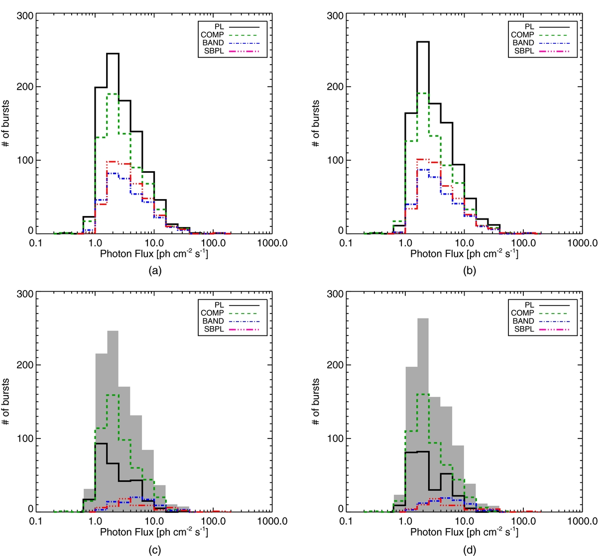
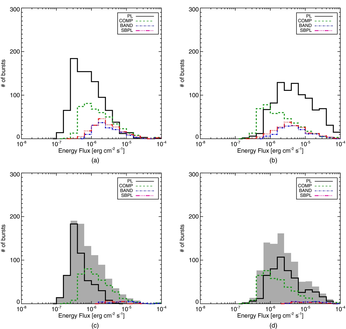
Standard image High-resolution imageThe distributions for the time-averaged energy flux and photon flux are shown in Figures 10 and 11, respectively. The photon and energy fluxes of the BEST sample have a median value of around 2.4 photons cm−2 s−1, and 3 × 10⁻⁷ erg cm−2 s−1, respectively in the 10–1000 keV band. When integrating over the full GBM spectral band, 10 keV–40 MeV, the BEST energy flux distribution broadens significantly, approximating a top hat function with a small high-flux tail spanning about two orders of magnitude. Note that the low-flux cutoff is due to both the sensitivity of the instrument and the clear deviation from a three-dimensional Euclidean distribution that is observed in a typical log N–log S plot (von Kienlin et al. 2014). In any case, the flux measurements with a more sensitive instrument will likely position the peak of the flux distribution at a lower flux value (see also Gruber et al. 2012). Similarly in Figures 12 and 13, the distributions for the BEST photon fluence and BEST energy fluence are depicted. The plots for the photon fluence appear to contain evidence of the duration bimodality of GRBs. While there is a discriminant peak at ∼30 photons cm−2 there is also a deviation from a log-normal distribution at smaller photon fluence values. Fitting the photon fluence distribution in the 10–1000 keV band with a sum of two log-normal functions, we find peak values of  and
and  , respectively. Similarly, the distribution of the energy fluence in the 10–1000 keV band can also be fit by the sum of two log-normal functions which result in peak values of
  and
and  , respectively. It is interesting to note that while the Comp model is largely unaffected by the change in energy band due to the exponential cutoff, the Pl model shifts to one order of magnitude higher energy fluence values, as it overestimates the flux at higher energies (see Figure 12(d)). The brightest GRB contained in this catalog based on time-averaged photon flux is GRB 120323.507 (Guiriec et al. 2013) with a flux of ∼115 photons s−1 cm−2 and the burst with the largest average energy flux is GRB 111222.619 with an energy flux of ∼1.5 × 10⁻⁵ erg s−1 cm−2. The burst with the highest energy fluence is GRB 090902.462 (Abdo et al. 2009) with an energy fluence of ∼2.8 × 10⁻⁴ erg cm−2 while the burst with the highest photon fluence is GRB 090618.353 with a photon fluence of >2300 photons cm−2.

Figure 10. Distributions of energy flux in the 10 keV–1 MeV (a) and 10 keV–40 MeV (b) band from the GOOD F spectral fits. Note that the plotted distributions contain the flux on two different timescales: 1024 ms (long GRBs) and 64 ms (short GRBs). The BEST parameter distribution for the energy flux in both energy ranges is shown in (c) and (d). The gray filled histogram shows the total distribution and the constituents are shown in colors.
Download figure:
Standard image High-resolution image
Figure 11. Distributions of photon flux in the 10 keV–1 MeV (a) and 10 keV–40 MeV (b) band from the GOOD F spectral fits. Note that the plotted distributions contain the flux on two different timescales: 1024 ms (long GRBs) and 64 ms (short GRBs). The BEST parameter distribution for the photon flux in both energy ranges is shown in (c) and (d). The gray filled histogram shows the total distribution and the constituents are shown in colors.
Download figure:
Standard image High-resolution image
Figure 12. Distributions of energy fluence in the 10 keV–1 MeV (a) and 10 keV–40 MeV (b) band from the GOOD F spectral fits. The BEST parameter distribution for the energy fluence in both energy ranges is shown in (c) and (d). The gray filled histogram shows the total distribution and the constituents are shown in colors.
Download figure:
Standard image High-resolution image
Figure 13. Distributions of photon fluence in the 10 keV–1 MeV (a) and 10 keV–40 MeV (b) band from the GOOD F spectral fits. The BEST parameter distribution for the energy fluence in both energy ranges is shown in (c) and (d). The gray filled histogram shows the total distribution and the constituents are shown in colors.
Download figure:
Standard image High-resolution imageIn Figure 14 we present the BEST rest-frame spectral parameters for Epeak, Eb, Eiso and Liso where the latter two have been determined in the rest-frame energy band between 1/(1 + z) keV and 10/(1 + z) MeV. Both,  and
and  peak at roughly 600 keV and, similarly to the distributions in the observer frame, cover just two orders of magnitude. The Eiso distribution peaks at ∼1053 erg and extends over more than three orders of magnitude. Liso, on the other hand, has a median of ∼1052 erg s−1 and covers three orders of magnitude.

Figure 14. (a)  distribution of the F spectra fits from the BEST sample for long and short GRBs (light gray and dark gray filled histogram, respectively). (b) Same as (a) but for
  . (c) and (d) Distribution of Eiso and Liso of the fluence spectral fits from the BEST sample in the rest-frame energy band 1/(1 + z) keV to 10/(1 + z) MeV.
Download figure:
Standard image High-resolution imageIn Figure 15 we show the evolution of the BEST spectral parameters, α, β and Epeak, with redshift. While both the high-energy index and Epeak do not show a clear dependence with redshift (see also Gruber et al. 2011a), the low-energy index of the long GRBs shows a trend to steeper, i.e., softer, values at higher redshifts (see also Geng & Huang 2013). However, a Spearman rank correlation analysis shows that this correlation is not significant (P = 0.15).

Figure 15. BEST spectral parameters as a function of the redshift of the F spectral fits for short (black triangles) and long (light-gray diamonds) GRBs.
Download figure:
Standard image High-resolution image6.1.1. The Break Scale Δ
In order to test the behavior of the break scale Δ of the Sbpl model, we re-fitted all GOOD Sbpl spectra obtained from the F spectral fits. Contrary to the initial fits, we vary the break scale, thus increasing the number of free model parameters. After the fit, we applied the same quality cuts to the resulting parameters as for the GOOD Sbpl sample with the additional requirement that σΔ/Δ ⩽ 0.4. Out of the initial 384 Sbpl fits only 36 fulfilled this newly added criterion, with the fit not able to constrain 5 free parameters for the bulk of the GOOD sample. As intuitively obvious, only the most fluent portion of the sample could be fitted with such a complex model (see Figure 16), but it should be noted that the GRBs for which the break scale could be constrained are not necessarily the GRBs for which this model was selected as BEST in Section 5.2. In Figure 17 we show the distribution of Δ. As can be seen Δ varies between 0.1 and 0.7 with an average value of 0.4 ± 0.2. It is instructive to investigate how the additional free fit parameter affects the results of the other model components. In Figure 18 we show the relations between fixed and varying Eb, low- and high-energy power-law indices. The low-energy power-law index seems to tend toward shallower values (particularly when the index is already shallow with the fixed Δ) when letting Δ vary freely. In fact, 13 (36%) low–energy power–law indices are not consistent within 1σ. The high-energy power-law index has a tendency to steepen and 11 (31%) indices are not consistent within the 1σ limit. With 8 (22%) 1σ outliers, the situation is similar for Eb. In general, Eb tends toward harder values when Δ is allowed to vary.

Figure 16. Distribution of the energy fluence in the 10 keV–1 MeV energy range for the GOOD Sbpl F spectral fits (black solid histogram) and the GOOD Sbpl fluence spectral fits with varying break scale Δ (red filled histogram).
Download figure:
Standard image High-resolution image
Figure 17. Distribution of the break scale Δ of the Sbpl F spectral fits.
Download figure:
Standard image High-resolution image
Figure 18. Comparison of Sbpl model parameters with Δ free to vary and fixed to 0.3. Values consistent within 1σ (blue triangles) and not consistent within 1σ (black diamonds) including a line of equality (red dashed line) are shown.
Download figure:
Standard image High-resolution image6.2. P Spectral Fits
Similarly to the F spectral fits, we are going to present the results of the P spectral fits in this section.
The P spectral distributions have been produced by fitting the GRB spectra over the 1024 ms and 64 ms peak-flux duration of long and short bursts respectively. Note that the results from both long and short bursts are included in the following figures. The low-energy indices from the P selections of the BEST sample, as shown in Figure 19(b), have a median value of about −1.3 and show a bimodal distribution. This is due to the fact that more GRBs of the P sample are best fit by the Pl because, due to less photon fluence accumulation, the S/N decreases. Twenty percent of the BEST low-energy indices show α > −2/3 and violate the synchrotron "line-of-death," while an additional 32% of the indices are α < −3/2 and violate the synchrotron cooling limit, both of which are significantly larger percentages than those from the F spectra. The high-energy indices in Figure 20 peak at about −2.2 and again have a long tail toward steeper indices. The number of unconstrained high-energy indices increases when compared to the F spectra, again likely due to the poorer statistics resulting from shorter integration times. As has been shown with the F spectral fits, the Pl index serves as an average between low- and high-energy indices for the Band and Sbpl functions.

Figure 19. Distribution of the low-energy indices obtained from the GOOD P spectral fits (a). The BEST parameter distribution (gray filled histogram) and its constituents for the low-energy index is shown in (b).
Download figure:
Standard image High-resolution image
Figure 20. Distribution of the high-energy indices obtained from the GOOD P spectral fits (a). The BEST parameter distribution (gray filled histogram) and its constituents for the high-energy index is shown in (b).
Download figure:
Standard image High-resolution imageShown in Figure 21 is the ΔS distribution for the P spectra. This distribution seems consistent with the BATSE results found previously (Preece et al. 2002; Kaneko et al. 2006), but suffers from a deficit in values compared to the F fits largely due to the inability of the data to sufficiently constrain the high-energy power-law index. The distribution peaks at ∼1.3 and has a median value of 1.64.

Figure 21. Distributions of ΔS, the difference between the low- and high-energy spectral indices (α − β) for the P spectral fits. The BEST (black solid line), the GOOD BAND power-law indices (blue dash-dotted line) and the GOOD Sbpl power-law indices (red dash-dot-dot-dotted line) for the F spectral fits are shown. The first bin contains values less than 0, indicating that the centroid value of α is steeper than the centroid value of β.
Download figure:
Standard image High-resolution imageIn Figures 22 and 23, we show the distributions for Eb and Epeak, respectively. As was evident from the F spectra, the Eb from the Sbpl fits appears to peak at 100 keV. The Epeak distribution for the BEST sample peaks around 260 keV and covers just over two orders of magnitude, which is consistent with previous findings (Preece et al. 1998b; Kaneko et al. 2006). It should be noted that the data over the short timescales in the P spectra do not often favor either the Band or the Sbpl model, resulting in large parameter errors.

Figure 22. Distribution of the Eb obtained from the GOOD P spectral fits (a). The BEST parameter distribution (gray filled histogram) and its constituents for Eb is shown in (b).
Download figure:
Standard image High-resolution image
Figure 23. Distribution of the Epeak obtained from the GOOD P spectral fits (a). The BEST parameter distribution (gray filled histogram) and its constituents for Epeak is shown in (b).
Download figure:
Standard image High-resolution imageEven though it is less obvious, Figure 24 shows a correlation between the Epeak and low-energy power-law index and its uncertainty which is similar to the F spectral fits.

Figure 24. Comparison of the low-energy index and Epeak for three models from the P spectral fits. This comparison reveals a correlation between the Epeak energy and the uncertainty on the low-energy index: generally a lower energy Epeak tends to result in a less constrained low-energy index.
Download figure:
Standard image High-resolution imageIn addition, we calculate and show the ΔEpeak statistic in Figure 25 and, as was the case with the F spectra, ∼46% of the Band and Comp Epeak values are found to be outside the combined errors. If the allowed error range is extended to 3σ then only 8% of the Epeak values are not consistent.

Figure 25. Distribution of the ΔEpeak statistic for the Comp and Band models from P spectral fits. A value less than 1 indicates the Epeak values are within errors, while a value larger than 1 indicates the Epeak values are not within errors.
Download figure:
Standard image High-resolution imageThe distributions for the peak energy flux and photon flux are shown in Figures 26 and 27, respectively. The photon flux of the BEST sample peaks around 4.5 photons cm−2 s−1, and the energy flux of the BEST sample peaks at 6.4 × 10⁻⁷ erg cm−2 s−1 in the 10–1000 keV band. When integrating over the full GBM spectral band, 10 keV-40 MeV, the dispersion in the energy flux increases and approximates a top hat function with a small high-flux tail spanning about two orders of magnitude. The brightest short GRB in terms of peak photon flux is GRB 120323.507 at >580 photons s−1 cm−2 while the most energetic short GRB is GRB 090227.772 with an energy flux of ∼8.3 × 10⁻⁵ erg s−1 cm−2.

Figure 26. Distributions of energy flux in the 10 keV–1 MeV (a) and 10 keV–40 MeV (b) band from the GOOD P spectral fits. Note that the plotted distributions contain the flux on two different timescales: 1024 ms (long GRBs) and 64 ms (short GRBs). The BEST parameter distribution for the energy flux in both energy ranges is shown in (c) and (d). The gray filled histogram shows the total distribution and the constituents are shown in colors.
Download figure:
Standard image High-resolution image
Figure 27. Distributions of photon flux in the 10 keV–1 MeV (a) and 10 keV–40 MeV (b) band from the GOOD P spectral fits. Note that the plotted distributions contain the flux on two different timescales: 1024 ms (long GRBs) and 64 ms (short GRBs). The BEST parameter distribution for the photon flux in both energy ranges is shown in (c) and (d). The gray filled histogram shows the total distribution and the constituents are shown in colors.
Download figure:
Standard image High-resolution imageIn Figure 28 we present the rest-frame spectral parameters for Epeak, Eb, Eiso and Liso of the P spectral fits where the latter two have been determined in the rest-frame energy band between 1/(1 + z) keV and 10/(1 + z) MeV. Both,  and
and  peak at roughly 600 keV and, similarly to the distributions in the observer frame, cover just two orders of magnitude. The Eiso distribution is narrower than the one obtained from the F spectral fits and has a median of ∼1052 erg. Liso, on the other hand, has a median of ∼3 × 1052 erg s−1 and covers ∼3 orders of magnitude.

Figure 28. (a)  distribution of the P spectra fits from the BEST sample for long and short GRBs (light gray and dark gray filled histogram, respectively). (b) Same as (a) but for
  . (c) and (d) Distribution of Eiso and Liso of the fluence spectral fits from the BEST sample in the rest-frame energy band 1/(1 + z) keV to 10/(1 + z) MeV.
Download figure:
Standard image High-resolution imageIn Figure 29 we show the evolution of the BEST spectral parameters, α, β and Epeak, with redshift. None of the parameters shows a dependence with redshift.

Figure 29. BEST spectral parameters as a function of the redshift of the P spectral fits for short (black triangles) and long (light-gray diamonds) GRBs.
Download figure:
Standard image High-resolution image6.3. Comparing the F with the P Spectral Fits
When studying the two types of spectra in this catalog, it is instructive to study the similarities and differences between the resulting parameters (see Table 3). Plotted in Figure 30 are the low-energy indices, high-energy indices, and Epeak energies of the P spectra as a function of the corresponding parameters from the F spectra. Most of the P spectral parameters correlate with the F spectral parameters on the order of unity. There are particular regions in each plot where outliers exist, and these areas indicate that either the GRB spectrum is poorly sampled or that significant spectral evolution exists in the F measurement of the spectrum that skews the time-integrated spectral values. Examples of the former case are when the low-energy index is ≳ − 1.2 or the high-energy index is steeper than average (≲ − 2).

Figure 30. P spectral parameters as a function of the fluence spectral parameters for the GOOD sample. For all three parameters there is evidence for a strong correlation between the parameters found for the F spectra and those for the P spectra. Note that the Pl index is shown in both (a) and (b) for comparison.
Download figure:
Standard image High-resolution imageTable 3. The Median Parameter Values and the 68% CL of the Distributions of the GOOD Sample
| Model | Low-energy | High-energy | Epeak | Ebreak | Photon Flux | Energy Flux | ΔS |
|---|---|---|---|---|---|---|---|
| Index | Index | (keV) | (keV) | (photons s−1 cm−2) | (10−7 erg s−1 cm−2) | ||
| Fluence spectra | |||||||
| Pl |  |
⋅⋅⋅ | ⋅⋅⋅ | ⋅⋅⋅ |  |
 |
⋅⋅⋅ |
| Comp |  |
⋅⋅⋅ |  |
⋅⋅⋅ |  |
 |
⋅⋅⋅ |
| Sbpl |  |
 |
 |
 |
 |
 |
 |
| Band |  |
 |
 |
 |
 |
 |
 |
| BEST |  |
 |
 |
 |
 |
 |
 |
| Peak flux spectra | |||||||
| Pl |  |
⋅⋅⋅ | ⋅⋅⋅ | ⋅⋅⋅ |  |
 |
⋅⋅⋅ |
| Comp |  |
⋅⋅⋅ |  |
⋅⋅⋅ |  |
 |
⋅⋅⋅ |
| Sbpl |  |
 |
 |
 |
 |
 |
 |
| Band |  |
 |
 |
 |
 |
 |
 |
| BEST |  |
 |
 |
 |
 |
 |
 |
Download table as: ASCIITypeset image
It is common belief that Epeak is significantly larger at the peak of the GRB, compared to the average Epeak. Figure 30(c), and similar results found in Goldstein et al. (2012) and Nava et al. (2011), seems to contradict this belief with marginal difference between Epeak measured at the peak of the photon flux and Epeak measured over the full duration of the burst.
However, time-resolved spectral analyses in the past have shown (e.g., Kaneko et al. 2006; Lu et al. 2012 for BATSE and GBM GRBs, respectively) that two different Epeak-evolution patterns can (co-)exist in a single GRB:
- 1.Epeak can evolve from hard-to-soft and/or
- 2.Epeak shows a tracking behavior with respect to the photon flux.
If a GRB evolves from hard-to-soft, the peak of the photon flux does not necessarily correspond to the highest Epeak value (see also Crider et al. 1999). Only when Epeak tracks the intensity its highest value is indeed expected at the peak photon flux.
In addition, the time-averaged Epeak is also dependent on the ratio of the peak photon flux versus the average photon flux of the GRB. A larger ratio, i.e., a higher photon flux at the peak of the burst, skews the average Epeak toward the Epeak found at peak flux. Therefore, a marginal difference between Epeak of the F spectral fits and P spectral is expected.
In a forthcoming catalog (H. F. Yu et al., in preparation), the results of a time-resolved study of GBM GRBs will be presented.
To aid in the study of the systematics of the parameter estimation, as well as the effect of statistics on the fitting process, we investigate the behavior parameter values as a function of accumulation time and the photon fluence for the F BEST spectra and peak photon flux for the P BEST spectra, respectively. These distributions are shown in Figures 31–33, respectively. As the photon fluence is correlated with the duration of a burst (see again Figure 1(b)) any correlation of a spectral parameter with the accumulation time will also be correlated with photon fluence.
When fitting the time-integrated spectrum of a burst, we find the low- and high-energy indices trend toward steeper values for bursts with longer accumulation times. The simple Pl index trends from shallow values of ∼ − 1.3 to a steeper value of ∼ − 2. The low-energy index for a spectrum with curvature tends to exhibit an unusually shallow value of ∼ − 0.4 for short GRBs or extremely low fluence spectra, and steepens to ∼ − 1.5 for longer GRBs or higher fluence spectra. Similarly, the high-energy index trends from ∼ − 1.2 at short durations or low fluence to ∼ − 2.7 at long durations or high fluence, although this is complicated by unusually steep and poorly constrained indices that indicate that an exponential cutoff may result in a more reliable spectral fit. When inspecting the Epeak as a function of accumulation time the resulting plot is reminiscent of the hardness/duration correlation with two distinct regions for the long and short GRBs. As for the correlation between Epeak and photon fluence a trend is much less apparent. If a burst is assumed to have significant spectral evolution, then obviously the Epeak will change values through the time history of the burst, typically following the traditional hard-to-soft energy evolution. For this reason, spectra that integrate over increasingly more time will tend to suppress the highest energy of Epeak within the burst, so a general decrease in Epeak is expected with longer integration times. However, the photon fluence convolves the integration time with the photon flux. This means that an intense burst with a short duration and high Epeak may have on the order the same fluence as a much longer but less intense burst with a smaller Epeak. This causes significant broadening to the decreasing trend as shown in Figure 32(c).
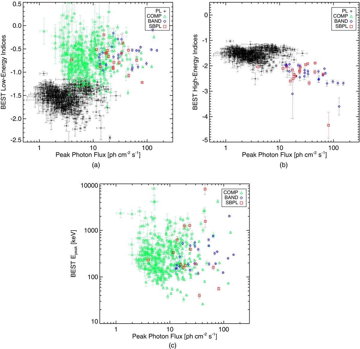
The distribution of parameters as a function of the peak photon flux, however, is much less clear. The distributions shown in Figure 33 are more susceptible to uncertainty because of smaller statistics involved in the study of the P section of the GRB, except in some cases where the peak photon flux is on the order of the photon fluence. Ignoring the regions where the parameters are poorly constrained, another trend emerges from the low-energy indices; they appear to become slightly more shallow as the photon flux increases. The high-energy indices, however, appear to be unaffected by the photon flux, although a trend of steeper indices with higher photon fluxes seems apparent. Finally, no obvious trend is visible for Epeak as a function of the peak photon flux (Spearman rank correlation coefficient of −0.05 with a chance probability of P = 0.9). However, when inspecting Epeak as a function of peak energy flux, as shown in Figure 34, a correlation becomes apparent (Spearman rank correlation coefficient of ∼1 with P = 8 × 10−08). The lack and existence of a correlation between Epeak and the photon and energy flux, respectively is expected because it is the energy of collected photons and not their number that drives the hardness (and thus Epeak) of a GRB.
The spectral results, including the best fit spectral parameters and the photon model, are stored in files following the FITS standard and will be hosted as a public data archive on High-Energy Astrophysics Science Archive Research Center (HEASARC).16 The values returned by default in a Browse search of the catalog are the most recent values, which will be the results presented here upon acceptance of this paper. However, the values and results obtained by Goldstein et al. (2012) will still be available by ftp. The keyword scatalog indicates which catalog a file belongs to. Both the differences between the methodologies and how to retrieve the older files will be fully documented at HEASARC.
7. SUMMARY AND DISCUSSION
After four successful years, GBM continues to be a prime instrument for GRB observations. The second GBM spectral catalog includes 943 GRBs detected by GBM during 4 yr of operation. We presented the spectral properties of these bursts both from a time-integrated, and a peak-flux analysis. Four photon model fits were applied to each selection, resulting in more than 7500 spectral fits. We have described subsets of the full results in the form of data cuts based on parameter uncertainty, as well as employing model comparison techniques to select the most statistically preferred model for each GRB. The analysis of each GRB was performed as objectively as possible, in an attempt to minimize biased systematic errors inherent in subjective analysis. The methods we have described treat all bursts equally, and we have presented the ensemble of observed spectral properties of GBM GRBs.
Although most of the resulting parameter distributions are similar to the ones found by other GRB missions, some contain important differences. For example, thanks to the two BGO detectors, burst data extend into the high-energy domain which, in the past, has been accessible only by the Solar Maximum Mission Gamma Ray Spectrometer (Harris & Share 1998) and the PHEBUS instrument onboard the Granat spacecraft (Barat et al. 2006). While there does not seem to be a new population of bursts with high Epeak values in their time-integrated spectra, 40 GRBs of the BEST fluence spectra and 37 of the BEST P spectrum have Epeak values above 1 MeV. In order to verify whether the lack of GRBs with high Epeak values in their time-integrated spectra is intrinsic or an instrumental bias (decreasing effective are in the BGOs) requires simulations which go beyond the scope of this catalog. We emphasize that there are indeed GRBs with very high Epeak values in their time-resolved spectra, such as, e.g., GRB 110721A (Axelsson et al. 2012) which has the highest observer-frame Epeak value (15 ± 2 MeV) known to date. In a forthcoming catalog of time-resolved spectra of GBM GRBs (H. F. Yu et al., in preparation) this will be investigated in more detail.
Another interesting result of the parameter distributions is the ΔS parameter, the difference between the low- and high-energy spectral indices. This is an important quantity because current models for the GRB prompt emission mechanism can be broken into two categories: magnetic (e.g., Lee et al. 2000) or driven by internal/external shocks (e.g., Rees & Meszaros 1992). Thus, by comparing ΔS to the predictions by the SSM, it is possible to obtain useful insights into the emission mechanisms of GRBs. As our results for the ΔS distribution are compatible and in line with the results obtained by Preece et al. (2002) and Kaneko et al. (2006) it can concluded that the predictions of the SSM model, in its simplest form, are not reconcilable neither with the observations made by BATSE nor those performed by GBM.
Thanks to the rapid localizations of the Swift satellite, necessary to identify a redshift for any given burst, and the broad coverage of the GBM we could study many spectral properties in the rest frame of the GRB. This results in the largest  , Eiso and Liso sample to date which have been analyzed coherently and consistently with an unified methodology, thus minimizing systematic effects. This may be helpful in assessing whether or not well known correlations in the GRB literature are indeed real or due to statistical fluctuations and systematical issues.
The differences between various GBM spectral catalogs (e.g., Nava et al. 2011) were extensively discussed in Goldstein et al. (2012). Small discrepancies between Goldstein et al. (2012)'s first GBM spectral catalog and the one presented here (e.g., different BEST models for the same GRB, fraction of bursts best fit with a given model) are mainly due to enhanced and modified criteria in determining the BEST and GOOD sample, updated analysis software and response matrices and the usage of different statistical criteria, i.e., C-Stat instead of χ2 to determine the preferred model. These differences, see also Table 4, are representative of divergent methodologies and samples; therefore the reader should take care to understand how the values in the catalogs are derived. Certainly, there are avenues of investigation that require more detailed work and analysis or perhaps a different methodology. This catalog should be treated as a starting point for future research on interesting bursts and ideas. As has been the case in previous GRB spectral catalogs, we hope this catalog will be of great assistance and importance to the search for the physical properties of GRBs and other related studies.

Figure 31. BEST spectral parameters as a function of the accumulation time for F spectral fits. Note that the Pl index is shown in both (a) and (b) for comparison.
Download figure:
Standard image High-resolution image
Figure 32. BEST spectral parameters as a function of the model photon fluence of the F spectral fits. Note that the Pl index is shown in both (a) and (b) for comparison.
Download figure:
Standard image High-resolution image
Figure 33. BEST spectral parameters as a function of the model peak photon flux of the P spectral fits. Note that the Pl index is shown in both (a) and (b) for comparison.
Download figure:
Standard image High-resolution image
Figure 34. BEST Epeak as a function of the model energy flux of the P spectral fits.
Download figure:
Standard image High-resolution image
Table 4. The Median Parameter Values and the 68% CL of the BEST Model Fits
| Data Set | Low-energy | High-energy | Epeak | Ebreak | Photon Flux | Energy Flux |
|---|---|---|---|---|---|---|
| Index | Index | (keV) | (keV) | (photons s−1 cm−2) | (10−7 erg s−1 cm−2) | |
| Fluence | ||||||
| This Catalog BEST |  |
 |
 |
 |
 |
 |
| Goldstein et al. (2012) |  |
 |
 |
 |
 |
 |
| Nava et al. (2011) |  |
 |
 |
⋅⋅⋅ | ⋅⋅⋅ |  |
| Kaneko et al. (2006) |  |
 |
 |
 |
⋅⋅⋅ | ⋅⋅⋅ |
| Peak flux spectra | ||||||
| This Catalog BEST |  |
 |
 |
 |
 |
 |
| Goldstein et al. (2012) |  |
 |
 |
 |
 |
 |
| Nava et al. (2011) |  a a |
 |
 |
⋅⋅⋅ | ⋅⋅⋅ |  |
| Kaneko et al. (2006) |  |
 |
 |
 |
⋅⋅⋅ | ⋅⋅⋅ |
Note.
a ow-energy index of the peak-flux spectra with curved function only.
Download table as: ASCIITypeset image
We thank the reviewer for his/her comments, which significantly contributed to improving the quality of the publication. The GBM project is supported by the German Bundesministeriums für Wirtschaft und Technologie (BMWi) via the Deutsches Zentrum für Luft und Raumfahrt (DLR) under the contract numbers 50 QV 0301 and 50 OG 0502.
Footnotes
- 14
Formerly known as the Gamma-Ray Large Area Space Telescope or GLAST.
- 15
- 16