


ABSTRACT
We present the first results from our high-precision infrared (IR) astrometry program at the Canada–France–Hawaii Telescope. We measure parallaxes for 83 ultracool dwarfs (spectral types M6–T9) in 49 systems, with a median uncertainty of 1.1 mas (2.3%) and as good as 0.7 mas (0.8%). We provide the first parallaxes for 48 objects in 29 systems, and for another 27 objects in 17 systems, we significantly improve upon published results, with a median (best) improvement of 1.7 times (5 times). Three systems show astrometric perturbations indicative of orbital motion; two are known binaries (2MASS J0518−2828AB and 2MASS J1404−3159AB) and one is spectrally peculiar (SDSS J0805+4812). In addition, we present here a large set of Keck adaptive optics imaging that more than triples the number of binaries with L6–T5 components that have both multi-band photometry and distances. Our data enable an unprecedented look at the photometric properties of brown dwarfs as they cool through the L/T transition. Going from ≈L8 to ≈T4.5, flux in the Y and J bands increases by ≈0.7 mag and ≈0.5 mag, respectively (the Y- and J-band "bumps"), while flux in the H, K, and L' bands declines monotonically. This wavelength dependence is consistent with cloud clearing over a narrow range of temperature, since condensate opacity is expected to dominate at 1.0–1.3 μm. Interestingly, despite more than doubling the near-IR census of L/T transition objects, we find a conspicuous paucity of objects on the color–magnitude diagram just blueward of the late-L/early-T sequence. This "L/T gap" occurs at (J − H)MKO = 0.1–0.3 mag, (J − K)MKO = 0.0–0.4 mag, and implies that the last phases of cloud evolution occur rapidly. Finally, we provide a comprehensive update to the absolute magnitudes of ultracool dwarfs as a function of spectral type using a combined sample of 314 objects.
Export citation and abstract BibTeX RIS
1. INTRODUCTION
Few astronomical measurements are as direct and model-independent as trigonometric parallaxes, as they rely solely on geometry and an accurate ephemeris of Earth's orbit. Distances determined by parallaxes form the foundation of much of modern astrophysics, e.g., enabling the creation of the Hertzsprung–Russell diagram and establishing a key rung in the cosmological distance ladder. Since the first stellar parallax measurement (61 Cyg; Bessel 1838), astrometry programs have continuously evolved using new technology to achieve ever-expanding science objectives. Photographic plates dominated parallax work for many decades, but the need to reach fainter stars eventually required the use of CCDs with their low noise, high quantum efficiency, and capacity for large dynamic range. Pioneering work in this area demonstrated that precise astrometry was in fact possible with such devices (e.g., see Monet & Dahn 1983) even though the field of view of early detectors was small by today's standards. As CCDs have grown in size they have become the dominant tool for high-precision astrometry. With the advent of large-format infrared (IR) arrays it is now possible to extend parallax measurements to large samples of the coldest known objects outside the solar system: brown dwarfs.
Over the past decade, several ground-based astrometry programs have laid the foundation for understanding the basic evolution of brown dwarfs on the color–magnitude diagram (CMD). Infrared parallax programs account for about two thirds of parallaxes for brown dwarfs with spectral types ⩾L4 (e.g., Tinney et al. 2003; Vrba et al. 2004; Marocco et al. 2010), with red optical programs providing the remaining one third, mostly at earlier types (e.g., Dahn et al. 2002; Schilbach et al. 2009; Andrei et al. 2011). Companions to stars with Hipparcos parallaxes also make up a significant fraction of the current sample of ⩾L4 dwarfs with parallaxes, roughly half as many as have been measured directly in infrared astrometry programs. Parallax measurements for very low mass stars and brown dwarfs of earlier spectral types (M6–L4) are dominated by red optical astrometry programs at the USNO (Monet et al. 1992; Dahn et al. 2002) and elsewhere (e.g., Tinney et al. 1995; Tinney 1996; Costa et al. 2006; Gatewood & Coban 2009; Lépine et al. 2009; Schilbach et al. 2009; Andrei et al. 2011).
There is a pressing demand for the highest possible precision in ultracool dwarf distance measurements. This is because dynamical mass studies are now providing the strongest tests of substellar models (e.g., Bouy et al. 2004; Liu et al. 2008; Dupuy et al. 2009b, 2009c, 2010; Konopacky et al. 2010), and precise parallaxes are crucial for such work. Dynamical mass uncertainties from visual binary orbits are almost always dominated by the error in the distance since mass ∝d3. Thus, to achieve a 10% mass uncertainty requires parallax errors of ≈3%. Among ground-based measurements for ⩾L4 dwarfs such precision is not common (only 26% of parallaxes) and has previously been achieved only for relatively nearby objects (⩽13 pc).
Furthermore, despite the past successes of the parallax programs described above, there are still important aspects of brown dwarf evolution that would benefit from a larger set of distance measurements: young field brown dwarfs (e.g., Kirkpatrick et al. 2006; Allers et al. 2009; Cruz et al. 2009), the coldest brown dwarfs (≲500 K, e.g., Lucas et al. 2010; Cushing et al. 2011), and the L/T transition (e.g., Liu et al. 2006; Saumon & Marley 2008). Samples pertaining to the first two subjects have only recently begun to be uncovered, and parallax measurements are underway by multiple groups for both young field dwarfs (e.g., Teixeira et al. 2008; M. C. Liu et al., submitted) and the latest type T dwarfs (e.g., Smart et al. 2010; Liu et al. 2011b). In contrast, objects with properties intermediate between red L dwarfs and blue T dwarfs have been known since some of the earliest surveys to yield brown dwarfs (Leggett et al. 2000; Geballe et al. 2002). However, to date, only six single objects in this range (L9–T4) have parallaxes, compared to 33 parallaxes for single T4.5–T9 dwarfs and 29 parallaxes for single L4–L8.5 dwarfs. (There are an additional ≈4 components of binaries in the L9–T4 range with parallaxes, but this exact number is subject to the somewhat uncertain spectral classification of most of these components.) There is a present deficiency in the number of L/T transition objects with parallaxes and thus in our ability to characterize one of the most important phases of brown dwarf evolution.
To address the need for high-precision parallaxes of ultracool binaries, we initiated an infrared parallax program at the Canada–France–Hawaii Telescope (CFHT) in 2007. We concentrated our observations on a sample of ultracool binaries with a wide range of component spectral types (M6–T9) that includes all systems observable with CFHT that are likely to yield dynamical masses in the next ≈decade. This dynamical mass sample also forms the basis of our ongoing Keck adaptive optics (AO) orbital monitoring program, which to date has tripled the number of ultracool binaries with dynamical masses sufficiently precise for model testing (see Dupuy et al. 2011, and references therein). The primary goals of this first phase of our CFHT program are to expand the sample of dynamical mass measurements for brown dwarfs and enable more precise masses from the existing sample of orbits by reducing distance errors. In addition to the dynamical mass sample, we included in our original parallax program several other binaries that are not necessarily amenable to orbit determination in the near future but that have components bridging the L/T transition. This L/T sample is motivated by the deficit of parallaxes for objects with spectral types L9–T4 and by the inherent utility of binaries for substellar model tests given their identical age and composition (e.g., Liu & Leggett 2005; Liu et al. 2010). This supplemental sample of L/T binaries provides the context needed for comparisons to the field population as our orbital monitoring program yields dynamical mass measurements for L/T transition objects (e.g., Dupuy et al. 2009c). Finally, we have also been targeting binaries with the coldest known components (≳T8), and this has resulted in a parallax for CFBDS J1458+1013AB, which has component types of T9 and >T10 (Liu et al. 2011b, updated parallax given in this paper).
We present here the first large set of results of our CFHT infrared parallax program along with a complete description of our astrometric methods (Section 2). This sample includes 34 binaries and 15 single objects that have been chosen because they will be useful for measuring dynamical masses in the future, studying the L/T transition, and increasing the number of parallaxes for mid- to late-T dwarfs. We also present supporting observations from other telescopes, including a large collection of resolved photometry for tight binaries from Keck, the Hubble Space Telescope (HST), and the Very Large Telescope (VLT; Section 3) and integrated-light near-infrared spectroscopy (Section 4). The ensemble of these new measurements provides an unprecedented view of the L/T transition.
2. CFHT/WIRCam ASTROMETRIC MONITORING
Since 2007, we have been using the facility near-IR camera WIRCam at CFHT to conduct an astrometric monitoring program with the goal of measuring parallaxes for ultracool dwarfs. WIRCam comprises a mosaic of four 2048×2048 Hawaii-2RG infrared arrays, each with a field of view of 10 4 × 10⁴ and pixel scale of 0
 3 pixel−1 (Puget et al. 2004). At each epoch, we obtained ≈20–30 dithered images of our targets, which were always centered on the northeast array of WIRCam. All images were first processed at CFHT using the WIRCam pipeline 'I'iwi, which performs a nonlinearity correction, dark subtraction, flat fielding, bad pixel masking, sky subtraction, and cross-talk removal for each image.4 We obtained data in the J band for most targets, as this filter afforded the lowest sky background and thus the most reference stars. Targets brighter than J < 13.3 mag were at risk of saturating in the 5 s minimum integration time of WIRCam, so for these targets we used the narrow K-band filter (KH2) centered at 2.122 μm with a bandwidth of 0.032 μm (1.5%). Table 1 summarizes our target list and the details of our observations.
Table 1. CFHT/WIRCam Parallax Observations
| Target | Spec. Type | CFHT | FWHM | Max(ΔAM) | Nfr | Nep | Δt | Nref | Ncal | πabs − πrel |
|---|---|---|---|---|---|---|---|---|---|---|
| Optical/IR | Filter | ('') | (yr) | (mas) | ||||||
| SDSS J000013.54+255418.6 | .../T4.5 | J | 0.58 ± 0.07 | 0.014 | 291 | 12 | 2.43 | 124 | 114 | 1.31 ± 0.11 |
| 2MASSI J0003422−282241 | M7.5/... | KH2 | 0.59 ± 0.14 | 0.031 | 213 | 11 | 2.32 | 21 | 17 | 2.07 ± 0.59 |
| LP 349-25AB | M8/M8 | KH2 | 0.62 ± 0.09 | 0.062 | 456 | 15 | 2.96 | 33 | 30 | 1.74 ± 0.31 |
| ULAS J003402.77−005206.7 | .../T8.5 | J | 0.57 ± 0.09 | 0.018 | 66 | 9 | 2.18 | 73 | 64 | 1.46 ± 0.18 |
| 2MASS J00501994−3322402 | .../T7 | J | 0.82 ± 0.14 | 0.023 | 137 | 7 | 2.19 | 77 | 37 | 1.56 ± 0.25 |
| CFBDS J005910.90−011401.3 | .../T8.5 | J | 0.63 ± 0.15 | 0.021 | 71 | 8 | 2.14 | 88 | 53 | 1.37 ± 0.17 |
| 2MASSI J0415195−093506 | T8/T8 | J | 0.70 ± 0.08 | 0.026 | 136 | 8 | 2.28 | 124 | 44 | 1.38 ± 0.19 |
| SDSSp J042348.57−041403.5AB | L7.5/T0 | J | 0.72 ± 0.15 | 0.027 | 100 | 11 | 4.27 | 128 | 63 | 1.41 ± 0.17 |
| 2MASS J05185995−2828372AB | L7/T1p | J | 0.73 ± 0.13 | 0.022 | 131 | 12 | 4.20 | 182 | 59 | 1.24 ± 0.16 |
| 2MASSI J0559191−140448 | T5/T4.5 | J | 0.77 ± 0.07 | 0.006 | 139 | 6 | 1.83 | 225 | 101 | 0.85 ± 0.09 |
| 2MASS J07003664+3157266AB | L3.5/... | KH2 | 0.61 ± 0.11 | 0.068 | 216 | 12 | 4.12 | 94 | 86 | 1.19 ± 0.15 |
| LHS 1901AB | M7/M7 | KH2 | 0.67 ± 0.11 | 0.054 | 225 | 16 | 3.81 | 73 | 70 | 1.50 ± 0.20 |
| 2MASSI J0727182+171001 | T8/T7 | J | 0.66 ± 0.17 | 0.036 | 268 | 12 | 2.46 | 331 | 106 | 0.90 ± 0.08 |
| 2MASSI J0746425+200032AB | L0.5/L1 | KH2 | 0.65 ± 0.09 | 0.031 | 259 | 10 | 3.86 | 55 | 54 | 1.42 ± 0.21 |
| SDSS J080531.84+481233.0 | L4/L9.5 | J | 0.70 ± 0.16 | 0.046 | 237 | 13 | 4.03 | 72 | 70 | 1.43 ± 0.17 |
| 2MASSs J0850359+105716AB | L6/... | J | 0.61 ± 0.13 | 0.021 | 89 | 9 | 4.16 | 182 | 174 | 1.16 ± 0.11 |
| 2MASSI J0856479+223518AB | L3:/... | J | 0.68 ± 0.15 | 0.007 | 64 | 8 | 2.41 | 115 | 113 | 1.44 ± 0.13 |
| 2MASSW J0920122+351742AB | L6.5/T0p | J | 0.64 ± 0.15 | 0.016 | 172 | 15 | 4.35 | 77 | 68 | 1.56 ± 0.17 |
| SDSS J092615.38+584720.9AB | .../T4.5 | J | 0.62 ± 0.05 | 0.010 | 198 | 11 | 4.12 | 73 | 70 | 1.38 ± 0.15 |
| 2MASSI J1017075+130839AB | L2:/L1 | J | 0.67 ± 0.12 | 0.013 | 303 | 13 | 4.12 | 35 | 34 | 1.69 ± 0.27 |
| SDSS J102109.69−030420.1AB | T3.5/T3 | J | 0.75 ± 0.08 | 0.012 | 193 | 9 | 3.09 | 69 | 64 | 1.34 ± 0.15 |
| SDSS J111010.01+011613.1 | .../T5.5 | J | 0.66 ± 0.15 | 0.006 | 102 | 10 | 3.15 | 80 | 74 | 1.56 ± 0.17 |
| 2MASS J11145133−2618235 | .../T7.5 | J | 0.57 ± 0.10 | 0.058 | 131 | 7 | 2.02 | 61 | 21 | 0.97 ± 0.27 |
| LHS 2397aAB | M8/... | KH2 | 0.63 ± 0.11 | 0.454 | 201 | 13 | 3.22 | 30 | 28 | 1.76 ± 0.32 |
| 2MASSW J1146345+223053AB | L3/... | J | 0.60 ± 0.08 | 0.013 | 173 | 7 | 2.26 | 38 | 35 | 1.84 ± 0.30 |
| 2MASS J12095613−1004008AB | T3.5/T3 | J | 0.55 ± 0.11 | 0.019 | 215 | 12 | 3.92 | 28 | 16 | 1.31 ± 0.32 |
| DENIS-P J1228.2−1547AB | L5/L6:: | J | 0.66 ± 0.14 | 0.030 | 125 | 11 | 2.26 | 102 | 44 | 1.35 ± 0.19 |
| 2MASSW J1239272+551537AB | L5/... | J | 0.66 ± 0.09 | 0.015 | 226 | 9 | 2.26 | 38 | 33 | 1.70 ± 0.31 |
| Kelu-1ABa | L2/... | J | 0.75 ± 0.11 | 0.012 | 211 | 9 | 2.26 | 98 | 39 | 1.12 ± 0.20 |
| ULAS J133553.45+113005.2 | .../T8.5 | J | 0.63 ± 0.15 | 0.025 | 118 | 10 | 1.95 | 175 | 162 | 1.00 ± 0.09 |
| 2MASS J14044948−3159330AB | T0/T2.5 | J | 0.63 ± 0.13 | 0.030 | 214 | 11 | 2.25 | 276 | 80 | 0.81 ± 0.10 |
| SDSS J141624.08+134826.7 | L6/L6p:: | KH2 | 0.62 ± 0.08 | 0.149 | 246 | 13 | 1.95 | 22 | 19 | 2.12 ± 0.60 |
| CFBDS J145829+10134AB | .../T9.5 | J | 0.66 ± 0.18 | 0.022 | 119 | 11 | 1.96 | 324 | 262 | 0.89 ± 0.06 |
| 2MASSW J1503196+252519 | T6/T5 | J | 0.60 ± 0.09 | 0.004 | 98 | 7 | 2.00 | 58 | 53 | 1.34 ± 0.19 |
| SDSS J150411.63+102718.3 | .../T7 | J | 0.62 ± 0.09 | 0.058 | 63 | 6 | 1.94 | 102 | 91 | 1.20 ± 0.14 |
| SDSS J153417.05+161546.1AB | .../T3.5 | J | 0.60 ± 0.11 | 0.014 | 219 | 11 | 2.35 | 139 | 132 | 1.10 ± 0.11 |
| 2MASSI J1534498−295227AB | T6/T5.5 | J | 0.61 ± 0.12 | 0.019 | 241 | 16 | 2.36 | 475 | 170 | 0.60 ± 0.06 |
| 2MASSW J1553022+153236ABa | .../T7 | J | 0.86 ± 0.05 | 0.018 | 119 | 8 | 2.18 | 145 | 137 | 0.95 ± 0.09 |
| SDSS J162838.77+230821.1 | .../T7 | J | 0.57 ± 0.12 | 0.030 | 110 | 9 | 2.32 | 166 | 155 | 1.02 ± 0.09 |
| 2MASSW J1728114+394859AB | L7/... | J | 0.56 ± 0.15 | 0.021 | 197 | 11 | 3.32 | 251 | 45 | 0.97 ± 0.15 |
| LSPM J1735+2634AB | M7.5/... | KH2 | 0.54 ± 0.11 | 0.029 | 199 | 9 | 3.24 | 90 | 76 | 1.28 ± 0.17 |
| 2MASSW J1750129+442404AB | M7.5/M8 | KH2 | 0.57 ± 0.11 | 0.029 | 239 | 13 | 2.18 | 64 | 61 | 1.41 ± 0.19 |
| 2MASSI J1847034+552243AB | M6.5/... | KH2 | 0.58 ± 0.09 | 0.020 | 291 | 13 | 2.90 | 99 | 88 | 1.26 ± 0.14 |
| SDSS J205235.31−160929.8AB | .../T1: | J | 0.65 ± 0.15 | 0.022 | 422 | 17 | 2.22 | 243 | 59 | 0.88 ± 0.13 |
| 2MASSI J2132114+134158AB | L6/... | J | 0.57 ± 0.16 | 0.018 | 616 | 24 | 2.92 | 328 | 77 | 0.94 ± 0.11 |
| 2MASSW J2140293+162518AB | M8.5/... | KH2 | 0.55 ± 0.10 | 0.007 | 275 | 14 | 2.90 | 81 | 75 | 1.31 ± 0.15 |
| 2MASSW J2206228−204705AB | M8/M8 | KH2 | 0.58 ± 0.07 | 0.025 | 291 | 18 | 2.34 | 32 | 29 | 1.92 ± 0.39 |
| 2MASSW J2224438−015852 | L4.5/L3.5 | J | 0.65 ± 0.16 | 0.019 | 357 | 19 | 3.22 | 121 | 33 | 1.34 ± 0.24 |
| DENIS-P J225210.73−173013.4AB | .../L7.5 | J | 0.66 ± 0.22 | 0.021 | 411 | 16 | 2.21 | 72 | 28 | 1.59 ± 0.32 |
Notes. Opt./IR Spec. Type: for targets that are binaries, the integrated-light spectral type is listed. Spectrally peculiar objects are denoted by "p" and types uncertain by ±1 and ±2 are denoted by ":" and "::," respectively. FWHM: the median and rms of the FWHM as measured from the science target. ΔAMmax: maximum difference in airmass over all epochs. Nep: number of distinct observing epochs (i.e., nights). Nfr: total number of frames obtained (typically 20–30 per epoch). Nref: number of reference stars used. Ncal: subset of reference stars used in the absolute astrometric calibration (i.e., those available in SDSS, 2MASS, or USNO-B). πabs − πrel: offset from relative to absolute parallax computed for each field using the Besançon model of the Galaxy (Robin et al. 2003) as described in Section 2.4.2.
aKelu-1AB and 2MASS J1553+1532AB are extended in our CFHT imaging, which resulted in somewhat larger FWHM than for other targets observed at similar airmass. This is consistent with the fact that these are both wide, ≈03 binaries (Liu & Leggett 2005; Burgasser et al. 2006c).
Download table as: ASCIITypeset image
The CFHT data presented herein were mostly collected from the fall semester of 2007 to spring 2010, with 89 hr of queue-scheduled CFHT time allocated over six semesters. We have continued monitoring some targets in later semesters to improve their parallax errors, and the most recent data presented here come from early 2012. The median seeing for all the CFHT data presented here is 063, as judged by the target FWHM, and 85% of the data were taken in <080 seeing. Our goal is to obtain a minimum of ≈10 epochs spread over three or more observing seasons for each target, and in this paper we include targets with 6–24 observations obtained over 2–5 seasons.
CFHT is operated in queue mode, providing significant advantages for astrometric monitoring. Foremost is the ability to virtually eliminate the systematic effects of differential chromatic refraction (DCR) between observation epochs for every target. This is accomplished by obtaining data only within a narrow specified range of airmass, which can be done automatically within the CFHT queue software. Our J-band targets were typically observed within Δairmass of 0.03 and never more than 1 hr from transit (Table 1). (DCR is completely negligible for the KH2-band targets because of the narrow bandpass.) Figure 1 shows the expected DCR offsets in J band between our targets and background reference stars, as determined using the method described in Section 2.2 of Dupuy et al. (2009b). We computed the effective wavelength in the J band for late-M, -L, and -T dwarf spectral standards given in the SpeX Prism Library5 and then determined the DCR offsets using equations from Stone (1984) and Monet et al. (1992). We found that GKM stars all have virtually the same effective wavelength in the J band, and for our calculations we used the value derived from the M0 spectral standard (HD 19305; λeff = 1.2462 μm). Systematic astrometric offsets due to DCR result from the fact that atmospheric refraction shifts the grid of reference stars by a different amount than our ultracool target. Our calculations show that even at our most extreme deviation in airmass, DCR is only a ≈1 mas effect for T dwarfs, ≈0.5 mas effect for L dwarfs, and ≈0.3 mas effect for late-M dwarfs. As will be shown in Section 2.4, such DCR offsets have a negligible effect on our resulting parallaxes and uncertainties.
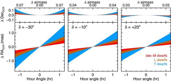
Figure 1. Astrometric offsets in J band due to the differential chromatic refraction (DCR) between our targets and background stars computed for Mauna Kea. These offsets result from our targets' J-band spectra being dissimilar from those of background stars, and thus the offsets increase at later spectral types because the differences are more pronounced. Each colored swath shows the range of offsets predicted for the variety of subtypes within each spectral classification (e.g., T0–T8 for the T dwarfs). The offsets increase with airmass, so our observations were constrained to be as close to transit as possible, and the effects are expected to be worse for targets farther from zenith (δ = 19 8 at Mauna Kea). By always obtaining data within 1 hr of transit (and typically within 30 minutes), we have ensured that the effects of DCR on our astrometry are negligible (≲ 1 mas).
Download figure:
Standard image High-resolution imageThe other major advantage afforded by queue service mode is the ability to obtain excellent parallax phase coverage for targets widely distributed on the sky with minimal impact from poor weather or seeing. Note, however, that WIRCam is bolted onto the telescope when in use and must be removed to use other instruments, so there are discrete WIRCam runs of ≈1–2 weeks each undertaken ≈4–5 times per semester. These runs could be at irregular intervals, depending on the queue pressure each semester. This, combined with the fact that a string of very poor weather could cripple a given run, means that targets at some right ascensions received much better phase coverage in our program than others, with targets at 12h–01h generally getting the most coverage and targets at 04h–10h getting somewhat less.
2.1. Creating an Astrometric Catalog at Each Epoch
2.1.1. Position Measurements
At each epoch we obtained ≈20–30 individual dithered frames of our target fields. We obtained positional measurements for all of the sources in each field from SExtractor (Bertin & Arnouts 1996) using the "windowed" parameters (e.g., XWIN_IMAGE) rather than the classic isophotal parameters (e.g., X_IMAGE). Windowed parameters have the advantage of being less noisy, because they are computed with a Gaussian weight function that decreases the impact of pixels far from the point-spread function (PSF) core on the measured positions. We used flag maps within SExtractor to track sources that were either saturated or located near bad pixels, as identified by the CFHT data processing pipeline. These flagged sources were excluded from subsequent analysis. We also used the signal-to-noise (S/N) estimates from SExtractor6 to exclude sources with S/N < 10. We did not attempt to exclude galaxies based on SExtractor shape parameters at this stage, but in a later step (Section 2.2) nonstellar sources typically ended up being excised because of their large positional rms.
2.1.2. Cross-identifying Detections
The first step in creating an astrometric catalog was to associate all of the detections across multiple frames as belonging to a common set of objects. We found that the most robust method for cross-identifying stars was to first match detections in a given frame to an astrometric reference catalog, either the Sloan Digital Sky Survey Data Release 7 (SDSS-DR7; Abazajian et al. 2009), the Two Micron All Sky Survey Point Source Catalog (2MASS-PSC; Skrutskie et al. 2006), or the USNO-B1.0 Catalog (Monet et al. 2003). We used the information in the CFHT FITS headers to obtain an initial guess for the image coordinates, and we refined this initial guess by using the catalog matching software SCAMP (Bertin 2006). We thereby determined approximate source positions in celestial coordinates, adequate for cross-identifying detections that have corresponding entries in the reference catalog; we used whichever catalog gave the most matches for a target field. We then determined a more precise astrometric solution for the given frame that included second-order terms (i.e., x2, y2, xy) since these distortion terms are significant at the ≈1'' level. This fit was performed using the MPFIT implementation of the Levenberg–Marquardt least-squares minimization routine in IDL (Markwardt 2009). This temporary best-fit astrometric solution was then applied to all the detections in the frame so that we could crossmatch them between frames.
We constructed our catalog of associated detections by starting with the list of detections in the first image and then adding detections from the next image by either finding a match in the existing catalog or creating a new entry if no match was found. After adding a new image, the catalog position of each object was recomputed as the median of currently associated measurements. This procedure was repeated for each image until all positional measurements from that epoch were included in the catalog. We then discarded objects from the catalog that were detected fewer than 10 times in order to focus on stars that will have the most robust astrometry. This cut excludes stars on the periphery of the field that were only captured in a subset of dithers as well as bright sources near the saturation limit and image artifacts (e.g., cosmic rays, persistence spots, and array defects). Note that because we created a separate catalog for each epoch, sources with large proper motion would not be discarded at this step.
2.1.3. Registering Dithers
We next optimally registered the positions of stars cross-associated in individual images at a given epoch. The only information we used from the initial pass of reference catalog matching were the coordinates of the tangent point and linear terms for the first frame, and these were only a temporary guess because later in our analysis we solve for all of these parameters directly. Our optimization operates in spherical rather than (x, y) coordinates in order to properly account for the fact that our measurements are actually tangent projections of celestial positions. For example, our largest dithers of 1' can cause the relative positions of stars at the edges of our 10' field to appear to move by ∼10 mas due to tangent projection effects. The best-fit registration solution was found using MPFIT to jointly minimize unweighted residuals in right ascension, (α − mean(α))cos δ, and declination, δ − mean(δ). The only parameters allowed to vary between frames in this fit were the (α, δ) coordinates of the tangent point (i.e., only a shift). After performing the fit the first time, we clipped any positional measurements that were more than 3.5σ discrepant with the median catalog position to eliminate corrupted measurements (e.g., affected by a cosmic ray hit) or image artifacts that were erroneously associated with real sources. This cut was chosen because it would eliminate ≲ 1 true measurement even in our richest data sets of a few × 103 detections, and typically ≲ 10 detections were actually clipped. After clipping, the fit was then repeated a second and final time.
2.1.4. Accounting for Distortion and Linear Terms
In optimizing the registration of dithers, we allowed for optical distortion as a third-order polynomial function in x and y, which was applied before the tangent projection. These distortion terms were derived from several data sets of the densest target field that lies within the Sloan footprint (2MASS 0850+1057) by fitting our measured (x, y) positions to SDSS-DR7 reference catalog coordinates. SDSS provides the best combination of source density on the sky and positional accuracy (≈40 mas as judged from the rms of our fits) among astrometric reference catalogs currently available. The residuals of our fits using first-, second-, and third-order terms are shown in Figure 2. There was no discernable improvement by including fourth-order terms, so we adopted the best-fit terms up to third order for our distortion solution, shown in Figure 3 with coefficients given in Table 2. We note that we also tried fitting for the distortion from our data alone, since dithered images can in principle constrain any nonlinear terms (e.g., Anderson & King 2003). However, the largest observed offset of any given star between two of our 1' dithers is only ≈2–3 pixels, even though the largest absolute offsets due to distortion are ≈10–20 pixels. Thus, we found that we have more leverage for determining the distortion by using a comparison to an absolute reference catalog. The scatter in the best-fit distortion terms determined from different data sets of 2MASS 0850+1057 reflects this fact as it is much lower for the catalog-matching approach compared with using the internal position residuals alone. We also tested the stability of the distortion pattern by both fixing and fitting for it in dense fields observed throughout our program. The astrometric residuals of star positions did not change significantly, validating our approach of using a single distortion solution for all images.
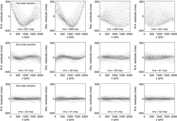
Figure 2. Residuals in the fit of measured WIRCam star positions to the SDSS-DR7 catalog, using linear and higher order distortion terms, as a function of the x and y position. The data set shown here is for ≈200 stars in the 2MASS J0850+1057 field observed over 21 dithers with offsets of 1'. Both second- and third-order terms are needed in the distortion solution, and the resulting residual rms is ≈40 mas, dominated by SDSS positional errors. There is no obvious remaining structure in the residuals, indicating that a third-order solution is sufficient for WIRCam.
Download figure:
Standard image High-resolution image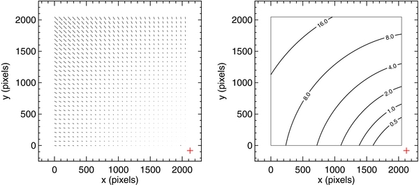
Figure 3. Left: map of the optical distortion present in the northeast array of the WIRCam mosaic (the only array we use). Positional offsets due to distortion are multiplied by 3 to make them more easily visible. The largest distortion offset has an amplitude of 27 pixels (i.e., from corner to corner), but the actual shifts induced in our dithered data sets are at most 1–2 pixels because our largest dithers are ≈200 pixels. Right: contour plot showing how the distortion amplitude increases radially from the optical axis (red cross), which is roughly the midpoint of the four-array WIRCam mosaic. Contours are labeled with the amplitude of the offset in pixels.
Download figure:
Standard image High-resolution imageTable 2. Distortion Coefficients for WIRCam Northeast Array
| Term | aij | bij |
|---|---|---|
| x2 |  |
−6.409 × 10⁻⁷ |
| xy | −1.303 × 10⁻⁶ |  |
| y2 |  |
−1.191 × 10⁻⁶ |
| x3 | −5.287 × 10⁻¹⁰ | −1.466 × 10⁻¹⁰ |
| x2y | −4.130 × 10⁻¹⁰ | −4.589 × 10⁻¹⁰ |
| xy2 | −5.338 × 10⁻¹⁰ | −3.884 × 10⁻¹⁰ |
| y3 | −1.353 × 10⁻¹⁰ | −5.872 × 10⁻¹⁰ |
Notes. To apply this distortion correction, the origin must first be redefined as the optical axis: where x and y are the pixel positions measured by SExtractor. Distortion-free positions may then be computed:
 This distortion correction only applies for the northeast array in the WIRCam mosaic.
Download table as: ASCIITypeset image
We also accounted for differential aberration and refraction offsets in the process of registering dithered images. Both effects are essentially a linear transformation of star positions, since stars on one side of our 10' field experience slightly different positional offsets due to annual stellar aberration and atmospheric refraction than the opposite side of the field. Differential refraction can cause up to a few × 10−4 expansion of the scale along the elevation axis, and differential aberration can cause up to a ±2 × 10⁻⁴ seasonal change in the scale. Thus, it is important to account for these effects in order to monitor the stability of WIRCam's linear terms over time and between targets. We computed the appropriate offsets from equations in Kovalevsky & Seidelmann (2004, pp. 121–141) and applied the differential values (i.e., with the median offset subtracted) to the celestial coordinates in our minimization routine.
2.1.5. Resulting Positional Errors
The end product of combining measurements from each dithered data set was a catalog of median positions in celestial coordinates7 and the rms for each source as determined from ⩾10 dithered measurements. These rms values correspond to the often quoted astrometric quality metric of the "mean error for a single observation of unit weight" (m.e.1). Monet et al. (1992) quote m.e.1 values of 3–5 mas for the highest S/N stars in the USNO CCD program, Vrba et al. (2004) quote 8–10 mas for the brightest reference stars in the USNO infrared astrometry program, and Tinney et al. (2003) report a median rms of 12 mas for the NTT infrared astrometry program. The ultimate astrometric precision at each epoch may be expected to scale as  , and the USNO CCD, USNO IR, and NTT programs obtained 1–2, 3, and 8 frames per epoch, respectively. Therefore, their precisions per epoch are 2–4 mas, 5–6 mas, and 4 mas, respectively. For our program, the rms of the position measurements for our targets were typically 6–18 mas (13 mas median; Figure 4). Because we obtained 20–30 frames for each data set, our astrometric precision per epoch is 1.5–3.0 mas (2.8 mas median). Thus, the quality of our astrometry is comparable to or better than previous ground-based parallax programs targeting ultracool dwarfs in the optical or infrared.

Figure 4. Left: distribution of the FWHM of our observations. The median FWHM for our target within each dithered data set at each epoch is plotted, so the total number of frames we obtained is actually 20–30 times the number of measurements shown here. Middle: distribution of the rms of measured positions among each dithered data set. Right: distribution of the standard error (i.e., rms/ ) of our position measurements at each observation epoch.
Download figure:
Standard image High-resolution image2.2. Registering Astrometry between Epochs
In order to obtain multi-epoch astrometry for all objects in each of our target fields, we next associated the sources measured in different dithered data sets. We excluded the noisiest measurements from this analysis, typically applying an rms threshold of 30–60 mas (0.1–0.2 pixels). The positional shifts between epochs were estimated using a two-dimensional histogram approach as follows: all n1 objects from the first image were each paired with all n2 objects from a second image; the α and δ offsets between all n1 × n2 possible pairings were computed and binned in a two-dimensional histogram; the peak bin in (Δα, Δδ) space, which contains the min(n1, n2) true pairings, was found; the shift was computed by taking the median of the offsets contained in the peak bin. The bin size used was initially set to be arbitrarily large and then iteratively decreased until the number of pairs in the peak bin was <2 times the expected number (i.e., until true pairs dominated the peak bin). The crossmatching of positions was then performed in a similar fashion as for the individual dithered images: a match radius of 20 was employed to associate objects detected at different epochs. Such a large match radius is needed if the proper motion is large (≳ 1'' yr−1), as is the case for some targets. We excluded sources from the multi-epoch astrometry catalog if they were detected at fewer than half of the epochs. This excludes faint sources that were only well detected in the best conditions, bright sources that were only below the saturation limit in poor conditions, and any other transient sources or long-lived artifacts that may be in the data set.
Because the initial association of object positions was based only on rough estimates of the position offsets between epochs, we optimized this registration by fitting for the offsets as well as allowing for relative changes in linear terms across different data sets. Thus, we replaced the initial guesses of the linear terms generated by the reference catalog matching (except for the first epoch, which we solve for later). We parameterized the linear terms as a rotation, x-axis pixel scale, ratio of y/x-axis pixel scales, and a shear term (Δy∝x). We used MPFIT to perform an unweighted least-squares minimization in a similar fashion as described for the dither matching in the previous section. After the first optimization, we fit every object in the field for proper motion and parallax and temporarily excluded objects that displayed significant parallax (>3σ) or proper motion (>30 mas yr−1). This automated procedure typically excluded no more than 5% of the reference stars, and it always excluded the science target. We then determined the optimal registration solution a second and final time after excluding these objects.
2.3. Absolute Astrometric Calibration
We have performed as much of our analysis as possible using relative astrometry in order to preserve the fidelity of our position measurements. However, we must ultimately tie our astrometry to an absolute reference frame in order to determine, e.g., the actual pixel scale and orientation of our images. The most suitable catalogs for this purpose are 2MASS, which provides positions for infrared sources over the entire sky, and SDSS, which has a higher sky density of sources and higher astrometric precision but more limited sky coverage. In our shallowest images taken with the KH2-band filter, we found that shallower reference catalogs were usually more appropriate (USNO-B1, Monet et al. 2003; and UCAC-3, Zacharias et al. 2010). For each field, we constructed a reference frame from the catalog that had the most sources in common with our images. We required reference catalog sources to have absolute position errors ⩽150 mas (e.g., for 2MASS: ERRMAJ < 015). We found the rough offset between our own astrometric catalog and the reference sources by using our aforementioned two-dimensional histogram approach. We then matched reference sources to our own using a match radius of 20. We excluded from this analysis any sources in our astrometric catalog that displayed significant proper motion (>30 mas yr−1), as these would have introduced substantial scatter (≳03) to our comparison with reference catalog position measurements from typically ≈5–10 years ago.
Using the sources in common between our science images and the reference catalog (typically ≳ 30 stars; see Table 1), we determined the absolute astrometric frame for our CFHT images. We registered our positions to the reference catalog, allowing for an offset (i.e., to determine the absolute coordinates of our astrometry) and the linear terms. This solution allows us to compute the pixel scale and orientation in an absolute sense, completely replacing the temporary guess from the initial catalog crossmatching. In the final best-fit registration, the rms of all stars about their catalog positions was typically 60–80 mas for 2MASS and 30–50 mas for SDSS. This scatter is dominated by the reference catalog positional errors. (Thus, the actual relative astrometric uncertainties of 2MASS positions over our 10' field are a factor of ∼2 smaller than the nominal catalog errors of 100–150 mas.) After this final absolute calibration we found that our input guess for the absolute coordinates from image headers was accurate to within ≲ 1''.
2.3.1. Astrometric Stability of WIRCam
The best-fit parameters from the registration of multi-epoch data sets to an astrometric reference catalog enable us to assess the long-term astrometric stability of WIRCam. The level of precision with which we are able to monitor the changes in linear terms such as scale and rotation is fundamentally limited in two ways: (1) positional errors both in our data and reference catalogs introduce random and systematic errors in the derived terms and (2) the uncertainty in the higher order distortion terms is a source of systematic error in the derived linear terms. We have assessed the level of uncertainty in the scale introduced by both of these effects through Monte Carlo simulations. To test the contribution of random errors alone (i.e., case 1), we simulated many star fields with random positions distributed uniformly over a 10' × 10' field and found the best-fit scale to match them to a reference catalog that had normally distributed noise added to it. For a reference catalog accurate to 80 mas (i.e., akin to 2MASS), ≈30 reference stars were needed to achieve a fractional precision in the scale of 1 × 10⁻⁴ (Figure 5). This situation is typical of about half of our targets. For a higher fidelity reference catalog accurate to 40 mas (e.g., like SDSS), 30 reference stars give a much better scale precision of 5 × 10⁻⁵, and the very best case among our targets of 190 SDSS reference stars would give a precision of 2 × 10⁻⁵.
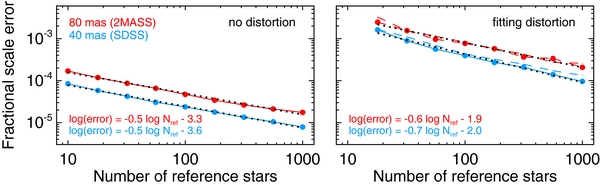
Figure 5. Left: error in the derived pixel scale of WIRCam due only to random errors in the catalog positions as determined from our Monte Carlo simulations. If the distortion of WIRCam were known perfectly, this would set the limit on how well the pixel scale is known, i.e., a fractional uncertainty of 2 × 10⁻⁵ for our calibration field containing ≈200 SDSS stars. (Dashed lines show first-order polynomial fits to the simulation results.) Right: same as the left except that the third-order distortion terms have been treated as free parameters. Because of the strong degeneracy between linear and higher order terms in the fit, the precision in the pixel scale is more than an order of magnitude worse than in the case of no (or known) distortion. This fundamentally limits our absolute calibration of WIRCam to a precision of 3 × 10⁻⁴.
Download figure:
Standard image High-resolution imageThe second source of error present in our determinations of linear terms is the uncertainty in the distortion solution. This is because the linear and higher order terms are partially degenerate when fitting polynomials for the distortion. In the reduction procedure described above, we used data sets containing ≈200 SDSS reference stars to determine the WIRCam distortion, and the catalog errors were estimated to be 40 mas from the rms of the fit residuals. Thus, we simulated many random star fields each containing 200 stars with normally distributed noise of 40 mas and found that fitting freely for both linear and distortion terms resulted in a scale uncertainty of 3 × 10⁻⁴ (Figure 5). This result is effectively independent of the assumed centroiding error in the star positions even up to our worst errors of 0.1 pixel because the reference catalog scatter dominates. This source of error is a few times larger than the uncertainty due simply to random errors in the reference catalog, and thus it is the limiting factor in our ability to measure the scale of WIRCam. From these simulations, the limiting systematic uncertainties in shear and rotation are 3 × 10⁻⁴ and 002 (i.e., 3 × 10⁻⁴ radians), respectively.
With these results in mind, we can now assess the stability of WIRCam from our astrometric monitoring data (Figure 6). (1) We are most sensitive to changes in the orientation of WIRCam and found a highly significant scatter of ±014 among data sets taken over our program. This scatter is clearly not Gaussian but rather is highly correlated with the observation date; the orientation of data sets taken on the same WIRCam observing run was nearly identical. This is consistent with the fact that the instrument is taken off of the telescope between observing runs. (2) We found the x pixel scale to be 030614 ± 000008 pixel−1 (i.e., a fractional error of 3 × 10⁻⁴). Given the errors estimated above, this scatter is consistent with the pixel scale being constant over the duration of our program. This stability is impressive given that WIRCam is taken on and off the telescope for ∼8 observing runs per year. (3) We found the ratio between y and x pixel scales to be consistent with unity (0.9997 ± 0.0003), and the scatter in this value is consistent with the uncertainty given by our Monte Carlo simulations. (4) Finally, we found a significant shear term (which we have defined as Δy∝x) of −0.0013 ± 0.0004. If the angle between WIRCam's x and y axes were different from the 90° angle between north and east only by a rotation, this term would be zero. Instead, this shear term implies that the angle between WIRCam's x and y axes is actually 8993 ± 002 when projected onto the sky.
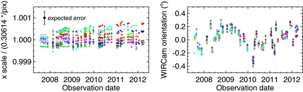
Figure 6. Top: relative pixel scale of the x-axis of WIRCam over the duration of our observing program, with diamonds of different colors indicating different targets (not uniquely since there are 49 targets and only 11 colors). The scatter is consistent with the expected error in linear terms due to the uncertainty in the distortion solution (3 × 10⁻⁴, illustrated by black diamond and error bar). Bottom: orientation of WIRCam over the course of our observing program (0° corresponds to the y axis aligned with north). Changes in the orientation are clearly evident and are correlated with the observing run. (Runs can be seen as groupings of points very close together in time.) This is expected as WIRCam is taken off the telescope between runs.
Download figure:
Standard image High-resolution image2.4. Parallax and Proper Motion Determination
Using our final astrometric catalog of WIRCam position measurements calibrated against an absolute reference frame, we fit for the proper motion and parallax of all sources in each target field. For each source, we used MPFIT to perform a least-squares minimization weighted by the standard errors of the position measurements. We fitted three parameters to the combined (α, δ) data: proper motion in right ascension (μα), proper motion in declination (μδ), and parallax (π). This is notably different from one standard approach taken in the literature of fitting two separate values of the parallax in α and δ. The parallax offsets were computed as follows:


where X, Y, and Z are the coordinates of the Earth relative to the barycenter of the solar system as given by the JPL ephemeris DE405. MPFIT minimized the residuals in (α, δ) after subtracting the relative parallax and proper motion offsets (three parameters) and the mean (α, δ) position (effectively removing 2 additional degrees of freedom). Thus, each fit to 2 × Nepoch measurements had 2 × Nepoch − 5 degrees of freedom (dof).
For each target, we then performed a Markov Chain Monte Carlo (MCMC) analysis on the astrometry in order to accurately determine the posterior distributions of all parameters. We adopted the formalism described by Ford (2005), which uses a Metropolis–Hastings jump acceptance criterion with Gibbs sampling that chooses only one parameter (at random) to be altered at each step in the chain. Before running our science chains, we first ran a test chain to determine the optimal step size (β) for each of our parameters in order to ensure efficient convergence. This initial chain was run according to the procedure outlined by Ford (2006) in which each value of β is periodically adjusted until the acceptance rate for that parameter comes within some tolerance (we chose 5%) of the target rate (we chose 0.25). We then ran 30 chains of 104 steps, each one starting at different points in parameter space drawn at random by adding Gaussian noise, with σ equal to the step size, to the best-fit parameters from the MPFIT results. We computed the Gelman–Rubin statistic for our set of 30 chains, which Ford (2005) suggests should be <1.2 to ensure that the results are converged and well mixed. The Gelman–Rubin statistic was always <1.03 for all parameters, and typically <1.01. Finally, we discarded the first 10% of each chain as the "burn in" portion, using only the latter 90% for deriving the probability distributions of parameters.
At this stage we investigated the impact of DCR on our resulting parallaxes for targets observed in the J band. We assumed an effective wavelength of 1.2462 μm for the background star reference frame, based on the typical values for GKM stars as discussed earlier, and computed individual DCR offsets for the measured positions at each epoch using the method described in the introduction to this section (also see Figure 1). We added these offsets to the measured astrometry and performed our MCMC analysis a second time. We found that the change in the resulting parallax was almost always ⩽0.15σ. As a source of systematic error this is completely negligible as it would boost the final error by ⩽1% when added in quadrature. In a few special cases that are most sensitive to DCR shifts (i.e., three T7–T8 dwarfs with fewer than 10 epochs) the change in parallax was as large as 0.2σ–0.4σ. This would give a slightly larger boost of 2%–7% to their errors, but this is still negligible. In examining the ensemble of the 33 J-band targets for which we computed DCR parallax offsets, we found a mean±rms offset of −0.10 ± 0.19 mas (−0.06 ± 0.10 mas when excluding objects with parallax errors >2 mas), indicating that there is also no systematic offset in our parallaxes due to DCR.
We also performed tests on our data to determine when to consider a parallax measurement "done." Even though our MCMC analysis fully captures any uncertainty due to the degeneracy between proper motion and parallax over data sets spanning modest time baselines (≲ 2 years), we wanted to confirm that the parallaxes we present here will not change substantially with the addition of future data. To check this, for each object we determined the best-fit parallax using subsets of the data starting with the first three epochs (the minimum needed to constrain the five-parameter fit) and then adding one data point at a time for each successive epoch. As expected, the most important criterion for reaching a stable parallax solution was the time baseline. For all of our targets we found that a time baseline of ≈1.2 years was sufficient to reach a best-fit parallax value that remained stable with the addition of new data up to the last observation epoch (our longest time baseline to date is 4.3 years). Therefore, all of the parallaxes presented here are expected to have reached a stable, final value (median baseline of 2.4 years, minimum 1.8 years). We note that this minimum needed time baseline of 1.2 years will necessarily be longer for cases where the astrometric errors are significantly larger than ours or when the target parallax is smaller.
The results from our MCMC analysis are given in Table 3, and the astrometric data are shown in Figures 7–8. The minimum χ2 value for each chain is commensurate with the degrees of freedom, which verifies that our adopted positional errors are accurate. There are three exceptions, the known binaries 2MASS J0518−2828AB (Burgasser et al. 2006c) and 2MASS J1404−3159AB (Looper et al. 2008) and the candidate unresolved binary SDSS J0805+4812 (Burgasser 2007b). Their large χ2/dof values can be attributed to the large perturbations present in the residuals after fitting for parallax and proper motion due to orbital motion.
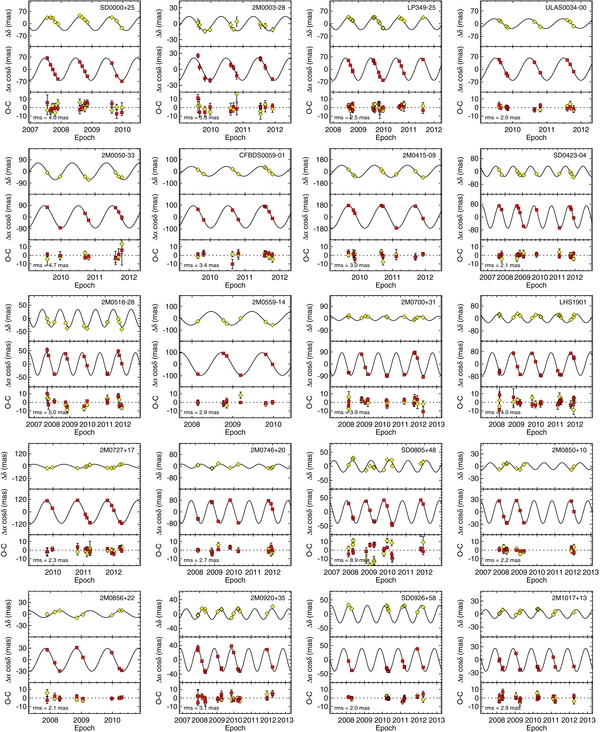
Figure 7. For each object, the top and middle panels show relative astrometry in δ and α, respectively, as a function of Julian year after subtracting the best-fit proper motion. (This is for display purposes only; in our analysis we fit for both the proper motion and parallax simultaneously.) The bottom panels show the residuals after subtracting both the parallax and proper motion.
Download figure:
Standard image High-resolution image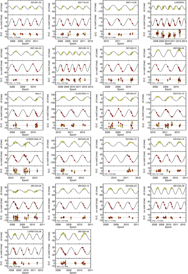
Download figure:
Standard image High-resolution image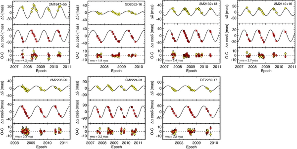
Figure 8. Same as Figure 7.
Download figure:
Standard image High-resolution imageTable 3. Parallax and Proper Motion MCMC Results
| Target | αJ2000 | δJ2000 | Epoch | μαcos δ | μδ | μ | P.A. | πabs | χ2/dof |
|---|---|---|---|---|---|---|---|---|---|
| (deg) | (deg) | (MJD) | ('' yr−1) | ('' yr−1) | ('' yr−1) | (deg) | ('') | ||
| SDSS J000013.54+255418.6 | 000.0563857 | +25.9054561 | 54301.63 | −0.0191(15) | 0.1267(13) | 0.1281(13) | 351.4 ± 0.7 | 0.0708(19) | 22.5/19 |
| 2MASSI J0003422−282241 | 000.9277249 | −28.3782531 | 55050.53 | 0.2803(15) | −0.1233(17) | 0.3062(15) | 113.7 ± 0.3 | 0.0250(19) | 21.4/17 |
| LP 349-25AB | 006.9841925 | +22.3255463 | 54687.57 | 0.4040(10) | −0.1654(15) | 0.4365(9) | 112.27 ± 0.21 | 0.0696(9) | 23.2/25 |
| ULAS J003402.77−005206.7 | 008.5116117 | −00.8687246 | 55051.60 | −0.0167(10) | −0.3588(8) | 0.3592(8) | 182.66 ± 0.16 | 0.0687(14) | 13.3/13 |
| 2MASS J00501994−3322402 | 012.5872589 | −33.3749337 | 55050.57 | 1.1505(22) | 0.9391(21) | 1.4851(21) | 50.78 ± 0.08 | 0.0946(24) | 10.2/9 |
| CFBDS J005910.90−011401.3 | 014.7960832 | −01.2335758 | 55068.57 | 0.8847(11) | 0.0440(13) | 0.8858(11) | 87.15 ± 0.08 | 0.1032(21) | 11.7/11 |
| 2MASSI J0415195−093506 | 063.8381022 | −09.5835266 | 55070.64 | 2.2143(12) | 0.5359(12) | 2.2782(12) | 76.39 ± 0.03 | 0.1752(17) | 13.6/11 |
| SDSSp J042348.57−041403.5AB | 065.9516865 | −04.2338814 | 54341.64 | −0.3276(5) | 0.0912(5) | 0.3401(5) | 285.56 ± 0.09 | 0.0721(11) | 12.5/17 |
| 2MASS J05185995−2828372AB | 079.7498449 | −28.4773438 | 54366.66 | −0.0700(5) | −0.2757(5) | 0.2844(5) | 194.25 ± 0.10 | 0.0437(8) | 73.3/19 |
| 2MASSI J0559191−140448 | 089.8314377 | −14.0809294 | 54519.25 | 0.5718(15) | −0.3330(17) | 0.6617(16) | 120.21 ± 0.14 | 0.0966(10) | 8.2/7 |
| 2MASS J07003664+3157266AB | 105.1532663 | +31.9561584 | 54513.30 | 0.1424(7) | −0.5546(7) | 0.5726(7) | 165.60 ± 0.07 | 0.0867(12) | 20.4/19 |
| LHS 1901AB | 107.7986681 | +43.4984000 | 54513.31 | 0.3544(8) | −0.5662(9) | 0.6680(9) | 147.96 ± 0.08 | 0.0742(10) | 29.3/27 |
| 2MASSI J0727182+171001 | 111.8296673 | +17.1646091 | 55125.63 | 1.0470(9) | −0.7642(10) | 1.2962(9) | 126.12 ± 0.04 | 0.1125(9) | 18.4/19 |
| 2MASSI J0746425+200032AB | 116.6763725 | +20.0089457 | 54517.34 | −0.3659(7) | −0.0527(5) | 0.3697(7) | 261.81 ± 0.08 | 0.0811(9) | 18.4/15 |
| SDSS J080531.84+481233.0 | 121.3813807 | +48.2094111 | 54428.60 | −0.4583(7) | 0.0498(8) | 0.4610(7) | 276.20 ± 0.09 | 0.0431(10) | 229.1/21 |
| 2MASSs J0850359+105716AB | 132.6494655 | +10.9544494 | 54428.61 | −0.1442(6) | −0.0126(6) | 0.1447(6) | 265.01 ± 0.24 | 0.0301(8) | 18.6/13 |
| 2MASSI J0856479+223518AB | 134.1992240 | +22.5884467 | 54428.62 | −0.1869(10) | −0.0133(8) | 0.1874(10) | 265.95 ± 0.24 | 0.0324(10) | 8.6/11 |
| 2MASSW J0920122+351742AB | 140.0506337 | +35.2949198 | 54427.66 | −0.1889(8) | −0.1984(6) | 0.2740(8) | 223.59 ± 0.13 | 0.0344(8) | 24.2/25 |
| SDSS J092615.38+584720.9AB | 141.5641928 | +58.7888671 | 54513.41 | 0.0102(5) | −0.2162(5) | 0.2165(5) | 177.30 ± 0.12 | 0.0437(11) | 21.0/17 |
| 2MASSI J1017075+130839AB | 154.2817771 | +13.1442355 | 54514.44 | 0.0479(5) | −0.1178(5) | 0.1272(5) | 157.86 ± 0.24 | 0.0302(14) | 29.7/21 |
| SDSS J102109.69−030420.1AB | 155.2902375 | −03.0722820 | 54514.45 | −0.1626(6) | −0.0745(7) | 0.1789(6) | 245.38 ± 0.21 | 0.0299(13) | 13.7/13 |
| SDSS J111010.01+011613.1 | 167.5412045 | +01.2699602 | 54514.50 | −0.2171(7) | −0.2809(6) | 0.3550(7) | 217.71 ± 0.11 | 0.0521(12) | 18.6/15 |
| 2MASS J11145133−2618235 | 168.7032979 | −26.3074976 | 55280.39 | −3.0188(11) | −0.3841(14) | 3.0432(11) | 262.75 ± 0.03 | 0.1792(14) | 12.8/9 |
| LHS 2397aAB | 170.4539114 | −13.2189698 | 54520.49 | −0.4869(25) | −0.0614(16) | 0.4908(23) | 262.81 ± 0.21 | 0.0730(21) | 28.3/21 |
| 2MASSW J1146345+223053AB | 176.6440817 | +22.5151927 | 54514.51 | 0.0256(7) | 0.0894(8) | 0.0930(8) | 16.0 ± 0.4 | 0.0349(10) | 9.4/9 |
| 2MASS J12095613−1004008AB | 182.4851412 | −10.0678779 | 54513.52 | 0.2661(5) | −0.3554(6) | 0.4440(6) | 143.18 ± 0.06 | 0.0458(10) | 24.8/19 |
| DENIS-P J1228.2−1547AB | 187.0639038 | −15.7935333 | 54514.54 | 0.1344(8) | −0.1853(10) | 0.2289(9) | 144.04 ± 0.22 | 0.0448(18) | 15.1/17 |
| 2MASSW J1239272+551537AB | 189.8644820 | +55.2605441 | 54513.53 | 0.1252(11) | −0.0004(11) | 0.1252(11) | 90.2 ± 0.5 | 0.0424(21) | 18.0/13 |
| Kelu-1AB | 196.4167629 | −25.6847666 | 54514.56 | −0.2992(12) | −0.0041(14) | 0.2992(12) | 269.21 ± 0.28 | 0.0497(24) | 15.9/13 |
| ULAS J133553.45+113005.2 | 203.9727703 | +11.5014079 | 55287.48 | −0.1908(15) | −0.2024(13) | 0.2782(12) | 223.3 ± 0.3 | 0.0999(16) | 14.2/15 |
| 2MASS J14044948−3159330AB | 211.2070713 | −31.9923990 | 54515.60 | 0.3448(10) | −0.0107(14) | 0.3450(10) | 91.79 ± 0.23 | 0.0421(11) | 118.5/17 |
| SDSS J141624.08+134826.7 | 214.1008726 | +13.8080084 | 55307.42 | 0.0952(13) | 0.1329(15) | 0.1635(14) | 35.6 ± 0.5 | 0.1097(13) | 25.4/21 |
| CFBDS J145829+10134AB | 224.6224723 | +10.2283899 | 55283.56 | 0.1740(20) | −0.3818(27) | 0.4196(26) | 155.50 ± 0.28 | 0.0313(25) | 22.4/17 |
| 2MASSW J1503196+252519 | 225.8321432 | +25.4236612 | 54575.47 | 0.0901(16) | 0.5618(16) | 0.5690(16) | 9.11 ± 0.16 | 0.1572(22) | 10.6/9 |
| SDSS J150411.63+102718.3 | 226.0493096 | +10.4545909 | 55050.24 | 0.3736(19) | −0.3692(21) | 0.5253(19) | 134.66 ± 0.22 | 0.0461(15) | 10.6/7 |
| SDSS J153417.05+161546.1AB | 233.5710654 | +16.2629914 | 54515.65 | −0.0799(7) | −0.0362(8) | 0.0877(7) | 245.7 ± 0.5 | 0.0249(11) | 19.6/17 |
| 2MASSI J1534498−295227AB | 233.7082531 | −29.8747002 | 54515.66 | 0.0934(9) | −0.2600(13) | 0.2763(13) | 160.24 ± 0.20 | 0.0624(13) | 28.5/27 |
| 2MASSW J1553022+153236AB | 238.2584798 | +15.5441600 | 54576.51 | −0.3859(7) | 0.1662(9) | 0.4201(7) | 293.30 ± 0.12 | 0.0751(9) | 14.0/11 |
| SDSS J162838.77+230821.1 | 247.1623605 | +23.1387790 | 54576.52 | 0.4123(8) | −0.4430(7) | 0.6052(8) | 137.06 ± 0.07 | 0.0751(9) | 13.9/13 |
| 2MASSW J1728114+394859AB | 262.0481027 | +39.8164269 | 54576.59 | 0.0358(5) | −0.0184(6) | 0.0402(5) | 117.2 ± 0.8 | 0.0387(7) | 23.4/17 |
| LSPM J1735+2634AB | 263.8044568 | +26.5792649 | 54576.60 | 0.1496(8) | −0.3191(8) | 0.3525(8) | 154.88 ± 0.12 | 0.0667(14) | 18.3/13 |
| 2MASSW J1750129+442404AB | 267.5533210 | +44.4019032 | 54576.60 | −0.0152(8) | 0.1433(9) | 0.1441(9) | 354.0 ± 0.3 | 0.0303(10) | 21.8/21 |
| 2MASSI J1847034+552243AB | 281.7647659 | +55.3788062 | 54314.36 | 0.1244(9) | −0.0621(12) | 0.1391(10) | 116.5 ± 0.5 | 0.0298(11) | 26.0/21 |
| SDSS J205235.31−160929.8AB | 313.1476698 | −16.1580321 | 54314.45 | 0.3997(6) | 0.1527(7) | 0.4279(6) | 69.09 ± 0.09 | 0.0339(8) | 24.8/29 |
| 2MASSI J2132114+134158AB | 323.0479693 | +13.6995052 | 54314.50 | 0.0195(13) | −0.1225(8) | 0.1240(7) | 171.0 ± 0.6 | 0.0360(7) | 40.5/43 |
| 2MASSW J2140293+162518AB | 325.1219856 | +16.4217247 | 54314.49 | −0.0686(8) | −0.0827(8) | 0.1075(8) | 219.7 ± 0.4 | 0.0325(11) | 20.6/23 |
| 2MASSW J2206228−204705AB | 331.5952108 | −20.7847199 | 54635.61 | 0.0130(9) | −0.0318(11) | 0.0344(11) | 157.8 ± 1.5 | 0.0357(12) | 31.2/31 |
| 2MASSW J2224438−015852 | 336.1838686 | −01.9830172 | 54316.47 | 0.4685(5) | −0.8648(6) | 0.9836(6) | 151.55 ± 0.03 | 0.0862(11) | 35.4/33 |
| DENIS-P J225210.73−173013.4AB | 343.0457856 | −17.5031008 | 54318.51 | 0.3973(15) | 0.1443(39) | 0.4226(20) | 70.0 ± 0.5 | 0.0632(16) | 24.5/27 |
Notes. This table gives all the astrometric parameters derived from our MCMC analysis for each target. For parameters in units of arcseconds, errors are given in parentheses in units of 10−4 arcsec. (α, δ, MJD): coordinates that correspond to the epoch listed, which is the first epoch of our observations for that target. (μαcos δ, μδ, μ, P.A.): proper motion parameters are listed both as the direct fitting results (i.e., in α and δ) and the computed quantities of total amplitude (μ) and position angle. πabs: the absolute parallax as computed by combining the relative parallax that comes directly from our fits with the relative-to-absolute corrections (see Section 2.4.2). Note that where applicable proper motion and parallax parameters contain orbital motion correction offsets (see Section 2.4.1 and Table 4). χ2/dof: the lowest χ2 in each set of MCMC chains along with the degrees of freedom.
Download table as: ASCIITypeset image
2.4.1. Correction for Orbital Motion
For the binaries in our sample which have orbit determinations, we apply a correction to the best-fit parallax and proper motion parameters to account for photocenter shifts due to orbital motion. All binaries in our sample only have relative astrometric orbit determinations, so the center of mass is not known. Thus, we use the relative orbital offsets and an assumed mass ratio (derived from evolutionary models) to compute the motion of the center of mass. This motion is then modified by a factor that depends on the binary's flux ratio in the bandpass used in our CFHT imaging in order to determine the actual motion of the photocenter. The coefficient by which to multiply the relative orbital motion is thus (ξ − γ), where


l is the flux ratio (≡ f2/f1 = 10−0.4Δm), and q is the mass ratio (≡ M2/M1). The coefficient (ξ − γ) is typically negative because flux is a steeper-than-linear function of mass, and thus the photocenter motion is opposite in sign from that of the orbit of the secondary relative to the primary.
We compute the astrometric offsets in a Monte Carlo fashion, using the Markov chain from the published orbit determination to draw the binary's orbital elements (e.g., see Liu et al. 2008). We also draw random: (1) flux ratios corresponding to the error in the measured J-band resolved photometry of the target binaries (or K-band photometry for targets using the CFHT KH2 filter); and (2) mass ratios from evolutionary models are derived using the method described in Section 5.4 of Dupuy et al. (2009b). Our Monte Carlo approach enables us to appropriately track the correlation between the different parameters (e.g., the derived mass ratio depends on the K-band flux ratio and also the system mass via the orbital elements). For each Monte Carlo trial we subtracted the orbital motion offsets from our CFHT astrometry and recomputed the best-fit parallax and proper motion. This enabled us to derive systematic offsets and corresponding errors due to the uncertainties in the various input parameters.
Our corrections to the parallax and proper motion are given in Table 4 along with the predicted semimajor axis of the photocenter motion for each binary (aphot). We quote aphot as positive for photocenter motion has the same sign as the primary motion. For each target we added the randomly drawn orbital motion offsets to our MCMC chains in a Monte Carlo fashion. We note that the minimum χ2 of the parallax fit either improved or did not change significantly for all binaries. The latter cases correspond to orbital motion that is nearly linear (e.g., for very long period binaries) and thus easily compensated for by a slightly different proper motion than the precorrected fit. The parallax offsets are quite small (always <0.5σπ, median 0.08σπ), which is not surprising since the orbital periods of these binaries are very long (≈10–20 years). The proper motion offsets are much more significant, since the orbital motion over 2–4 years of monitoring can largely be expressed as a linear term. (We note that even though these proper motions are corrected for orbital motion, they are still not "absolute" since the bulk proper motion of the background stars that define the astrometric reference frame is not known.)
Table 4. Orbital Motion Corrections to Parallax and Proper Motion
| Target | aphot | q | Δm | Δμαcos δ | Δμδ | Δμ | ΔP.A. | Δπ | Δχ2 | Orbit |
|---|---|---|---|---|---|---|---|---|---|---|
| (mas) | (M2/M1) | (mag) | ('' yr−1) | ('' yr−1) | ('' yr−1) | (deg) | ('') | Ref. | ||
| LP 349-25AB | 5.0 ± 1.7 | 0.86 ± 0.04 | 0.307 ± 0.008 | 0.0018(6) | 0.0030(10) | 0.0005(2) | −0.46(16) | −0.00040(13) | 0.0 | 3 |
| LP 415-20AB | 10.0 ± 1.1 | 0.80 ± 0.03 | 0.728 ± 0.023 | 0.0026(3) | 0.0000(1) | 0.0025(3) | −0.32(5) | −0.00006(7) | −1.3 | 5 |
| LHS 1901AB | 7.4 ± 1.0 | 1.00 ± 0.00 | 0.113 ± 0.016 | −0.0006(1) | −0.0032(5) | 0.0024(4) | 0.19(3) | 0.00016(5) | 0.0 | 3 |
| 2MASS J0746 + 2000AB | 14.1 ± 1.9 | 0.92 ± 0.02 | 0.356 ± 0.024 | 0.0025(3) | −0.0018(2) | −0.0022(3) | −0.33(4) | −0.00008(2) | 0.0 | 6 |
| 2MASS J0920 + 3517AB | 3.3 ± 1.1 | 0.98 ± 0.02 | 0.25 ± 0.07 | 0.0017(6) | 0.0007(3) | −0.0017(6) | −0.15(5) | −0.00044(18) | −11.8 | 4 |
| LHS 2397aAB | 78 ± 7 | 0.77 ± 0.08 | 2.80 ± 0.03 | 0.0270(24) | −0.0104(12) | −0.0257(22) | −1.51(16) | −0.00081(16) | −19.4 | 2 |
| 2MASS J1534−2952AB | 6.3 ± 2.0 | 0.95 ± 0.03 | 0.162 ± 0.014 | −0.0003(2) | −0.0014(6) | 0.0012(5) | 0.15(7) | −0.00001(3) | −0.2 | 7 |
| 2MASS J2132 + 1341AB | 11.8 ± 2.0 | 0.81 ± 0.07 | 0.85 ± 0.04 | −0.0067(12) | −0.0008(6) | −0.0005(5) | 3.11(57) | 0.00016(9) | −2.2 | 4 |
| 2MASS J2206−2047AB | 2.6 ± 1.6 | 0.99 ± 0.03 | 0.067 ± 0.010 | −0.0004(3) | −0.0000(1) | −0.0001(1) | 0.61(54) | 0.00000(14) | 0.0 | 1 |
| DENIS-P J2252−1730AB | 9 ± 4 | 0.55 ± 0.04 | 0.94 ± 0.07 | 0.0001(8) | 0.0010(37) | 0.0005(16) | −0.10(47) | 0.00001(15) | −4.1 | 4 |
Notes. Offsets to parallax and proper motion parameters due to orbital motion during our astrometric monitoring program. This is computed from the relative orbit parameters (reference given in the last column), our evolutionary model-derived mass ratio estimate (q), and the flux ratio in the observed bandpass (Δm). The semimajor axis of the resulting photocenter motion (aphot) is shown for each binary. The difference in χ2 between the original best-fit astrometric solution and orbit-corrected solution is also given (Δχ2). These offsets and their errors have already been accounted for in values given in Table 3. References. (1) Dupuy et al. 2009a; (2) Dupuy et al. 2009c; (3) Dupuy et al. 2010; (4) Dupuy 2010; (5) Dupuy & Liu 2011; (6) Konopacky et al. 2010; (7) Liu et al. 2008.
Download table as: ASCIITypeset image
The three binaries showing large perturbations due to orbital motion (2MASS J0518−2828AB, SDSS J0805+4812AB, and 2MASS J1404−3159AB) unfortunately do not have orbit determinations, and thus we are unable to correct their astrometry as described in this section. Additional astrometric monitoring is needed before the orbits of these binaries can be determined from CFHT data alone.
2.4.2. Correction from Relative to Absolute Parallax
The final step in determining the parallaxes of our targets is the conversion from relative to absolute parallax. Because our reference objects are almost all stars, not galaxies,8 their finite distances will result in a small parallax motion of the reference frame that erases part of the true parallax motion of our target. This introduces a systematic error in the parallax measurement that varies in amplitude depending on the distance distribution of the reference stars in each target field.
We have computed a correction to account for this effect using the Besançon model of the Galaxy (Robin et al. 2003). Given the celestial coordinates of each field, the Besançon model generates a list of simulated stars with distances, magnitudes, and proper motions. We oversampled the model output for our WIRCam fields by a factor of 40 in order to ensure that our derived corrections are not dominated by small number statistics. For each field, we used the SExtractor photometry to determine the magnitude range of our reference stars, and we used only model stars within this range for our calculations. The distribution of the model star distances for our fields is typically peaked at 0.5–2 kpc, giving corrections of 0.5–2.0 mas (i.e., ≈1–2σπ). We added the model-predicted parallax offsets to the actual reference stars within the analysis pipeline in a Monte Carlo fashion to determine the impact on the final derived target parallax. We found that different approaches such as applying offsets as a function of star brightness, applying offsets randomly, or not applying offsets to a subset of our reference sources (e.g., simulating the fact that some reference sources may be galaxies) all produced essentially the same systematic error in the target parallax. The resulting shift was always very close to the mean of the model-predicted parallax distribution. Thus, we used the mean Besançon parallax for each field as the correction from relative to absolute parallax. We adopted an uncertainty in this correction factor based on sampling variance in a Monte Carlo fashion. For example, if a target field's astrometric catalog contained 100 stars, we drew random subsets of 100 stars from the oversampled Besançon model output and determined the mean Besançon parallax for each trial. The rms of 103 trials was adopted as the error in the absolute parallax correction (median error in the correction was 0.2 mas). In Table 1 we list the values of these corrections derived for our target fields.
3. KECK/NIRC2, HST, AND VLT RESOLVED PHOTOMETRY
We have used the AO system at the Keck II Telescope on Mauna Kea, HI, to resolve 17 binaries in our sample and measure relative photometry. We employed the facility near-infrared camera NIRC2 to obtain images in the standard Mauna Kea Observatories (MKO) photometric system (Simons & Tokunaga 2002; Tokunaga et al. 2002). Depending on the target and observing conditions (see Table 5), we used laser guide star (LGS) AO (Wizinowich et al. 2006; van Dam et al. 2006) or natural guide star (NGS) AO (Wizinowich et al. 2000, 2004). At some epochs we obtained data using the nine-hole non-redundant aperture mask installed in the filter wheel of NIRC2 (Tuthill et al. 2006). Our procedure for obtaining, reducing, and analyzing such imaging and masking data is described in detail in our previous work (e.g., Liu et al. 2006; Dupuy et al. 2009b, 2009c). Table 5 summarizes the Keck observations presented here, and Figures 9–11 show our imaging data.
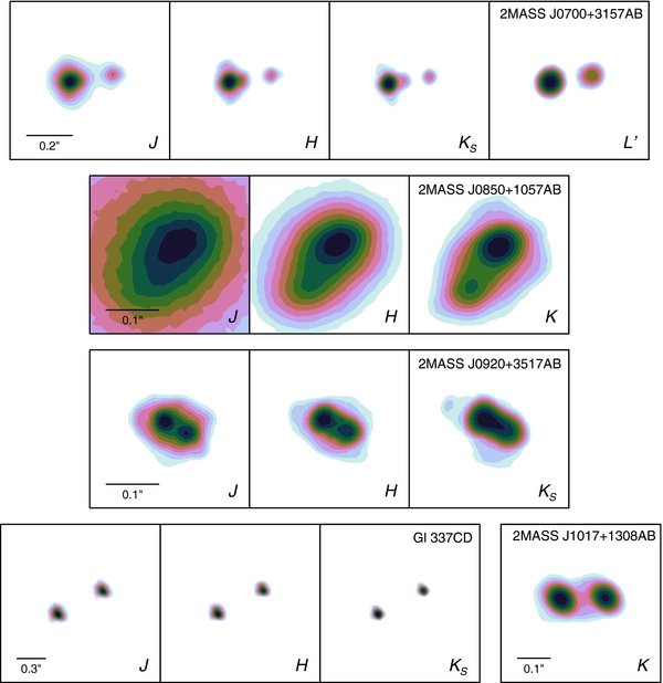
Figure 9. Contour plots of the Keck AO images for which we present resolved photometry in Table 5. Contours are in logarithmic intervals from unity to 10% of the peak flux in each band. North is always up, but the angular scale used for each binary varies, so scale bars are given.
Download figure:
Standard image High-resolution image
Figure 10. Same as Figure 9.
Download figure:
Standard image High-resolution image
Figure 11. Same as Figure 9.
Download figure:
Standard image High-resolution imageTable 5. Keck AO Observations of Sample Binaries
| Target | Epoch | NIRC2 | FWHM | Strehl | Δm |
|---|---|---|---|---|---|
| (UT) | Filter | (mas) | Ratio | (mag) | |
| SDSS J0423−0414AB | 2007 Sep 6 | K | ... | ... | 1.18 ± 0.08 |
| 2MASS J0700 + 3157AB | 2008 Nov 3 | J | 65 ± 5 | 0.026 ± 0.004 | 1.491 ± 0.019 |
| H | 61.0 ± 2.0 | 0.081 ± 0.008 | 1.403 ± 0.017 | ||
| KS | 63.6 ± 1.8 | 0.194 ± 0.021 | 1.390 ± 0.011 | ||
| L' | 86.5 ± 1.4 | 0.61 ± 0.10 | 0.92 ± 0.03 | ||
| 2MASS J0850 + 1057AB | 2006 Dec 19 | J | 58 ± 6 | 0.044 ± 0.004 | 0.82 ± 0.12 |
| H | 58 ± 5 | 0.11 ± 0.02 | 0.80 ± 0.08 | ||
| 2011 Apr 22 | K | ... | ... | 0.91 ± 0.07 | |
| 2MASS J0920 + 3517AB | 2006 May 5 | J | 36.2 ± 1.0 | 0.110 ± 0.011 | 0.25 ± 0.07 |
| H | 39.8 ± 0.5 | 0.23 ± 0.03 | 0.26 ± 0.04 | ||
| KS | 49.0 ± 0.9 | 0.46 ± 0.04 | 0.336 ± 0.023 | ||
| Gl 337CD | 2006 May 4 | J | 89 ± 8 | 0.027 ± 0.008 | 0.18 ± 0.03 |
| H | 94 ± 11 | 0.066 ± 0.016 | 0.20 ± 0.03 | ||
| KS | 87 ± 7 | 0.156 ± 0.019 | 0.27 ± 0.03 | ||
| 2MASS J1017 + 1308AB | 2011 Apr 21 | K | 66 ± 3 | 0.276 ± 0.023 | 0.127 ± 0.010 |
| SDSS J1021−0304AB | 2005 Nov 26 | J | 78 ± 11 | 0.030 ± 0.008 | −0.10 ± 0.03 |
| H | 59 ± 2 | 0.11 ± 0.02 | 0.73 ± 0.03 | ||
| KS | 66 ± 5 | 0.20 ± 0.03 | 1.00 ± 0.03 | ||
| Gl 417BC | 2007 Mar 25 | K | 91 ± 5 | 0.15 ± 0.02 | 0.347 ± 0.025 |
| 2MASS J1225−2739AB | 2010 Jan 10 | J | 90 ± 6 | 0.029 ± 0.002 | 1.317 ± 0.008 |
| H | 100 ± 14 | 0.044 ± 0.013 | 1.490 ± 0.018 | ||
| CH4s | 87 ± 7 | 0.071 ± 0.012 | 1.316 ± 0.011 | ||
| K | 90 ± 7 | 0.15 ± 0.04 | 1.589 ± 0.011 | ||
| DENIS-P J1228−1547AB | 2008 Jun 30 | KS | 108 ± 7 | 0.081 ± 0.010 | 0.137 ± 0.013 |
| 2MASS J1404−3159AB | 2006 Jun 3 | J | 140 ± 30 | 0.012 ± 0.006 | −0.54 ± 0.08 |
| H | 72 ± 5 | 0.091 ± 0.011 | 0.51 ± 0.04 | ||
| KS | 64 ± 3 | 0.296 ± 0.016 | 1.21 ± 0.05 | ||
| 2MASS J1553 + 1532AB | 2010 May 23 | J | 217 ± 11 | 0.010 ± 0.002 | 0.36 ± 0.04 |
| H | 207 ± 14 | 0.014 ± 0.004 | 0.375 ± 0.023 | ||
| CH4s | 218 ± 19 | 0.015 ± 0.003 | 0.32 ± 0.04 | ||
| K | 173 ± 11 | 0.047 ± 0.011 | 0.429 ± 0.025 | ||
| 2MASS J1728 + 3948AB | 2006 Jun 3 | J | 102 ± 14 | 0.020 ± 0.002 | 0.23 ± 0.04 |
| H | 87 ± 7 | 0.057 ± 0.006 | 0.41 ± 0.03 | ||
| KS | 92 ± 7 | 0.11 ± 0.02 | 0.57 ± 0.02 | ||
| LSPM J1735 + 2634AB | 2010 May 23 | J | 88 ± 6 | 0.017 ± 0.007 | 0.57 ± 0.03 |
| H | 80 ± 7 | 0.073 ± 0.019 | 0.557 ± 0.005 | ||
| K | 81 ± 4 | 0.185 ± 0.019 | 0.488 ± 0.011 | ||
| L' | 106 ± 16 | 0.38 ± 0.10 | 0.34 ± 0.03 | ||
| SDSS J2052−1609AB | 2005 Oct 11 | J | 126 ± 39 | 0.029 ± 0.022 | 0.00 ± 0.04 |
| H | 110 ± 16 | 0.062 ± 0.017 | 0.33 ± 0.07 | ||
| K | 88 ± 16 | 0.16 ± 0.06 | 0.85 ± 0.09 | ||
| 2MASS J2132 + 1341AB | 2008 Aug 20 | J | 39.4 ± 1.2 | 0.062 ± 0.016 | 0.85 ± 0.04 |
| H | 44.1 ± 0.8 | 0.157 ± 0.016 | 0.91 ± 0.05 | ||
| 2007 Sep 6 | KS | ... | ... | 0.819 ± 0.023 | |
| 2010 May 10 | K | 52.3 ± 0.9 | 0.43 ± 0.07 | 0.86 ± 0.05 | |
| DENIS-P J2252−1730AB | 2010 Jul 9 | K | ... | ... | 1.72 ± 0.08 |
Notes. Epochs without FWHM or Strehl ratio information correspond to aperture masking observations. The errors on the FWHM and Strehl ratios are the rms scatter among individual dithered images.
Download table as: ASCIITypeset image
We also analyzed HST/NICMOS and VLT/NACO archival images of eight ultracool binaries with parallaxes to supplement our sample of resolved near-IR photometry. Five of these have had their NICMOS data published previously (Golimowski et al. 2004a; Burgasser et al. 2006c, 2011), sometimes without errors given (Reid et al. 2006a). Our re-analysis thus provides a check on the published values and errors. Two of these binaries are among the 17 that we have observed with Keck/NIRC2. Table 6 summarizes the results of our (re)analysis of these archival data.
Table 6. Analysis of Archival Imaging for Sample Binaries
| Target | Epoch | Instrument | Filter | Δm |
|---|---|---|---|---|
| (UT) | (mag) | |||
| GJ 1001BC | 2004 Sep 17 | HST/NICMOS | F110W | 0.10 ± 0.04 |
| F170M | 0.11 ± 0.05 | |||
| 2004 Oct 7 | VLT/NACO | J | 0.10 ± 0.05 | |
| H | 0.15 ± 0.04 | |||
| KS | 0.10 ± 0.05 | |||
| LHS 1070ABa | 2003 Dec 12 | VLT/NACO | J | 0.648 ± 0.036 |
| H | 0.579 ± 0.032 | |||
| KS | 0.453 ± 0.030 | |||
| L' | 0.214 ± 0.025 | |||
| LHS 1070BCa | 2003 Dec 12 | VLT/NACO | J | 0.335 ± 0.009 |
| H | 0.323 ± 0.004 | |||
| KS | 0.321 ± 0.004 | |||
| L' | 0.276 ± 0.029 | |||
| 2MASS J00250365+4759191AB | 2005 May 22 | HST/NICMOS | F110W | 0.187 ± 0.022 |
| F170M | 0.151 ± 0.008 | |||
| DENIS-P J020529.0−115925AB | 2008 Aug 10 | HST/NICMOS | F110W | 0.11 ± 0.18 |
| F170M | 0.098 ± 0.026 | |||
| 2006 Sep 25 | VLT/NACO | KS | 0.110 ± 0.042 | |
| 2MASS J05185995−2828372AB | 2004 Sep 7 | HST/NICMOS | F110W | 0.46 ± 0.25 |
| F170M | 1.09 ± 0.19 | |||
| 2MASSs J0850359+105716AB | 2003 Nov 9 | HST/NICMOS | F110W | 1.15 ± 0.06 |
| F170M | 0.927 ± 0.023 | |||
| SDSS J092615.38+584720.9AB | 2004 Feb 5 | HST/NICMOS | F110W | 0.35 ± 0.07 |
| F170M | 0.66 ± 0.20 | |||
| DENIS-P J225210.73−173013.4AB | 2005 Jun 21 | HST/NICMOS | F110W | 0.98 ± 0.03 |
| F170M | 1.300 ± 0.024 |
Notes. HST program IDs: GO-9833 (PI: Burgasser), GO-9843 (PI: Gizis), GO-10143 (PI: Reid), GO-10247 (PI: Cruz), GO-11136 (PI: Liu). VLT program IDs: 072.C-0022 (PI: Leinert), 074.C-0407 (PI: Minniti), 077.C-0062 (PI: Bouy). aTriple PSF fitting was performed on LHS 1070ABC using the StarFinder-based routine described in Dupuy et al. (2009b). The "LHS 1070AB" entry gives the flux ratio of B/A, while the "LHS 1070BC" entry gives C/B.
Download table as: ASCIITypeset image
4. NASA IRTF/SpeX SPECTROSCOPY
We have obtained near-IR spectroscopy for targets in our sample that did not have previously published data. Spectra were obtained using SpeX (Rayner et al. 2003) at the NASA Infrared Telescope Facility (IRTF) either in prism or SXD mode. Prism mode delivers continuous wavelength coverage from 0.75 μm to 2.5 μm (R = 120 with the 05 slit), while SXD mode has five separate orders spanning 0.81–2.42 μm (R = 1200 with the 05 slit). We calibrated, extracted, and telluric-corrected all data using the SpeXtool software package (Vacca et al. 2003; Cushing et al. 2004). The data presented herein were obtained on six different nights (2008 July 6; 2008 August 15; 2011 January 22, 27, 30; 2011 September 8) using either the 03, 05, or 08 slit. We obtained prism data for 2MASS J1750+4424AB and SXD data for the remaining targets (LSPM J1735+2634AB, 2MASS J2140+1625AB, 2MASS J1847+5522AB, Gl 417BC, 2MASS J1017+1308AB, 2MASS J1047+4026AB, 2MASS J0700+3157AB).
5. RESULTS
5.1. Comparison to Published Parallaxes
While our primary goal is to measure new parallaxes with CFHT, we also monitored several objects with published parallaxes to validate our methods. In this subsection we provide a detailed comparison of our parallaxes to published values in order to determine if there are any unaccounted for sources of systematic error in our data. As shown below, we determine that our parallaxes generally agree very well with published values, with a few exceptions, and thus readers primarily interested in science results may wish to skip this subsection.
Our "control" sample of ultracool dwarfs included (1) single objects (e.g., 2MASS J2224−0158), (2) wide but unresolved binaries that will have negligible orbital motion over our observations (e.g., 2MASS J1146+2230AB), and (3) binaries that are in our Keck AO dynamical mass sample for which we can independently check and/or improve the published parallax measurements (e.g., SDSS J0423−0414AB). In Figure 12 and Table 7 we show our absolute parallaxes compared to published measurements. (Note that we do not compare our proper motion measurements to published values because all such measurements are relative, not absolute, and we have no way to ascertain the absolute proper motion of the reference frame for published results that generally will be many times larger than the relative proper motion uncertainty.) Our parallaxes are consistent within <1.8σ in 23 of 27 cases (i.e., 85% of the time) and this subset of comparisons has a reasonable χ2 (19.9 for 23 dof). The published values largely come from the USNO CCD (eight objects; Monet et al. 1992; Dahn et al. 2002) and IR (eight objects; Vrba et al. 2004) programs. The parallax values for this subsample range from 25.7 ± 0.9 mas (van Leeuwen 2007) to 174.3 ± 2.8 mas (Vrba et al. 2004). In Table 7, we also show how well previously published parallaxes have agreed with each other. We note that there are several instances of published values that are discrepant with each other at the ⩾2σ level (9 of the 31 cases listed), whereas only 1–2 would be expected for Gaussian errors. This implies that some of the parallax errors for the published sample are underestimated. We now consider the four objects for which our parallax is discrepant with the published value at >1.8σ.
- 1.SDSS J0423−0414AB disagrees by 3.1σ with the parallax of Vrba et al. (2004). These authors emphasize the preliminary nature of all their parallaxes (see their Section 6) and present evidence that their errors may be somewhat underestimated. There are seven objects in common between their IR program and the USNO CCD program. The two sets of measurements are only consistent to within 0.5σ–2.7σ, with an unreasonably large χ2 of 18.8 (7 dof). To achieve the median expected value of χ2 = 6.3 would require multiplying their errors by a factor of 2.0. (Alternatively, the parallax errors from both programs may be underestimated by a factor of 1.72.) If we multiply the published parallax error of SDSS J0423−0414AB by 2.0, the discrepancy between our two measurements is much more modest (1.7σ).
- 2.2MASS J0700+3157AB and 2MASS J1534−2952AB are 2.0σ and 6.3σ discrepant with the measurements of Thorstensen & Kirkpatrick (2003) and Tinney et al. (2003), respectively. We find that both published errors may be underestimated based on Monte Carlo simulations of the published data using an appropriate astrometric precision per epoch. Using the actual measurement epochs and precision per epoch of the published 2MASS J0700+3157AB data (J. Thorstenen 2010, private communication), we find an uncertainty in the parallax of 3.8 mas that is ≈2 times larger than the published error. Adopting this error would result in better agreement with our measurement (1.2σ difference). In the case of 2MASS J1534−2952AB, we retrieved the epochs of the observations from the ESO archive and assumed a range of astrometric precision based on the values given in Tinney et al. (2003), namely (7 mas to 20 mas)/
 added in quadrature to the DCR offset error of 2–6 mas. This resulted in a parallax uncertainty of 2.7–3.7 mas, which is 2.3–3.1 times larger than the published error. At this level, the discrepancy with our parallax measurement is significantly decreased, though it still disagrees at the 2.9σ level. We also checked if orbital motion was significant and found that the correction offset for the parallax was negligible for the Tinney et al. (2003) epochs as it is for ours. We note that Tinney et al. (2003) used only eight reference stars (cf. our 475) and data spanning six distinct epochs over 2.0 years (cf. our 16 over 2.4 years), so our solution should be more robust.
 - 3.For LP 349-25AB, our parallax is 3.4σ different from the published value (75.8 ± 1.6 mas; Gatewood & Coban 2009). This is the one case that we cannot readily explain with information at hand. Gatewood & Coban (2009) do not discuss their astrometric precision per epoch, so we cannot assess their quoted error with Monte Carlo simulations. One source of systematic error could be their relatively small number of reference stars (12 versus our 33). Another effect could be DCR as Gatewood & Coban (2009) seem to have observed in a broadband optical filter (not described in their paper). For this object we used the narrowband KH2 filter, so DCR will be completely negligible. We note that our value for the correction from relative to absolute parallax (1.7 ± 0.3 mas) agrees very well with theirs (1.6 ± 0.8 mas), so this cannot be the source of the discrepancy. Our orbit correction is very small (−0.40 ± 0.13 mas) and Gatewood & Coban (2009) see no significant perturbations due to orbital motion, so this is also unlikely to explain the discrepancy.
- 4.There is one other published parallax that is discrepant with our results, 2MASS J0850+1057AB (2.5σ different than Dahn et al. 2002). This object has already been discussed by Faherty et al. (2011). They found that the Dahn et al. (2002) parallax was likely biased by a background star that was blended with the target at the time of those observations but which is now clearly separated from the science target at ≈4'' in both our data and those of Faherty et al. (2011). Our parallax of 30.1 ± 0.8 mas for 2MASS J0850+1057AB is in good agreement with both the values of 35 ± 8 mas and 26.2 ± 4.2 mas determined by Faherty et al. (2011) and Vrba et al. (2004), respectively, but with 5–10 times smaller error bars.


Figure 12. Comparison of our CFHT parallaxes to published values. This comparison sample consists mostly of binaries for which we wish to independently check and/or improve the published parallax, as well as some single control objects. Note that USNO IR parallaxes (Vrba et al. 2004) are considered preliminary, which explains one of the four discrepant cases (labeled objects). At least two of the other three cases can be explained by underestimated errors in the published parallaxes, as shown by Monte Carlo simulations in Section 5.1. For the remaining 23 of 27 comparison cases, our parallaxes agree to within 1.8σ of the published results with a reasonable χ2 of 19.9 (23 dof). In 19 of these 23 cases our parallax errors are less than or equal to published errors.
Download figure:
Standard image High-resolution imageTable 7. Comparison with Published Parallaxes
| Target | Parallax 1 | Parallax 2 | Δπ/σΔπ | ||
|---|---|---|---|---|---|
| π (mas) | Ref. | π (mas) | Ref. | ||
| CFHT vs. Other Published Values | |||||
| 2MASSI J0003422−282241 | 25.0 ± 1.9 | C | 25.7 ± 0.9 | 26 | 0.33σ |
| LP 349-25AB | 69.6 ± 0.9 | C | 75.8 ± 1.6 | 11 | 3.36σ |
| CFBDS J005910.90−011401.3 | 103.2 ± 2.1 | C | 108.2 ± 5.0 | 17 | 0.92σ |
| 2MASSI J0415195−093506 | 175.2 ± 1.7 | C | 174.3 ± 2.8 | 27 | −0.27σ |
| SDSSp J042348.57−041403.5AB | 72.1 ± 1.1 | C | 65.9 ± 1.7 | 27 | −3.05σ |
| 2MASSI J0559191−140448 | 96.6 ± 1.0 | C | 97.7 ± 1.3 | 6 | 0.67σ |
| 95.5 ± 1.4 | 27 | −0.61σ | |||
| 2MASS J07003664+3157266AB | 86.7 ± 1.2 | C | 82.0 ± 2.0 | 21 | −2.02σ |
| LHS 1901AB | 74.2 ± 1.0 | C | 77.8 ± 3.0 | 15 | 1.14σ |
| 2MASSI J0727182+171001 | 112.5 ± 0.9 | C | 110.1 ± 2.3 | 27 | −0.94σ |
| 2MASSI J0746425+200032AB | 81.1 ± 0.9 | C | 81.9 ± 0.3 | 6 | 0.84σ |
| 2MASSs J0850359+105716AB | 30.1 ± 0.8 | C | 26.2 ± 4.2 | 27 | −0.91σ |
| 39.1 ± 3.5 | 6 | 2.51σ | |||
| 35.0 ± 8.0 | 10 | 0.61σ | |||
| SDSS J102109.69−030420.1AB | 29.9 ± 1.3 | C | 34.4 ± 4.6 | 24 | 0.94σ |
| 39.1 ± 11.0 | 27 | 0.83σ | |||
| LHS 2397aAB | 73.0 ± 2.1 | C | 70.0 ± 2.1 | 18 | −1.01σ |
| 2MASSW J1146345+223053AB | 34.9 ± 1.0 | C | 36.8 ± 0.8 | 6 | 1.48σ |
| DENIS-P J1228.2−1547AB | 44.8 ± 1.8 | C | 49.4 ± 1.9 | 6 | 1.76σ |
| Kelu-1AB | 49.7 ± 2.4 | C | 53.6 ± 2.0 | 6 | 1.25σ |
| ULAS J133553.45+113005.2 | 99.9 ± 1.6 | C | 96.7 ± 3.2 | 17 | −0.89σ |
| SDSS J141624.08+134826.7 | 109.7 ± 1.3 | C | 107.0 ± 34.0 | 2 | −0.08σ |
| 127.0 ± 27.0 | 20 | 0.64σ | |||
| 2MASSI J1534498−295227AB | 62.4 ± 1.3 | C | 73.6 ± 1.2 | 24 | 6.33σ |
| 2MASSW J1728114+394859AB | 38.7 ± 0.7 | C | 41.5 ± 3.3 | 27 | 0.84σ |
| 2MASSW J2206228−204705AB | 35.7 ± 1.2 | C | 37.5 ± 3.4 | 5 | 0.50σ |
| 2MASSW J2224438−015852 | 86.2 ± 1.1 | C | 88.1 ± 1.1 | 6 | 1.22σ |
| 2MASSW J2224438−015852 | 86.2 ± 1.1 | 85.0 ± 1.5 | 27 | −0.64σ | |
| Published vs. Published Values | |||||
| GJ 1001BC | 76.9 ± 4.0 | 13 | 104.7 ± 11.4 | 25 | 2.31σ |
| LHS 1070A | 129.5 ± 2.5 | 4 | 135.3 ± 12.1 | 25 | 0.47σ |
| SDSS J020742.48+000056.2 | 29.3 ± 4.0 | 17 | 34.8 ± 9.9 | 27 | 0.52σ |
| Teegarden's star | 259.2 ± 0.9 | 11 | 260.6 ± 2.7 | 13 | 0.48σ |
| 2MASS J05325346+8246465 | 42.3 ± 1.8 | 19 | 37.5 ± 1.7 | 3 | −1.95σ |
| SDSSp J053951.99−005902.0 | 76.1 ± 2.2 | 27 | 82.0 ± 3.1 | 1 | 1.55σ |
| 2MASSI J0559191−140448 | 97.7 ± 1.3 | 6 | 95.5 ± 1.4 | 27 | −1.12σ |
| UGPS J072227.51−054031.2 | 242.8 ± 2.4 | 14 | 246.0 ± 33.0 | 16 | 0.10σ |
| 2MASSI J0825196+211552 | 93.8 ± 1.0 | 6 | 95.6 ± 1.8 | 27 | 0.88σ |
| 2MASSs J0850359+105716AB | 39.1 ± 3.5 | 6 | 35.0 ± 8.0 | 10 | −0.47σ |
| 26.2 ± 4.2 | 27 | −2.35σ | |||
| 2MASSI J0937347+293142 | 163.4 ± 1.8 | 19 | 162.8 ± 3.9 | 27 | −0.13σ |
| SDSS J102109.69−030420.1AB | 34.4 ± 4.6 | 24 | 39.1 ± 11.0 | 27 | 0.39σ |
| 2MASSI J1047538+212423 | 94.7 ± 3.8 | 27 | 110.8 ± 6.6 | 24 | 2.11σ |
| 2MASSW J1207334−393254 | 19.1 ± 0.4 | 9 | 18.5 ± 1.0 | 12 | −0.53σ |
| 2MASSI J1217110−031113 | 90.8 ± 2.2 | 24 | 110.4 ± 5.9 | 27 | 3.12σ |
| 2MASS J12255432−2739466AB | 75.1 ± 2.5 | 24 | 74.2 ± 3.5 | 27 | −0.21σ |
| SDSSp J125453.90−012247.4 | 84.9 ± 1.9 | 6 | 73.2 ± 1.9 | 24 | −4.35σ |
| 74.5 ± 2.9 | 27 | −3.02σ | |||
| SDSSp J134646.45−003150.4 | 68.3 ± 2.3 | 24 | 72.7 ± 5.0 | 27 | 0.80σ |
| GD 165B | 31.7 ± 2.5 | 25 | 25.4 ± 7.4 | 22 | −0.81σ |
| LSR J1425+7102 | 13.4 ± 0.5 | 7 | 12.2 ± 1.1 | 19 | −1.00σ |
| 2MASSW J1507476−162738 | 136.4 ± 0.6 | 6 | 144.1 ± 2.0 | 5 | 3.60σ |
| LSR J1610−0040AB | 31.0 ± 0.3 | 7 | 33.1 ± 1.3 | 19 | 1.55σ |
| SDSSp J162414.37+002915.6 | 90.9 ± 1.2 | 24 | 91.5 ± 2.3 | 6 | 0.23σ |
| 84.9 ± 3.8 | 27 | −1.49σ | |||
| 2MASSW J1632291+190441 | 65.6 ± 2.1 | 6 | 63.6 ± 3.3 | 27 | −0.51σ |
| LP 335-12 | 79.3 ± 2.0 | 15 | 85.4 ± 1.0 | 11 | 2.69σ |
| SCR J1845−6357AB | 259.5 ± 1.1 | 13 | 282.0 ± 23.0 | 8 | 0.98σ |
| vB 10 | 170.1 ± 0.8 | 18 | 164.3 ± 3.5 | 23 | −1.62σ |
| 2MASSW J2224438−015852 | 88.1 ± 1.1 | 6 | 85.0 ± 1.5 | 27 | −1.66σ |
References. (C) This work; (1) Andrei et al. 2011; (2) Bowler et al. 2010a; (3) Burgasser et al. 2008c; (4) Costa et al. 2005; (5) Costa et al. 2006; (6) Dahn et al. 2002; (7) Dahn et al. 2008; (8) Deacon et al. 2005; (9) Ducourant et al. 2008; (10) Faherty et al. 2011; (11) Gatewood & Coban 2009; (12) Gizis et al. 2007; (13) Henry et al. 2006; (14) Leggett et al. 2012; (15) Lépine et al. 2009; (16) Lucas et al. 2010; (17) Marocco et al. 2010; (18) Monet et al. 1992; (19) Schilbach et al. 2009; (20) Scholz 2010b; (21) Thorstensen & Kirkpatrick 2003; (22) Tinney et al. 1995; (23) Tinney 1996; (24) Tinney et al. 2003; (25) van Altena et al. 1995; (26) van Leeuwen 2007; (27) Vrba et al. 2004.
Download table as: ASCIITypeset image
Finally, we note that on average our absolute parallax measurements are not different from published results in any systematic fashion. The mean and rms of the differences between published parallax values and our own is 1.5 ± 3.4 mas (excluding the four discrepant cases discussed above and published values with >20 mas parallax errors). In fact, by using a much larger number of reference stars than previous parallax programs, we should be less sensitive to systematic errors in our correction to absolute parallax. Previous surveys typically used ≈5–10 reference stars, whereas on average we have >100 reference stars per field (Nref = 20–475) and so are much less biased by outliers. This is further supported by the fact that the one target with a Hipparcos parallax for its stellar companion (HD 225118; 25.7 ± 0.9 mas) is in excellent agreement with our CFHT value for the M7.5 dwarf (2MASS J0003−2822; 25.0 ± 1.9 mas).
5.2. Spectral Decomposition of Binaries
The vast majority of our ultracool binary targets do no have any published resolved spectroscopy providing component spectral type determinations. Some binaries have spectral types in the literature determined by a spectral decomposition, i.e., using integrated-light spectra and resolved photometry to estimate the deblended component spectra. However, methods used in the literature have varied substantially (e.g., Liu et al. 2006; Reid et al. 2006b; Siegler et al. 2007) and often rely on an input assumption for the relationship between spectral type absolute magnitude (e.g., Burgasser 2007b; Burgasser et al. 2010). This is problematic because the binary components cannot then truly be used to assess such empirical relations, which is a major goal of our work. Therefore, we have determined component types for all binaries with parallaxes in a uniform fashion that is completely independent of any assumptions about how magnitude should depend on spectral type.
Our approach is modeled somewhat after the spectral template matching method of Burgasser et al. (2010), but we have removed assumption for the relationship between spectral type absolute magnitude. A library of template spectra for single9 objects is compiled, and all possible pairs of these spectra are added together. Each pairing is allowed to have an arbitrary component flux ratio. The flux ratio and overall scale factor are adjusted to minimize the χ2 of the difference with the target's measured integrated-light spectrum. For each pairing we then compute synthetic photometry in the bands for which we have measured flux ratios. We reject pairings that disagree significantly with the measured resolved photometry (p-value <0.05 in a χ2 test). Thus, our final set of modeled binary spectra is purely selected on how well they match the measured integrated-light spectrum and resolved photometry. We then ranked this ensemble based on the χ2 of the match to the integrated-light spectrum and computed weighted averages and errors of the component types and synthesized flux ratios using the method outlined in Section 4.3 of Burgasser et al. (2010). When assessing component types, we take these quantities and their nominal errors into consideration but do not treat them as absolute truth.
The input library of template spectra we used necessarily varied with the component spectral types. For binaries composed wholly of ⩾L3 dwarfs, we used the same library of 178 IRTF/SpeX prism spectra as Burgasser et al. (2010). Although this library is somewhat less numerous than the full set of spectra in the SpeX Prism Library, it has the significant advantage that Burgasser et al. (2010) report infrared spectral types on a consistent scheme for all templates. This is in contrast to types available in the literature, particularly for L dwarfs, which are based on a variety of infrared flux indices and sometimes only have optical types. Because this library only has a handful of early-L dwarf templates and no late-M dwarfs we had to use a different subset of spectra for earlier type binaries. For binaries with at least one <L3 component we simply used the full SpeX Prism Library with whatever spectral types were available in the literature (i.e., a mix of optical and infrared types). For uniformity, we resampled all spectra to a wavelength grid with 0.004 μm steps ranging from 0.78 to 2.40 μm. To reduce systematic errors due to inaccurate correction of telluric absorption, we excluded two wavelength regions (1.34 μm < λ < 1.41 μm and 1.81 μm < λ < 1.94 μm) when performing the spectral matching. In some cases, we had to use measured integrated-light spectra obtained with SpeX in SXD mode (R = 1200–2000), which we degraded to the standard SpeX prism resolution of 120 for accurate comparison to library templates. For such SXD data we exclude the K-band portion of the spectrum since that order does not overlap with the JH orders and thus its relative normalization would need to account for the uncertainty in the measured and synthesized integrated-light photometry in the K band.
Throughout our analysis, we conservatively assume that infrared types of late-M and -L dwarfs are uncertain by at least 1 subtype, with some templates having larger uncertainties of 1.5–2 subtypes, and that T dwarf types are uncertain by at least 0.5 subtype. This is based on the analysis of infrared types done by Burgasser et al. (2010) who compared their types to published values for 189 spectra of 178 sources. These authors found an intrinsic rms scatter of 1.1 and 0.5 subtypes in the ensemble of L and T dwarfs, respectively.
We assigned component types and uncertainties on a case by case basis, taking into account various factors such as larger than average spectral type uncertainties in the best-match templates; the full range of properties implied when there were multiple matches giving equally good fits; and constraints imposed by requiring consistency with the integrated-light type. When flux ratios were available from multiple sources (e.g., our MKO Keck photometry and HST/NICMOS medium-band data), we checked for consistency. We sometimes noted discrepancies with photometry from the literature when published errors were rather small. In these cases we excluded the published values as their errors are likely underestimated, and it did not change the derived spectral types significantly within the errors.
Our derived component spectral types and their corresponding uncertainties are listed in Table 8, and the single best template pairing for each binary is shown in Figures 13–15. In Table 8, we give references for the literature photometry used and also a list of the bandpasses utilized in constraining each fit. We also list separately those binaries for which we do not use component types from our spectral template matching because their types have been determined directly from resolved spectroscopy (e.g., LHS 1070BC; Leinert et al. 2000) or other analysis (e.g., CFBDSIR J1458+1013AB; Liu et al. 2011b).
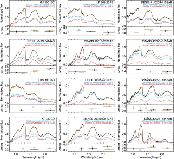
Figure 13. Integrated-light spectra (black) and best-matching component templates (colored lines) for binaries analyzed by our spectral decomposition method (see Section 5.2, Table 8). The bottom subpanels show the resolved photometry used to constrain the decomposition (filled black circles with errors) and the resulting flux ratios computed from the best-matching template pair (open brown squares). In some cases both HST/NICMOS medium-band and Keck photometry exist (e.g., 2MASS J0850+1057AB), and in one case there is no resolved photometry available (SDSS J0805+4812AB). For some binaries (e.g., 2MASS J0700+3157AB) we degrade our SpeX SXD spectra (R = 1200–2000) to the resolution of the prism template spectra (R = 120) and exclude the K band from the analysis.
Download figure:
Standard image High-resolution image
Figure 14. Same as Figure 13.
Download figure:
Standard image High-resolution image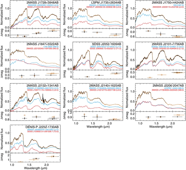
Figure 15. Same as Figure 13.
Download figure:
Standard image High-resolution imageTable 8. Component Spectral Types of Ultracool Binaries with Parallaxes
| Object | Primary | Secondary | Broadband | HST/NICMOS | Phot. |
|---|---|---|---|---|---|
| Type | Type | Data | Data | Ref. | |
| Derived from Our Template-matching Method | |||||
| GJ 1001BC | L5 ± 0.5 | L5 ± 0.5 | JHK | 110W, 170M | 1 |
| LP 349-25AB | M6.5 ± 1 | M8 ± 1 | JHK | ... | 5 |
| SDSSp J0423−0414AB | L6.5 ± 1 | T2 ± 0.5 | K | 110W, 170M | 1, 2 |
| 2MASS J0518−2828AB | L6 ± 1 | T4 ± 0.5 | ... | 110W, 170M | 1 |
| 2MASS J0700+3157AB | L3 ± 1 | L6.5 ± 1.5 | JHK | ... | 1 |
| LHS 1901AB | M7 ± 1 | M7 ± 1 | JHK | ... | 5 |
| SDSS J0805+4812AB | L4 ± 1 | T5 ± 0.5 | ... | ... | ... |
| 2MASS J0850+1057AB | L6.5 ± 1 | L8.5 ± 1 | JHK | 110W, 145M, 170M | 1, 3 |
| Gl 337CD | L8.5 ± 1 | L7.5 ± 2 | JHK | ... | 1 |
| 2MASS J0920+3517AB | L5.5 ± 1 | L9 ± 1.5 | JHK | ... | 1 |
| SDSS J0926+5847AB | T3.5 ± 1 | T5 ± 1 | ... | 110W, 170M | 1 |
| 2MASS J1017+1308AB | L1.5 ± 1 | L3 ± 1 | K | ... | 1 |
| SDSS J1021−0304AB | T0 ± 1 | T5 ± 0.5 | JHK | 110W, 170M | 1, 2 |
| Gl 417BC | L4.5 ± 1 | L6 ± 1 | K | ... | 1 |
| 2MASS J1146+2230AB | L3 ± 1 | L3 ± 1 | ... | ... | ... |
| 2MASS J1209−1004AB | T2.5 ± 0.5 | T6.5 ± 1 | JHKCH4s | ... | 10 |
| 2MASS J1225−2739AB | T5.5 ± 0.5 | T8 ± 0.5 | JHKCH4s | ... | 1 |
| DENIS-P J1228−1547AB | L5.5 ± 1 | L5.5 ± 1 | K | ... | 1 |
| Kelu-1AB | L2 ± 1 | L4 ± 1 | JHK | ... | 7 |
| 2MASS J1404−3159AB | L9 ± 1 | T5 ± 0.5 | JHK | ... | 1 |
| SDSS J1534+1615AB | T0 ± 1 | T5.5 ± 0.5 | JHK | ... | 8 |
| 2MASS J1534−2952AB | T4.5 ± 0.5 | T5 ± 0.5 | JHKCH4s | ... | 9 |
| 2MASS J1553+1532AB | T6.5 ± 0.5 | T7.5 ± 0.5 | JHKCH4s | 110W, 170M | 1, 2 |
| 2MASS J1728+3948AB | L5 ± 1 | L7 ± 1 | JHK | 110W, 145M, 170M | 1, 3 |
| LSPM J1735+2634AB | M7.5 ± 0.5 | L0 ± 1 | JHK | ... | 1 |
| 2MASS J1750+4424AB | M6.5 ± 1 | M8.5 ± 1 | JHK | ... | 6 |
| 2MASS J1847+5522AB | M6 ± 0.5 | M7 ± 0.5 | JHK | ... | 6 |
| SDSS J2052−1609AB | L8.5 ± 1.5 | T1.5 ± 0.5 | JHK | 110W, 170M | 1, 11 |
| 2MASS J2101+1756AB | L7 ± 1 | L8 ± 1 | K | ... | 6 |
| 2MASS J2132+1341AB | L4.5 ± 1.5 | L8.5 ± 1.5 | JHK | ... | 1 |
| 2MASS J2140+1625AB | M8 ± 0.5 | M9.5 ± 0.5 | JHK | ... | 6 |
| 2MASS J2206−2047AB | M8 ± 0.5 | M8 ± 0.5 | JHK | ... | 4 |
| DENIS-P J2252−1730AB | L4.5 ± 1.5 | T3.5 ± 1 | K | 110W, 170M | 1 |
| Published Values from Resolved Spectroscopy or Indices | |||||
| LHS 1070BC | M8.5 ± 0.5 | M9.5 ± 0.5 | ... | ... | A |
| 2MASS J0746+2000AB | L0 ± 0.5 | L1.5 ± 0.5 | ... | ... | B |
| HD 130948BC | L4 ± 1 | L4 ± 1 | ... | ... | C |
| Gl 569Bab | M8.5 ± 0.5 | M9.0 ± 0.5 | ... | ... | D |
| CFBDS J1458+1013AB | T9 ± 0.5 | >T10 | ... | ... | E |
| SCR J1845−6357AB | M8.5 ± 0.5 | T6 ± 0.5 | ... | ... | F |
 Ind Bab Ind Bab |
T1 ± 0.5 | T6 ± 0.5 | ... | ... | G |
| 2MASS J2234+4041AB | M6 ± 1 | M6 ± 1 | ... | ... | H |
Notes. We list component spectral types derived using the template-matching method described in Section 5.2 supplemented by spectral type determinations from the literature based on resolved spectroscopy or resolved photometric indices. The fourth and fifth columns list the MKO broadband and HST/NICMOS medium-band flux ratios used in the template matching, respectively. The last column gives references for the photometry used or for the source of the resolved spectroscopy. References. (1) This work (Tables 5 and 6); (2) Burgasser et al. 2006c; (3) Burgasser et al. 2010; (4) Dupuy et al. 2009a; (5) Dupuy et al. 2010; (6) Konopacky et al. 2010; (7) Liu & Leggett 2005; (8) Liu et al. 2006; (9) Liu et al. 2008; (10) Liu et al. 2010; (11) Stumpf et al. 2011. (A) Leinert et al. 2000; (B) Bouy et al. 2004; (C) Goto et al. 2002; (D) Lane et al. 2001; (E) Liu et al. 2011b; (F) Kasper et al. 2007; (G) King et al. 2010; (H) Allers et al. 2009.
Download table as: ASCIITypeset image
Finally, we note that there are several binaries with parallaxes for which we cannot derive component spectral types using this method, either because they do not have the needed spectral or photometric data or the data available do not sufficiently constrain the component types. Binaries with parallaxes for which we do not have spectra are 2MASS J0025+4759AB, HD 65216BC, LSPM J1314+1320AB, DENIS-P J1441−0945AB, and 2MASS J2331−0406AB. 2MASS J0856+2235AB, 2MASS J0952−1924AB, 2MASS J1239+5515AB, and LSR J1610−0040AB have no near-IR photometry. LHS 2397aAB has a spectrum and near-IR photometry, but the late-L companion is too faint to enable accurate spectral decomposition.
Our spectral decomposition analysis produces estimates of the flux ratios for bandpasses without resolved photometry. We synthesize flux ratios for every template pairing that agrees with the available resolved photometry (p value < 0.05). To determine the flux ratio and corresponding uncertainty in a given bandpass, we then use the weighted average and error given by the aforementioned Burgasser et al. (2010) weighting scheme. There are several cases that benefit from these flux ratios, in order of most to least reliable: (1) binaries with resolved KS photometry that we convert to MKO K (and vice versa, e.g., for ΔJMKO to ΔJ2MASS), (2) binaries with HST/NICMOS 0.9–1.8 μm photometry that we convert to JH photometry, (3) binaries with, e.g., only a K-band ratio for which we determine J and H flux ratios; and (4) one binary without any flux ratios (SDSS 0805+4812AB). In the following analysis we account for these differing levels of reliability when reporting absolute magnitudes and examining the location of binary components on CMDs.
5.3. Absolute Magnitudes of Single and Binary Objects
We combine our parallaxes with integrated-light photometry (and flux ratios in the case of binaries) to compute the absolute magnitudes for our sample. We have also compiled such measurements for all ultracool objects with published parallaxes. Table 9 presents a list of all ultracool dwarf parallax measurements, including objects that have parallax determinations by virtue of their companionship to stellar primaries. We compiled photometry from the literature for this entire sample, and for objects that have published photometry in only one system, (MKO or 2MASS) we use near-IR spectra, when available, to synthesize photometric conversions. For such objects we also synthesize Y − J colors to provide Y-band photometry when it is not measured directly. Using objects in the SpeX Prism Library with both 2MASS and MKO photometry we can test the quality of our synthetic photometric system offsets. The χ2 of our computed 2MASS/MKO offsets compared to measured values was 52.0 (98 dof), 96.6 (95 dof), and 51.4 (93 dof) for J, H, and K bands, respectively. Since χ2 is reasonable in all cases, we find that any systematic error in our computed offsets must be negligible compared to the uncertainty in the measured photometry (≲0.02 mag). However, when computing colors across different bandpasses we found an additional error of 0.05 mag was needed to explain the scatter in observed minus computed values. Thus, we treat synthesized photometric system offsets (e.g., JMKO − J2MASS) has having zero error, while we add 0.05 mag in quadrature to all synthesized Y − J photometry.
Table 9. All Ultracool Dwarfs with Parallaxes
| Object | αJ2000 | δJ2000 | Epoch | πabs | μαcos δ | μδ | μ | P.A. | Vtan | Ref. | Note |
|---|---|---|---|---|---|---|---|---|---|---|---|
| (deg) | (deg) | (MJD) | ('') | ('' yr−1) | ('' yr−1) | ('' yr−1) | (deg) | (km s−1) | |||
| SDSS J000013.54+255418.6 | 000.0564 | +25.9055 | 54301.63 | 0.0708(19) | −0.0191(14) | 0.1267(13) | 0.1281(13) | 351.4 ± 0.6 | 8.58 ± 0.24 | 1 | |
| LSR J0011+5908 | 002.8826 | +59.1445 | 51492.22 | 0.1083(14) | −0.8997 | −1.1654 | 1.4723 | 218 | 64 | 18 | |
| BRI 0021−0214 | 006.1027 | −01.9723 | 51071.24 | 0.0866(40) | −0.0804(38) | 0.1330(60) | 0.1550(70) | 328.8 ± 0.7 | 8.5 ± 0.5 | 26 | |
| LHS 1070A | 006.1841 | −27.1401 | 51542.05 | 0.1295(25) | −0.1330(50) | 0.6401(31) | 0.6537(30) | 348.3 ± 0.4 | 23.9 ± 0.5 | 6 | |
| PC 0025+0447 | 006.9249 | +05.0616 | 51768.41 | 0.0138(16) | 0.0105(4) | −0.0008(3) | 0.0105(4) | 94.6 ± 1.8 | 3.6 ± 0.5 | 8 | |
| LP 349-25AB | 006.9842 | +22.3255 | 54687.57 | 0.0696(9) | 0.4039(10) | −0.1654(15) | 0.4365(9) | 112.27 ± 0.21 | 29.7 ± 0.4 | 1 | Young? |
| 2MASSW J0030300−145033 | 007.6256 | −14.8426 | 51840.16 | 0.0374(45) | 0.2450(35) | −0.0282(18) | 0.2466(36) | 96.6 ± 0.4 | 31 ± 4 | 31 | |
| SDSSp J003259.36+141036.6 | 008.2474 | +14.1770 | 51878.20 | 0.0300(50) | 0.2730(70) | 0.0391(35) | 0.2760(70) | 81.8 ± 0.7 | 43 ± 8 | 31 | |
| ULAS J003402.77−005206.7 | 008.5116 | −00.8687 | 55051.60 | 0.0687(14) | −0.0167(10) | −0.3588(8) | 0.3592(8) | 182.66 ± 0.16 | 24.8 ± 0.5 | 1 | |
| 2MASSW J0036159+182110 | 009.0674 | +18.3529 | 51872.12 | 0.1142(8) | 0.8991(6) | 0.1200(16) | 0.9071(6) | 82.40 ± 0.10 | 37.66 ± 0.27 | 8 | |
| 2MASS J00501994−3322402 | 012.5873 | −33.3749 | 55050.57 | 0.0946(24) | 1.1506(21) | 0.9391(21) | 1.4851(21) | 50.78 ± 0.08 | 74.4 ± 1.9 | 1 | |
| RG 0050−2722 | 013.2279 | −27.0999 | 51128.04 | 0.0460(100) | 0.0562(48) | 0.0901(45) | 0.1063(45) | 32.0 ± 2.6 | 10.9 ± 2.5 | 27 | |
| CFBDS J005910.90−011401.3 | 014.7961 | −01.2336 | 55068.57 | 0.1032(21) | 0.8847(11) | 0.0440(12) | 0.8858(11) | 87.15 ± 0.08 | 40.7 ± 0.8 | 1 | |
| SDSSp J010752.33+004156.1 | 016.9684 | +00.6990 | 51789.23 | 0.0641(45) | 0.6280(70) | 0.0914(36) | 0.6350(70) | 81.7 ± 0.3 | 47 ± 3 | 31 | |
| CTI 012657.5+280202 | 021.9132 | +28.0982 | 50753.20 | 0.0305(5) | −0.1334(3) | −0.1348(3) | 0.1896(2) | 224.70 ± 0.10 | 29.5 ± 0.5 | 8 | |
| L 726-8AB | 024.7550 | −17.9507 | 51026.33 | 0.3750(40) | 3.2771(6) | 0.5908(6) | 3.3299(6) | 79.78 ± 0.01 | 42.1 ± 0.4 | 12 | |
| 2MASS J01490895+2956131 | 027.2873 | +29.9370 | 50755.30 | 0.0444(7) | 0.1757(8) | −0.4021(7) | 0.4388(7) | 156.40 ± 0.10 | 46.9 ± 0.7 | 8 | |
| SDSS J015141.69+124429.6 | 027.9232 | +12.7417 | 50704.37 | 0.0467(34) | 0.7418(42) | −0.0368(21) | 0.7427(42) | 92.84 ± 0.16 | 76 ± 5 | 31 | |
| DENIS-P J020529.0−115925AB | 031.3725 | −11.9916 | 51869.20 | 0.0506(15) | 0.4344(8) | 0.0549(8) | 0.4378(8) | 82.80 ± 0.10 | 41.0 ± 1.2 | 8 | Triple |
| SDSS J020742.48+000056.2 | 031.9285 | +00.0157 | 51774.32 | 0.0293(40) | 0.1588(31) | −0.0143(39) | 0.1595(30) | 95.1 ± 1.4 | 26 ± 4 | 20 | |
| 2MASSI J0243137−245329 | 040.8072 | −24.8916 | 51129.17 | 0.0936(36) | −0.2878(35) | −0.2076(29) | 0.3548(41) | 234.2 ± 0.3 | 18.0 ± 0.7 | 31 | |
| BRI B0246−1703 | 042.1708 | −16.8560 | 51026.38 | 0.0620(50) | 0.0210(90) | −0.2730(120) | 0.2740(120) | 175.7 ± 1.9 | 21.1 ± 2.1 | 27 | |
| TVLM 831-154910 | 042.5486 | −01.8582 | 51116.18 | 0.0302(45) | 0.0660(50) | −0.0559(44) | 0.0870(60) | 130.2 ± 1.2 | 13.6 ± 2.3 | 26 | |
| TVLM 831-161058 | 042.8053 | +00.7934 | 51788.42 | 0.0177(22) | 0.2340(70) | 0.0399(43) | 0.2380(70) | 80.3 ± 1.0 | 64 ± 8 | 26 | |
| TVLM 831-165166 | 042.9277 | −01.0350 | 51084.21 | 0.0195(39) | 0.4010(110) | 0.1970(70) | 0.4470(110) | 63.8 ± 0.7 | 109 ± 23 | 26 | |
| TVLM 832-10443 | 043.1095 | +00.9395 | 51789.29 | 0.0360(4) | −0.1752(2) | −0.1032(3) | 0.2033(1) | 239.50 ± 0.10 | 26.8 ± 0.3 | 8 | |
| Teegarden's star | 043.2535 | +16.8815 | 51486.22 | 0.2592(9) | 3.4228 | −3.8081 | 5.1203 | 138 | 94 | 11 | |
| PSO J043.5395+02.3995 | 043.5401 | +02.3997 | 55584.29 | 0.1710(450) | 2.5490(110) | 0.2310(110) | 2.5590(110) | 84.82 ± 0.25 | 71 ± 20 | 19 | |
| DENIS-P J0255.0−4700 | 043.7649 | −47.0142 | 51153.08 | 0.2014(39) | 0.9996(27) | −0.5655(37) | 1.1485(22) | 119.50 ± 0.20 | 27.0 ± 0.5 | 7 | |
| TVLM 832-42500 | 045.6455 | −01.2737 | 51084.34 | 0.0363(40) | 0.6720(190) | 0.3630(140) | 0.7640(210) | 61.6 ± 0.9 | 100 ± 12 | 26 | |
| LP 412-31 | 050.2486 | +18.9065 | 50747.41 | 0.0689(6) | 0.3493(5) | −0.2557(6) | 0.4329(3) | 126.20 ± 0.10 | 29.78 ± 0.26 | 8 | |
| 2MASSW J0326137+295015 | 051.5570 | +29.8376 | 50771.36 | 0.0310(15) | −0.0188(8) | 0.0668(8) | 0.0694(8) | 344.3 ± 0.7 | 10.6 ± 0.5 | 8 | |
| 2MASSI J0328426+230205 | 052.1777 | +23.0348 | 50748.33 | 0.0331(42) | 0.0126(26) | −0.0597(49) | 0.0610(49) | 168.1 ± 2.3 | 8.7 ± 1.4 | 31 | |
| LSPM J0330+5413 | 052.7038 | +54.2320 | 51172.21 | 0.1038(14) | −0.1510 | −0.0050 | 0.1511 | 268 | 7 | 18 | |
| LP 944-20 | 054.8967 | −35.4289 | 51154.22 | 0.2014(42) | 0.3240(80) | 0.2960(70) | 0.4390(80) | 47.6 ± 0.9 | 10.32 ± 0.29 | 27 | |
| 2MASP J0345432+254023 | 056.4299 | +25.6732 | 51530.21 | 0.0371(5) | −0.0960(3) | −0.0357(4) | 0.1024(3) | 249.60 ± 0.20 | 13.08 ± 0.18 | 8 | |
| LHS 1604 | 057.7502 | −00.8792 | 51828.37 | 0.0681(19) | 0.0086(11) | −0.4724(10) | 0.4725(10) | 178.96 ± 0.13 | 32.9 ± 0.9 | 21 | Overlum. |
| 2MASSI J0415195−093506 | 063.8381 | −09.5835 | 55070.64 | 0.1752(17) | 2.2143(12) | 0.5361(12) | 2.2782(12) | 76.39 ± 0.03 | 61.6 ± 0.6 | 1 | |
| SDSSp J042348.57−041403.5AB | 065.9517 | −04.2339 | 54341.64 | 0.0721(11) | −0.3276(5) | 0.0912(5) | 0.3401(5) | 285.56 ± 0.09 | 22.4 ± 0.3 | 1 | |
| LHS 191 | 066.5830 | +03.6100 | 51569.05 | 0.0584(18) | −0.1182(16) | −1.0154(17) | 1.0223(17) | 186.64 ± 0.09 | 83.0 ± 2.5 | 21 | |
| LHS 197 | 071.5771 | +48.7477 | 51545.16 | 0.0523(10) | 1.0258(7) | −0.6345(7) | 1.2062(7) | 121.74 ± 0.03 | 109.3 ± 2.1 | 21 | |
| LSR J0510+2713 | 077.5838 | +27.2342 | 50786.31 | 0.1007(16) | −0.2149 | −0.6339 | 0.6694 | 199 | 32 | 18 | |
| LHS 1742a | 077.6623 | +19.4022 | 50755.39 | 0.0134(10) | 0.7727(3) | −0.3075(3) | 0.8316(3) | 111.70 ± 0.02 | 294 ± 22 | 21 | Subdwarf |
| LSR J0515+5911 | 078.8789 | +59.1885 | 51197.13 | 0.0657(13) | 0.1127 | −1.0093 | 1.0156 | 174 | 73 | 18 | |
| 2MASS J05185995−2828372AB | 079.7498 | −28.4773 | 54366.66 | 0.0437(8) | −0.0700(5) | −0.2756(5) | 0.2844(5) | 194.25 ± 0.10 | 30.9 ± 0.6 | 1 | |
| 2MASS J05325346+8246465 | 083.2228 | +82.7796 | 51238.10 | 0.0423(18) | 2.0441(15) | −1.6654(15) | 2.6367(16) | 129.17 ± 0.03 | 296 ± 12 | 23 | Subdwarf |
| LHS 207 | 084.5527 | +79.5219 | 51822.51 | 0.0451(14) | 0.8412(6) | −0.8581(6) | 1.2016(6) | 135.57 ± 0.03 | 126 ± 4 | 21 | |
| SDSSp J053951.99−005902.0 | 084.9667 | −00.9839 | 51116.34 | 0.0761(22) | 0.1643(22) | 0.3159(32) | 0.3561(35) | 27.49 ± 0.28 | 22.2 ± 0.7 | 31 | |
| 2MASSI J0559191−140448 | 089.8314 | −14.0809 | 54519.25 | 0.0966(10) | 0.5718(16) | −0.3330(16) | 0.6617(16) | 120.21 ± 0.14 | 32.5 ± 0.3 | 1 | Overlum. |
| 2MASS J06411840−4322329 | 100.3267 | −43.3758 | 51271.04 | 0.0560(60) | 0.2160(90) | 0.6130(90) | 0.6490(90) | 19.4 ± 0.8 | 55 ± 6 | 2 | |
| 2MASS J07003664+3157266AB | 105.1533 | +31.9562 | 54513.30 | 0.0867(12) | 0.1424(7) | −0.5546(7) | 0.5726(7) | 165.60 ± 0.07 | 31.3 ± 0.4 | 1 | |
| ESO 207-61 | 106.9720 | −49.0140 | 51600.09 | 0.0541(45) | −0.0100(60) | 0.3910(70) | 0.3910(70) | 358.6 ± 0.8 | 34.3 ± 2.9 | 27 | |
| LHS 1901AB | 107.7987 | +43.4984 | 54513.31 | 0.0742(10) | 0.3544(9) | −0.5662(9) | 0.6680(9) | 147.96 ± 0.08 | 42.7 ± 0.6 | 1 | |
| 2MASS J07193188−5051410 | 109.8828 | −50.8614 | 51615.10 | 0.0326(24) | 0.1981(33) | −0.0614(38) | 0.2074(33) | 107.2 ± 1.1 | 30.2 ± 2.3 | 2 | |
| UGPS J072227.51−054031.2 | 110.6137 | −05.6750 | 55257.50 | 0.2428(24) | −0.9037(17) | 0.3518(14) | 0.9698(17) | 291.27 ± 0.08 | 18.94 ± 0.19 | 17 | |
| 2MASSI J0727182+171001 | 111.8297 | +17.1646 | 55125.63 | 0.1125(9) | 1.0471(9) | −0.7641(9) | 1.2962(9) | 126.12 ± 0.04 | 54.6 ± 0.4 | 1 | |
| LHS 234 | 115.0801 | −17.4125 | 50894.11 | 0.1070(16) | 1.1440(19) | −0.5530(27) | 1.2706(16) | 115.80 ± 0.13 | 56.3 ± 0.8 | 6 | |
| 2MASSI J0746425+200032AB | 116.6764 | +20.0089 | 54517.34 | 0.0811(9) | −0.3659(7) | −0.0527(5) | 0.3697(7) | 261.81 ± 0.08 | 21.61 ± 0.24 | 1 | |
| LP 423-31 | 118.0996 | +16.2044 | 50752.50 | 0.0544(10) | 0.1813 | −0.3562 | 0.3997 | 153 | 35 | 11 | |
| SDSS J080531.84+481233.0AB | 121.3814 | +48.2094 | 54428.60 | 0.0431(10) | −0.4583(7) | 0.0498(7) | 0.4610(7) | 276.20 ± 0.09 | 50.7 ± 1.2 | 1 | |
| DENIS J081730.0−615520 | 124.3750 | −61.9211 | 51545.24 | 0.2030(130) | −0.3300(500) | 1.0970(430) | 1.1470(420) | 343.0 ± 2.7 | 26.8 ± 2.0 | 3 | |
| 2MASSI J0825196+211552 | 126.3320 | +21.2645 | 50822.40 | 0.0938(10) | −0.5097(16) | −0.2884(19) | 0.5856(14) | 240.50 ± 0.20 | 29.6 ± 0.3 | 8 | |
| ULAS J082707.67−020408.2 | 126.7820 | −02.0689 | 53736.50 | 0.0260(31) | 0.0267(27) | −0.1089(24) | 0.1122(23) | 166.2 ± 1.4 | 20.5 ± 2.5 | 20 | |
| LHS 248 | 127.4562 | +26.7763 | 50846.25 | 0.2758(30) | −1.1390 | −0.6056 | 1.2900 | 242 | 22 | 29 | |
| SDSSp J083008.12+482847.4 | 127.5344 | +48.4801 | 51192.31 | 0.0764(34) | −1.0060(60) | −0.7698(48) | 1.2670(70) | 232.58 ± 0.15 | 79 ± 4 | 31 | |
| LHS 2021 | 127.6357 | +09.7876 | 51610.13 | 0.0598(45) | −0.5002(34) | −0.4487(36) | 0.6720(22) | 228.1 ± 0.4 | 53 ± 4 | 7 | |
| LHS 2026 | 128.1270 | −01.5772 | 51144.29 | 0.0508(6) | 0.1648(3) | −0.4691(3) | 0.4972(3) | 160.64 ± 0.03 | 46.4 ± 0.5 | 21 | |
| 2MASS J08354256−0819237 | 128.9274 | −08.3233 | 51201.24 | 0.1170(110) | −0.5200(90) | 0.2850(100) | 0.5930(80) | 298.8 ± 1.0 | 23.9 ± 2.3 | 2 | |
| SDSSp J083717.22−000018.3 | 129.3217 | −00.0050 | 51259.68 | 0.0340(130) | −0.0150(80) | −0.1720(170) | 0.1730(170) | 185.1 ± 2.8 | 24 ± 12 | 31 | |
| LHS 2034 | 130.1240 | +18.4026 | 51105.50 | 0.0713(11) | −0.8132(6) | −0.4480(6) | 0.9284(6) | 241.15 ± 0.04 | 61.7 ± 1.0 | 21 | |
| LHS 2065 | 133.4008 | −03.4923 | 51173.27 | 0.1173(15) | −0.5096(9) | −0.2004(10) | 0.5476(9) | 248.53 ± 0.10 | 22.13 ± 0.29 | 21 | |
| 2MASSI J0856479+223518AB | 134.1992 | +22.5884 | 54428.62 | 0.0324(10) | −0.1869(10) | −0.0132(8) | 0.1874(10) | 265.95 ± 0.24 | 27.4 ± 0.9 | 1 | |
| LP 368-128 | 135.0983 | +21.8348 | 51123.47 | 0.1569(27) | −0.5097(37) | −0.5823(34) | 0.7739(22) | 221.2 ± 0.3 | 23.4 ± 0.4 | 14 | |
| ULAS J090116.23−030635.0 | 135.3176 | −03.1097 | 53736.50 | 0.0626(26) | −0.0386(23) | −0.2612(28) | 0.2640(28) | 188.4 ± 0.5 | 20.0 ± 0.9 | 20 | |
| DENIS-P J0909.9−0658 | 137.4896 | −06.9718 | 51185.36 | 0.0425(42) | −0.1839(26) | 0.0207(30) | 0.1851(25) | 276.4 ± 0.9 | 20.6 ± 2.1 | 2 | |
| 2MASSW J0920122+351742AB | 140.0506 | +35.2949 | 54427.66 | 0.0344(8) | −0.1889(7) | −0.1985(7) | 0.2740(8) | 223.59 ± 0.13 | 37.8 ± 0.9 | 1 | |
| SDSS J092615.38+584720.9AB | 141.5642 | +58.7889 | 54513.41 | 0.0437(11) | 0.0102(5) | −0.2163(5) | 0.2165(5) | 177.30 ± 0.12 | 23.5 ± 0.6 | 1 | |
| 2MASSI J0937347+293142 | 144.3953 | +29.5281 | 51636.28 | 0.1634(18) | 0.9411(12) | −1.3155(12) | 1.6174(12) | 144.42 ± 0.04 | 46.9 ± 0.5 | 23 | Low-Z? |
| 2MASS J09393548−2448279 | 144.8979 | −24.8078 | 51584.13 | 0.1873(46) | 0.5734(23) | −1.0447(25) | 1.1917(25) | 151.24 ± 0.11 | 30.2 ± 0.7 | 5 | Low-Z? |
| TVLM 262-111511 | 145.5939 | +42.7599 | 50926.24 | 0.0340(60) | 0.1680(80) | −0.2000(90) | 0.2610(120) | 140.1 ± 0.5 | 36 ± 7 | 26 | |
| ULAS J094806.06+064805.0 | 147.0252 | +06.8014 | 53736.50 | 0.0272(42) | 0.1990(70) | −0.2740(70) | 0.3390(70) | 143.9 ± 1.1 | 59 ± 9 | 20 | |
| TVLM 262-70502 | 147.9487 | +42.5641 | 50931.23 | 0.0256(40) | 0.0969(47) | −0.1760(70) | 0.2010(80) | 151.2 ± 0.9 | 37 ± 6 | 26 | |
| 2MASS J09522188−1924319AB | 148.0912 | −19.4089 | 50931.11 | 0.0338(30) | −0.0611(35) | −0.1016(28) | 0.1186(21) | 211.0 ± 1.9 | 16.6 ± 1.5 | 7 | |
| 2MASS J10043929−3335189 | 151.1637 | −33.5886 | 51300.99 | 0.0550(60) | 0.2435(37) | −0.2533(37) | 0.3514(37) | 136.1 ± 0.6 | 30 ± 3 | 2 | |
| TVLM 263-71765 | 152.7510 | +42.7510 | 51230.33 | 0.0319(29) | −0.1330(60) | −0.1490(60) | 0.2000(70) | 221.8 ± 1.4 | 29.8 ± 2.9 | 26 | |
| SSSPM J1013−1356 | 153.2806 | −13.9390 | 51214.24 | 0.0203(20) | 0.0691(13) | −1.0249(13) | 1.0272(13) | 176.14 ± 0.07 | 240 ± 23 | 23 | Subdwarf |
| 2MASSI J1017075+130839AB | 154.2818 | +13.1442 | 54514.44 | 0.0302(14) | 0.0479(5) | −0.1178(5) | 0.1272(5) | 157.86 ± 0.24 | 20.0 ± 0.9 | 1 | |
| ULAS J101821.78+072547.1 | 154.5908 | +07.4298 | 53736.50 | 0.0250(20) | −0.1837(26) | −0.0151(31) | 0.1843(26) | 265.3 ± 1.0 | 34.9 ± 2.9 | 20 | |
| 2MASS J10185879−2909535 | 154.7450 | −29.1649 | 51243.10 | 0.0353(32) | −0.3401(20) | −0.0939(26) | 0.3529(19) | 254.6 ± 0.4 | 47 ± 4 | 2 | |
| SDSS J102109.69−030420.1AB | 155.2902 | −03.0723 | 54514.45 | 0.0299(13) | −0.1626(6) | −0.0745(7) | 0.1789(6) | 245.38 ± 0.21 | 28.3 ± 1.3 | 1 | |
| TVLM 213-2005 | 155.3643 | +50.9179 | 51175.45 | 0.0301(4) | −0.3856(1) | 0.0514(7) | 0.3890(1) | 277.60 ± 0.10 | 61.3 ± 0.8 | 8 | |
| 2MASSI J1047538+212423 | 161.9744 | +21.4065 | 50842.42 | 0.0947(38) | −1.6620(70) | −0.4741(42) | 1.7280(80) | 254.08 ± 0.13 | 87 ± 4 | 31 | |
| LHS 292 | 162.0524 | −11.3356 | 51203.31 | 0.2203(36) | 0.6162 | −1.5252 | 1.6450 | 158 | 35 | 29 | |
| LHS 2314 | 162.2641 | +05.0396 | 51586.21 | 0.0411(23) | −0.3651(15) | −0.4623(15) | 0.5891(14) | 218.30 ± 0.15 | 68 ± 4 | 21 | |
| Wolf 359 | 164.1203 | +07.0147 | 51604.20 | 0.4191(21) | −3.8467 | −2.6935 | 4.6960 | 235 | 53 | 29 | |
| DENIS-P J1058.7−1548 | 164.6995 | −15.8048 | 50897.23 | 0.0577(10) | −0.2529(5) | 0.0414(4) | 0.2563(5) | 279.30 ± 0.10 | 21.1 ± 0.4 | 8 | |
| SSSPM J1102−3431 | 165.5410 | −34.5099 | 51264.16 | 0.0181(5) | −0.0671(6) | −0.0140(6) | 0.0686(6) | 258.2 ± 0.5 | 18.0 ± 0.5 | 25 | TWA |
| LHS 2351 | 166.5791 | +04.4758 | 51589.22 | 0.0481(31) | −0.3290(90) | 0.3720(90) | 0.4970(120) | 318.5 ± 0.6 | 49 ± 3 | 27 | |
| SDSS J111010.01+011613.1 | 167.5412 | +01.2700 | 54514.50 | 0.0521(12) | −0.2171(7) | −0.2809(7) | 0.3550(7) | 217.71 ± 0.11 | 32.3 ± 0.7 | 1 | |
| 2MASS J11145133−2618235 | 168.7033 | −26.3075 | 55280.39 | 0.1792(14) | −3.0189(11) | −0.3840(16) | 3.0432(11) | 262.75 ± 0.03 | 80.5 ± 0.6 | 1 | |
| LHS 2397aAB | 170.4539 | −13.2190 | 54520.49 | 0.0730(21) | −0.4869(23) | −0.0614(18) | 0.4908(23) | 262.81 ± 0.21 | 31.9 ± 0.9 | 1 | |
| 2MASSW J1146345+223053AB | 176.6441 | +22.5152 | 54514.51 | 0.0349(10) | 0.0256(7) | 0.0894(8) | 0.0930(8) | 16.0 ± 0.4 | 12.6 ± 0.4 | 1 | |
| ULAS J115038.79+094942.9 | 177.6616 | +09.8286 | 53736.50 | 0.0170(80) | −0.1070(160) | −0.0320(80) | 0.1120(160) | 253 ± 4 | 32 ± 19 | 20 | |
| LHS 2471 | 178.4695 | +06.9989 | 51607.32 | 0.0703(27) | 0.2572(19) | −0.8536(18) | 0.8915(18) | 163.23 ± 0.12 | 60.2 ± 2.3 | 21 | |
| 2MASSW J1207334−393254b | 181.8894 | −39.5483 | 51300.18 | 0.0191(4) | −0.0642(4) | −0.0226(4) | 0.0681(4) | 250.6 ± 0.3 | 16.9 ± 0.4 | 10 | TWA, planet |
| 2MASSW J1207334−393254 | 181.8894 | −39.5483 | 51300.18 | 0.0191(4) | −0.0642(4) | −0.0226(4) | 0.0681(4) | 250.6 ± 0.3 | 16.9 ± 0.4 | 10 | TWA |
| 2MASS J12095613−1004008AB | 182.4851 | −10.0679 | 54513.52 | 0.0458(10) | 0.2661(5) | −0.3554(6) | 0.4440(6) | 143.18 ± 0.06 | 46.0 ± 1.0 | 1 | |
| 2MASSI J1217110−031113 | 184.2963 | −03.1870 | 51208.26 | 0.0908(22) | −1.0544(17) | 0.0756(18) | 1.0571(17) | 274.10 ± 0.10 | 55.2 ± 1.3 | 28 | |
| BRI B1222−1222 | 186.2176 | −12.6431 | 50903.27 | 0.0586(38) | −0.2610(110) | −0.1870(110) | 0.3220(110) | 234.4 ± 1.9 | 26.0 ± 1.9 | 27 | |
| 2MASS J12255432−2739466AB | 186.4763 | −27.6630 | 50998.97 | 0.0751(25) | 0.3849(19) | −0.6282(26) | 0.7368(29) | 148.50 ± 0.10 | 46.5 ± 1.6 | 28 | |
| DENIS-P J1228.2−1547AB | 187.0639 | −15.7935 | 54514.54 | 0.0448(18) | 0.1344(9) | −0.1853(9) | 0.2289(9) | 144.04 ± 0.22 | 24.2 ± 1.0 | 1 | |
| 2MASS J12373919+6526148 | 189.4133 | +65.4374 | 51250.47 | 0.0961(48) | −1.0020(80) | −0.5250(60) | 1.1310(90) | 242.33 ± 0.23 | 55.9 ± 2.9 | 31 | |
| 2MASSW J1239272+551537AB | 189.8645 | +55.2605 | 54513.53 | 0.0424(21) | 0.1252(11) | −0.0004(10) | 0.1252(11) | 90.2 ± 0.5 | 14.0 ± 0.7 | 1 | |
| SDSSp J125453.90−012247.4 | 193.7247 | −01.3799 | 51202.38 | 0.0849(19) | −0.4787(20) | 0.1301(34) | 0.4961(18) | 285.2 ± 0.4 | 27.7 ± 0.6 | 8 | |
| SSSPM J1256−1408 | 194.0586 | −14.1443 | 51238.21 | 0.0188(19) | −0.7399(13) | −1.0006(14) | 1.2445(14) | 216.48 ± 0.06 | 314 ± 31 | 23 | Subdwarf |
| SDSS J125637.13−022452.4 | 194.1549 | −02.4145 | 51220.27 | 0.0111(29) | −0.5121(19) | −0.2977(19) | 0.5923(19) | 239.83 ± 0.18 | 254 ± 70 | 23 | Subdwarf |
| Kelu-1AB | 196.4168 | −25.6848 | 54514.56 | 0.0497(24) | −0.2992(12) | −0.0041(15) | 0.2992(12) | 269.21 ± 0.28 | 28.5 ± 1.4 | 1 | |
| LSPM J1314+1320AB | 198.5850 | +13.3337 | 51573.43 | 0.0610(28) | −0.2424 | −0.1856 | 0.3053 | 233 | 24 | 18 | |
| ULAS J131508.42+082627.4 | 198.7851 | +08.4409 | 53736.50 | 0.0430(80) | −0.0600(90) | −0.0960(90) | 0.1130(100) | 212 ± 4 | 12.6 ± 2.6 | 20 | |
| SDSSp J132629.82−003831.5 | 201.6242 | −00.6421 | 51212.34 | 0.0500(60) | −0.2260(80) | −0.1070(60) | 0.2510(90) | 244.6 ± 1.0 | 24 ± 3 | 31 | |
| 2MASSW J1328550+211449 | 202.2293 | +21.2468 | 51321.15 | 0.0310(38) | 0.2192(17) | −0.4282(18) | 0.4811(18) | 152.90 ± 0.20 | 74 ± 9 | 8 | |
| ULAS J133553.45+113005.2 | 203.9728 | +11.5014 | 55287.48 | 0.0999(16) | −0.1908(14) | −0.2024(14) | 0.2782(12) | 223.3 ± 0.3 | 13.20 ± 0.22 | 1 | |
| SDSSp J134646.45−003150.4 | 206.6931 | −00.5306 | 51943.33 | 0.0683(23) | −0.5032(32) | −0.1143(19) | 0.5160(33) | 257.20 ± 0.20 | 35.8 ± 1.2 | 28 | |
| 2MASS J14044948−3159330AB | 211.2071 | −31.9924 | 54515.60 | 0.0421(11) | 0.3448(10) | −0.0108(14) | 0.3450(10) | 91.79 ± 0.23 | 38.8 ± 1.0 | 1 | |
| SDSS J141624.08+134826.7 | 214.1009 | +13.8080 | 55307.42 | 0.1097(13) | 0.0952(14) | 0.1329(14) | 0.1635(14) | 35.6 ± 0.5 | 7.07 ± 0.10 | 1 | Low-Z? |
| LSR J1425+7102 | 216.2713 | +71.0360 | 51318.21 | 0.0134(5) | −0.6050(3) | −0.1599(10) | 0.6258(2) | 255.20 ± 0.10 | 222 ± 9 | 9 | Subdwarf |
| LHS 2919 | 217.0175 | +13.9372 | 51227.42 | 0.0828(41) | −0.3584 | −0.4742 | 0.5944 | 217 | 34 | 18 | |
| LHS 2924 | 217.1801 | +33.1775 | 51612.34 | 0.0908(13) | −0.3457(4) | −0.7079(4) | 0.7878(4) | 206.03 ± 0.03 | 41.1 ± 0.6 | 21 | |
| LHS 2930 | 217.6578 | +59.7236 | 51251.47 | 0.1038(14) | −0.8025(7) | 0.1668(6) | 0.8197(7) | 281.74 ± 0.04 | 37.4 ± 0.5 | 21 | |
| SDSS J143517.20−004612.9 | 218.8217 | −00.7703 | 51285.21 | 0.0100(50) | 0.0220(80) | 0.0100(60) | 0.0250(90) | 65 ± 11 | 12 ± 10 | 31 | |
| SDSS J143535.72−004347.0 | 218.8989 | −00.7298 | 51285.21 | 0.0160(60) | 0.0218(46) | −0.1050(90) | 0.1080(90) | 168.3 ± 2.3 | 32 ± 13 | 31 | |
| LHS 377 | 219.7513 | +18.6607 | 51614.38 | 0.0284(8) | −0.0115(2) | −1.2158(3) | 1.2159(3) | 180.54 ± 0.01 | 203 ± 6 | 21 | Subdwarf |
| 2MASSW J1439284+192915 | 219.8682 | +19.4875 | 50609.26 | 0.0696(5) | −1.2298(7) | 0.4067(22) | 1.2953(2) | 288.30 ± 0.10 | 88.2 ± 0.6 | 8 | |
| SSSPM J1444−2019 | 221.0861 | −20.3229 | 50941.14 | 0.0617(21) | −2.8939(25) | −1.9549(25) | 3.4924(25) | 235.96 ± 0.04 | 268 ± 9 | 23 | Subdwarf |
| SDSSp J144600.60+002452.0 | 221.5026 | +00.4144 | 51641.24 | 0.0455(33) | 0.1800(70) | −0.0655(41) | 0.1910(70) | 110.1 ± 1.0 | 20.0 ± 1.6 | 31 | |
| LHS 3003 | 224.1596 | −28.1632 | 50990.95 | 0.1590(50) | −0.4700(100) | −0.8440(120) | 0.9660(130) | 209.1 ± 0.5 | 28.7 ± 1.0 | 27 | |
| CFBDS J145829+10134AB | 224.6225 | +10.2284 | 55283.56 | 0.0313(25) | 0.1740(21) | −0.3818(25) | 0.4196(26) | 155.50 ± 0.28 | 63 ± 5 | 1 | |
| TVLM 513-46546 | 225.2841 | +22.8339 | 51613.40 | 0.0944(6) | −0.0246(3) | −0.0579(4) | 0.0629(4) | 203.0 ± 0.3 | 3.16 ± 0.03 | 8 | |
| TVLM 513-42404 | 225.5888 | +25.4319 | 51320.26 | 0.0350(100) | −0.1210(90) | −0.0380(70) | 0.1270(90) | 253 ± 3 | 17 ± 5 | 26 | |
| 2MASSW J1503196+252519 | 225.8321 | +25.4237 | 54575.47 | 0.1572(22) | 0.0901(16) | 0.5618(16) | 0.5690(16) | 9.11 ± 0.16 | 17.16 ± 0.25 | 1 | |
| SDSS J150411.63+102718.3 | 226.0493 | +10.4546 | 55050.24 | 0.0461(15) | 0.3737(19) | −0.3692(20) | 0.5253(19) | 134.66 ± 0.22 | 54.0 ± 1.7 | 1 | Overlum. |
| 2MASSW J1507476−162738 | 226.9487 | −16.4607 | 50936.22 | 0.1364(6) | −0.1615(15) | −0.8885(6) | 0.9031(5) | 190.30 ± 0.10 | 31.39 ± 0.14 | 8 | |
| TVLM 868-110639 | 227.5702 | −02.6855 | 51257.27 | 0.0612(47) | −0.4050(120) | 0.0240(60) | 0.4060(120) | 273.4 ± 0.8 | 31.5 ± 2.6 | 26 | |
| TVLM 513-8328 | 228.5856 | +23.6848 | 50613.29 | 0.0241(45) | −0.1130(80) | −0.0480(70) | 0.1230(90) | 247 ± 3 | 24 ± 5 | 26 | |
| SDSS J153417.05+161546.1AB | 233.5711 | +16.2630 | 54515.65 | 0.0249(11) | −0.0799(7) | −0.0361(8) | 0.0877(7) | 245.7 ± 0.5 | 16.7 ± 0.8 | 1 | |
| 2MASSI J1534498−295227AB | 233.7083 | −29.8747 | 54515.66 | 0.0624(13) | 0.0934(10) | −0.2600(13) | 0.2763(13) | 160.24 ± 0.20 | 21.0 ± 0.4 | 1 | |
| DENIS-P J153941.9−052042 | 234.9246 | −05.3452 | 51256.33 | 0.0645(34) | 0.6013(27) | 0.1047(34) | 0.6104(26) | 80.1 ± 0.3 | 44.9 ± 2.4 | 2 | |
| WISEPA J154151.66−225025.2 | 235.4649 | −22.8405 | 55665.00 | 0.3500(1100) | −0.7800(2300) | −0.2100(2600) | 0.8500(2300) | 254 ± 18 | 11 ± 5 | 16 | |
| 2MASS J15462718−3325111 | 236.6133 | −33.4198 | 51003.16 | 0.0880(19) | 0.1211(23) | 0.1901(23) | 0.2254(22) | 32.5 ± 0.6 | 12.15 ± 0.29 | 28 | |
| 2MASSW J1553022+153236AB | 238.2585 | +15.5442 | 54576.51 | 0.0751(9) | −0.3858(7) | 0.1662(8) | 0.4201(7) | 293.30 ± 0.12 | 26.5 ± 0.3 | 1 | |
| LSR J1610−0040AB | 242.6208 | −00.6814 | 51243.36 | 0.0310(3) | −0.7942(21) | −1.2090(14) | 1.4465(2) | 213.30 ± 0.10 | 221.0 ± 1.8 | 9 | Subdwarf |
| SDSSp J162414.37+002915.6 | 246.0599 | +00.4877 | 51290.23 | 0.0909(12) | −0.3728(16) | −0.0091(19) | 0.3730(16) | 268.6 ± 0.3 | 19.45 ± 0.27 | 28 | |
| 2MASS J16262034+3925190 | 246.5848 | +39.4220 | 50932.43 | 0.0299(11) | −1.3815(10) | 0.2394(10) | 1.4021(10) | 279.83 ± 0.04 | 223 ± 8 | 23 | Subdwarf |
| SDSS J162838.77+230821.1 | 247.1624 | +23.1388 | 54576.52 | 0.0751(9) | 0.4123(8) | −0.4430(8) | 0.6052(8) | 137.06 ± 0.07 | 38.2 ± 0.5 | 1 | |
| 2MASSW J1632291+190441 | 248.1213 | +19.0780 | 50607.36 | 0.0656(21) | 0.2931(9) | −0.0538(10) | 0.2980(9) | 100.40 ± 0.20 | 21.5 ± 0.7 | 8 | |
| LHS 3241 | 251.6315 | +34.5821 | 51316.27 | 0.0843(8) | −0.3690 | −0.3945 | 0.5402 | 223 | 30 | 11 | |
| WISE J164715.57+563208.3 | 251.8159 | +56.5349 | 51308.41 | 0.1160(290) | −0.1660(90) | 0.2420(80) | 0.2940(80) | 325.6 ± 1.7 | 12 ± 3 | 16 | Very red |
| 2MASSW J1658037+702701 | 254.5159 | +70.4504 | 51626.38 | 0.0539(7) | −0.1468(7) | −0.3133(9) | 0.3460(9) | 205.10 ± 0.10 | 30.4 ± 0.4 | 8 | |
| DENIS-P J170548.3−051645 | 256.4514 | −05.2795 | 51268.32 | 0.0450(120) | 0.1110(100) | −0.1150(100) | 0.1600(100) | 136 ± 4 | 17 ± 5 | 2 | |
| 2MASSI J1711457+223204 | 257.9406 | +22.5346 | 50614.33 | 0.0331(48) | 0.0310(70) | −0.0042(39) | 0.0310(80) | 98 ± 7 | 4.5 ± 1.3 | 31 | |
| 2MASSW J1728114+394859AB | 262.0481 | +39.8164 | 54576.59 | 0.0387(7) | 0.0358(5) | −0.0183(5) | 0.0402(5) | 117.2 ± 0.8 | 4.92 ± 0.11 | 1 | |
| LSPM J1735+2634AB | 263.8045 | +26.5793 | 54576.60 | 0.0667(14) | 0.1496(7) | −0.3192(8) | 0.3525(8) | 154.88 ± 0.12 | 25.1 ± 0.5 | 1 | |
| WISEP J174124.27+255319.6 | 265.3526 | +25.8929 | 51645.39 | 0.1820(380) | −0.4880(160) | −1.4760(160) | 1.5550(160) | 198.3 ± 0.6 | 41 ± 9 | 16 | |
| 2MASSW J1750129+442404AB | 267.5533 | +44.4019 | 54576.60 | 0.0303(10) | −0.0151(8) | 0.1433(9) | 0.1441(9) | 354.0 ± 0.3 | 22.6 ± 0.7 | 1 | |
| 2MASS J17502484−0016151 | 267.6035 | −00.2709 | 51257.41 | 0.1085(26) | −0.3992(32) | 0.1957(33) | 0.4445(32) | 296.1 ± 0.4 | 19.4 ± 0.5 | 2 | |
| SDSSp J175032.96+175903.9 | 267.6372 | +17.9845 | 51260.48 | 0.0362(45) | 0.1780(70) | 0.1000(50) | 0.2040(80) | 60.8 ± 1.1 | 27 ± 4 | 31 | |
| LP 44-162 | 269.3142 | +70.7003 | 51316.33 | 0.0524(11) | 0.0130 | 0.3292 | 0.3295 | 2 | 30 | 18 | |
| 2MASSI J1835379+325954 | 278.9079 | +32.9985 | 50923.48 | 0.1765(5) | −0.0807(13) | −0.7547(11) | 0.7590(11) | 186.10 ± 0.10 | 20.39 ± 0.06 | 22 | |
| LP 335-12 | 279.8879 | +29.8712 | 51638.45 | 0.0793(20) | 0.0798 | −0.2183 | 0.2324 | 160 | 14 | 18 | |
| LP 44-334 | 280.0099 | +72.6817 | 51319.46 | 0.0593(22) | −0.0330 | 0.1891 | 0.1920 | 350 | 15 | 18 | |
| 2MASSW J1841086+311727 | 280.2859 | +31.2911 | 50924.44 | 0.0236(19) | 0.0594(32) | 0.0416(26) | 0.0726(37) | 55.0 ± 1.5 | 14.6 ± 1.4 | 31 | |
| CE 507 | 280.8016 | −33.3754 | 51620.40 | 0.0655(25) | −0.1557(42) | −0.3615(28) | 0.3936(24) | 203.3 ± 0.7 | 28.5 ± 1.1 | 7 | |
| LHS 3406 | 280.8422 | +40.6725 | 51288.50 | 0.0707(8) | −0.1187(4) | 0.5940(4) | 0.6057(4) | 348.70 ± 0.04 | 40.6 ± 0.5 | 21 | Overlum. |
| SCR J1845−6357AB | 281.2726 | −63.9632 | 51693.19 | 0.2595(11) | 2.5919(18) | 0.6175(27) | 2.6644(17) | 76.60 ± 0.06 | 48.69 ± 0.21 | 14 | |
| 2MASSI J1847034+552243AB | 281.7648 | +55.3788 | 54314.36 | 0.0298(11) | 0.1244(10) | −0.0621(11) | 0.1391(10) | 116.5 ± 0.5 | 22.1 ± 0.8 | 1 | |
| LSR J2036+5059 | 309.0902 | +51.0014 | 51702.31 | 0.0216(13) | 0.7552(13) | 1.2578(13) | 1.4671(13) | 30.98 ± 0.05 | 322 ± 19 | 23 | Subdwarf |
| SDSS J205235.31−160929.8AB | 313.1477 | −16.1580 | 54314.45 | 0.0339(8) | 0.3997(6) | 0.1527(7) | 0.4279(6) | 69.09 ± 0.09 | 59.8 ± 1.4 | 1 | |
| 2MASS J21011544+1756586AB | 315.3143 | +17.9496 | 51671.49 | 0.0301(34) | 0.1440(29) | −0.1509(30) | 0.2085(37) | 136.3 ± 0.5 | 33 ± 4 | 31 | |
| LP 397-10 | 319.0262 | +22.6462 | 51004.42 | 0.0484(11) | 0.0680 | 0.1789 | 0.1914 | 21 | 19 | 11 | |
| [HB88] M18 | 319.6323 | −45.0979 | 51437.04 | 0.0470(80) | 0.4090(70) | −0.4700(80) | 0.6230(90) | 139.0 ± 0.5 | 63 ± 11 | 27 | |
| LSPM J2124+4003 | 321.1348 | +40.0667 | 51689.39 | 0.0667(13) | 0.5441 | 0.4455 | 0.7032 | 51 | 50 | 11 | |
| HB 2124−4228 | 321.8589 | −42.2551 | 51410.09 | 0.0290(60) | 0.1280(70) | −0.1140(60) | 0.1720(90) | 131.8 ± 0.7 | 28 ± 6 | 27 | |
| [HB88] M20 | 322.5359 | −44.7744 | 51410.11 | 0.0370(160) | 0.0630(60) | −0.4370(80) | 0.4410(80) | 171.8 ± 0.7 | 56 ± 29 | 27 | |
| 2MASSI J2132114+134158AB | 323.0480 | +13.6995 | 54314.50 | 0.0360(7) | 0.0194(14) | −0.1225(7) | 0.1240(7) | 171.0 ± 0.6 | 16.3 ± 0.3 | 1 | |
| 2MASSW J2140293+162518AB | 325.1220 | +16.4217 | 54314.49 | 0.0325(11) | −0.0686(8) | −0.0828(8) | 0.1075(8) | 219.6 ± 0.4 | 15.7 ± 0.5 | 1 | |
| LSPM J2158+6117 | 329.6441 | +61.2850 | 51448.32 | 0.0592(22) | 0.7923 | 0.1061 | 0.7993 | 82 | 64 | 11 | |
| 2MASSW J2206228−204705AB | 331.5952 | −20.7847 | 54635.61 | 0.0357(12) | 0.0130(9) | −0.0319(11) | 0.0344(11) | 157.8 ± 1.5 | 4.57 ± 0.21 | 1 | |
| GRH 2208−20 | 332.7083 | −19.8736 | 50998.35 | 0.0247(5) | −0.2068(11) | −0.6600(4) | 0.6917(2) | 197.40 ± 0.10 | 132.7 ± 2.7 | 8 | |
| TVLM 890-60235 | 335.7731 | +00.5030 | 51742.31 | 0.0194(22) | −0.0706(16) | −0.0165(28) | 0.0725(15) | 256.9 ± 2.2 | 17.7 ± 2.1 | 26 | |
| 2MASSW J2224438−015852 | 336.1839 | −01.9830 | 54316.47 | 0.0862(11) | 0.4686(5) | −0.8648(6) | 0.9836(6) | 151.55 ± 0.03 | 54.1 ± 0.7 | 1 | Very red |
| LHS 523 | 337.2267 | −13.4216 | 50989.35 | 0.0888(49) | −0.3166 | −1.0357 | 1.0830 | 197 | 58 | 29 | |
| 2MASS J22344161+4041387AB | 338.6734 | +40.6941 | 51096.09 | 0.0031(6) | −0.0017(5) | −0.0031(5) | 0.0035(5) | 209 ± 8 | 5.4 ± 1.2 | 30 | LkHα 233 |
| LP 460-44 | 338.9544 | +18.6750 | 50725.17 | 0.0435(36) | 0.3234 | 0.0423 | 0.3262 | 83 | 36 | 11 | |
| ULAS J223955.76+003252.6 | 339.9823 | +00.5479 | 53736.50 | 0.0100(50) | 0.1250(50) | −0.1080(50) | 0.1660(50) | 130.9 ± 1.8 | 75 ± 50 | 20 | |
| DENIS-P J225210.73−173013.4AB | 343.0458 | −17.5031 | 54318.51 | 0.0632(16) | 0.3972(23) | 0.1443(36) | 0.4226(20) | 70.0 ± 0.5 | 31.7 ± 0.8 | 1 | |
| SDSSp J225529.09−003433.4 | 343.8711 | −00.5760 | 51393.27 | 0.0162(26) | −0.0362(14) | −0.1763(25) | 0.1799(26) | 191.6 ± 0.4 | 53 ± 9 | 31 | |
| 2MASS J23062928−0502285 | 346.6220 | −05.0413 | 51075.18 | 0.0826(26) | 0.9221(22) | −0.4719(32) | 1.0358(18) | 117.10 ± 0.19 | 59.4 ± 1.9 | 7 | |
| APMPM J2330−4737 | 352.5672 | −47.6128 | 51834.07 | 0.0727(33) | −0.5648(46) | −0.9741(34) | 1.1261(26) | 210.10 ± 0.26 | 73 ± 3 | 7 | |
| APMPM J2331−2750 | 352.8406 | −27.8306 | 51341.43 | 0.0691(21) | 0.0772(20) | 0.7598(13) | 0.7637(13) | 5.80 ± 0.15 | 52.4 ± 1.6 | 7 | |
| APMPM J2344−2906 | 355.8833 | −29.1076 | 51126.01 | 0.0323(46) | 0.3412(39) | −0.2233(48) | 0.4077(29) | 123.2 ± 0.8 | 60 ± 9 | 7 | |
| 2MASSI J2356547−155310 | 359.2282 | −15.8864 | 51011.33 | 0.0690(34) | −0.4434(21) | −0.6002(25) | 0.7462(29) | 216.46 ± 0.11 | 51.2 ± 2.5 | 31 | |
| APMPM J2359−6246 | 359.6786 | −62.7618 | 51526.09 | 0.0480(22) | 0.5728(25) | 0.0836(38) | 0.5789(25) | 81.7 ± 0.4 | 57.3 ± 2.7 | 7 | |
| Ultracool Companions | |||||||||||
| 2MASSI J0003422−282241 | 000.9277 | −28.3783 | 55050.53 | 0.0257(9) | 0.2808(9) | −0.1415(8) | 0.3145(10) | 116.75 ± 0.13 | 58.0 ± 2.1 | 30 | Overlum. |
| GJ 1001BC | 001.1452 | −40.7350 | 51392.29 | 0.0769(40) | 0.6436(32) | −1.4943(21) | 1.6270(18) | 156.70 ± 0.12 | 100 ± 5 | 14 | |
| HD 1160B | 003.9887 | +04.2511 | 51872.27 | 0.0097(5) | 0.0211(5) | −0.0142(4) | 0.0255(5) | 123.9 ± 0.9 | 12.5 ± 0.6 | 30 | Young |
| LHS 1070BC | 006.1841 | −27.1401 | 51542.05 | 0.1295(25) | −0.1325(49) | 0.6401(31) | 0.6537(30) | 348.3 ± 0.4 | 23.9 ± 0.5 | 6 | |
| 2MASS J00250365+4759191AB | 006.2652 | +47.9887 | 51123.26 | 0.0228(9) | 0.2750(7) | 0.0117(8) | 0.2752(7) | 87.57 ± 0.16 | 57.2 ± 2.2 | 30 | |
| HD 3651B | 009.8291 | +21.2548 | 50726.24 | 0.0904(3) | −0.4607(3) | −0.3695(3) | 0.5905(3) | 231.27 ± 0.03 | 30.96 ± 0.11 | 30 | |
| GJ 1048B | 038.9997 | −23.5224 | 51128.19 | 0.0470(9) | 0.0836(10) | 0.0136(8) | 0.0848(10) | 80.8 ± 0.5 | 8.55 ± 0.20 | 30 | |
| β Pic b | 086.8212 | −51.0665 | 51518.17 | 0.0514(1) | 0.0046(1) | 0.0831(2) | 0.0832(2) | 3.20 ± 0.08 | 7.67 ± 0.02 | 30 | β Pic, planet |
| CD-35 2722 B | 092.3301 | −35.8253 | 51470.29 | 0.0470(30) | −0.0085(47) | −0.0615(41) | 0.0622(41) | 188 ± 4 | 6.3 ± 0.6 | 32 | AB Dor |
| Gl 229B | 092.6443 | −21.8645 | 51191.20 | 0.1738(10) | −0.1371(5) | −0.7142(8) | 0.7272(8) | 190.87 ± 0.04 | 19.83 ± 0.12 | 30 | |
| AB Pic b | 094.8038 | −58.0543 | 51506.26 | 0.0217(7) | 0.0144(8) | 0.0446(8) | 0.0469(8) | 17.8 ± 0.9 | 10.2 ± 0.4 | 30 | Tuc-Hor |
| HD 46588B | 101.6148 | +79.5846 | 51236.15 | 0.0560(3) | −0.0991(2) | −0.6037(3) | 0.6118(3) | 189.33 ± 0.02 | 51.83 ± 0.25 | 30 | |
| HD 49197B | 102.3389 | +43.7591 | 51122.39 | 0.0223(6) | −0.0359(7) | −0.0496(6) | 0.0612(6) | 215.9 ± 0.6 | 13.0 ± 0.4 | 30 | |
| HD 65216BC | 118.4222 | −63.6473 | 51550.16 | 0.0281(6) | −0.1229(7) | 0.1455(7) | 0.1905(7) | 319.81 ± 0.22 | 32.1 ± 0.7 | 30 | |
| HIP 38939B | 119.5055 | −25.6497 | 51218.22 | 0.0540(11) | 0.3620(6) | −0.2457(7) | 0.4375(6) | 124.16 ± 0.09 | 38.4 ± 0.8 | 30 | |
| WD 0806−661B | 121.8111 | −66.3135 | 51538.20 | 0.0522(17) | 0.3403(29) | −0.2896(33) | 0.4468(18) | 130.4 ± 0.5 | 40.6 ± 1.3 | 24 | |
| 2MASSs J0850359+105716AB | 132.6495 | +10.9544 | 54428.61 | 0.0301(8) | −0.1442(6) | −0.0126(6) | 0.1447(6) | 265.01 ± 0.24 | 22.8 ± 0.6 | 1 | |
| Gl 337CD | 138.0612 | +14.9943 | 50770.48 | 0.0491(5) | −0.5246(5) | 0.2457(4) | 0.5793(6) | 295.10 ± 0.04 | 55.9 ± 0.6 | 30 | |
| LP 261-75B | 147.7729 | +35.9673 | 50897.30 | 0.0160(70) | −0.1000(70) | −0.1610(90) | 0.1890(110) | 211.8 ± 1.6 | 56 ± 32 | 31 | Young |
| HD 89744B | 155.5620 | +41.2407 | 50908.18 | 0.0254(3) | −0.1199(3) | −0.1389(3) | 0.1835(3) | 220.81 ± 0.09 | 34.3 ± 0.4 | 30 | |
| Gl 417BC | 168.1070 | +35.8037 | 50943.25 | 0.0456(4) | −0.2490(4) | −0.1510(4) | 0.2912(4) | 238.76 ± 0.07 | 30.3 ± 0.3 | 30 | Young |
| 2MASSW J1200329+204851 | 180.1372 | +20.8143 | 51325.16 | 0.0340(110) | −0.1264 | 0.2710 | 0.2990 | 335 | 42 | 29 | |
| LHS 330 | 187.3095 | +53.5517 | 51219.49 | 0.0396(11) | −1.2007(3) | 0.1357(4) | 1.2083(3) | 276.45 ± 0.02 | 145 ± 4 | 21 | |
| Ross 458C | 195.1739 | +12.3541 | 54572.50 | 0.0855(15) | −0.6163(15) | −0.0136(10) | 0.6164(15) | 268.74 ± 0.09 | 34.2 ± 0.6 | 30 | Young? |
| HD 114762B | 198.0826 | +17.5171 | 50837.48 | 0.0259(8) | −0.5796(5) | −0.0022(4) | 0.5796(5) | 269.79 ± 0.04 | 106 ± 3 | 30 | Subdwarf |
| 2MASS J13204159+0957506 | 200.1733 | +09.9641 | 51620.35 | 0.0259(16) | −0.2511(13) | −0.1431(12) | 0.2890(14) | 240.31 ± 0.21 | 53 ± 3 | 30 | |
| 2MASS J13204427+0409045 | 200.1845 | +04.1513 | 51603.35 | 0.0323(9) | −0.5089(8) | 0.2028(8) | 0.5478(8) | 291.73 ± 0.08 | 80.4 ± 2.1 | 30 | |
| ULAS J141623.94+134836.3 | 214.0998 | +13.8101 | 54598.50 | 0.1097(13) | 0.0952(13) | 0.1329(14) | 0.1635(14) | 35.6 ± 0.5 | 7.07 ± 0.10 | 1 | Low-Z? |
| SDSS J141659.78+500626.4 | 214.2495 | +50.1072 | 51604.38 | 0.0219(6) | −0.2993(5) | 0.1854(5) | 0.3521(5) | 301.77 ± 0.09 | 76.2 ± 2.2 | 30 | |
| BD +01 2920B | 215.8369 | +01.2773 | 55220.02 | 0.0582(5) | 0.2240(4) | −0.4777(4) | 0.5276(4) | 154.88 ± 0.04 | 43.0 ± 0.4 | 30 | Low-Z? |
| GD 165B | 216.1629 | +09.2862 | 51638.29 | 0.0317(25) | −0.2182 | −0.1260 | 0.2520 | 240 | 38 | 29 | |
| Proxima Cen | 217.4288 | −62.6796 | 51615.33 | 0.7699(5) | −3.7738(4) | 0.7705(20) | 3.8517(1) | 281.54 ± 0.03 | 23.72 ± 0.02 | 4 | |
| DENIS-P J144137.3−094559AB | 220.4049 | −09.7664 | 51251.40 | 0.0364(36) | −0.1981(29) | −0.0156(44) | 0.1987(29) | 265.5 ± 1.3 | 25.9 ± 2.6 | 7 | |
| G 239-25B | 220.5902 | +66.0558 | 51298.32 | 0.0932(13) | −0.3017(13) | −0.0361(16) | 0.3038(13) | 263.2 ± 0.3 | 15.46 ± 0.23 | 30 | |
| HD 130948BC | 222.5659 | +23.9118 | 51305.23 | 0.0550(3) | 0.1439(4) | 0.0327(3) | 0.1476(4) | 77.20 ± 0.13 | 12.72 ± 0.09 | 30 | Young? |
| Gl 569Bab | 223.6218 | +16.1011 | 51336.17 | 0.1036(17) | 0.2760(18) | −0.1217(16) | 0.3016(18) | 113.8 ± 0.3 | 13.81 ± 0.24 | 30 | |
| Gl 570D | 224.3123 | −21.3633 | 50949.25 | 0.1712(9) | 1.0305(10) | −1.7151(9) | 2.0009(8) | 149.00 ± 0.03 | 55.4 ± 0.3 | 30 | |
| TVLM 513-42404B | 225.5888 | +25.4344 | 51320.26 | 0.0350(100) | −0.1210(90) | −0.0380(70) | 0.1270(90) | 253 ± 3 | 17 ± 5 | 26 | |
| ULAS J150457.65+053800.8 | 226.2411 | +05.6342 | 52757.75 | 0.0538(28) | −0.6087(32) | −0.5026(33) | 0.7895(31) | 230.45 ± 0.24 | 70 ± 4 | 30 | |
| Gl 584C | 230.8443 | +30.2489 | 51597.42 | 0.0560(8) | 0.1171(4) | −0.1717(4) | 0.2078(5) | 145.72 ± 0.12 | 17.60 ± 0.25 | 30 | |
| HR 6037B | 244.2728 | −67.9411 | 48347.50 | 0.0192(4) | −0.0460(3) | −0.0840(3) | 0.0958(3) | 208.70 ± 0.18 | 23.7 ± 0.5 | 30 | Young |
| GJ 618.1B | 245.1089 | −04.2754 | 51694.10 | 0.0299(27) | −0.4153(19) | −0.0219(17) | 0.4159(19) | 266.98 ± 0.24 | 66 ± 6 | 30 | |
| vB 8 | 253.8971 | −08.3945 | 51279.32 | 0.1545(7) | −0.8147(6) | −0.8691(6) | 1.1912(6) | 223.15 ± 0.03 | 36.55 ± 0.17 | 21 | |
| GJ 660.1B | 258.2134 | −05.1236 | 51268.41 | 0.0501(36) | 0.1809(47) | −0.6938(35) | 0.7169(34) | 165.4 ± 0.4 | 68 ± 5 | 30 | |
| SDSS J175805.46+463311.9 | 269.5227 | +46.5528 | 50973.38 | 0.0710(19) | −0.0166(23) | 0.5801(17) | 0.5803(17) | 358.36 ± 0.22 | 38.7 ± 1.0 | 30 | |
| PZ Tel B | 283.2745 | −50.1805 | 51836.02 | 0.0194(10) | 0.0176(11) | −0.0836(8) | 0.0855(8) | 168.1 ± 0.8 | 20.9 ± 1.1 | 30 | β Pic |
| vB 10 | 289.2401 | +05.1506 | 51390.22 | 0.1701(8) | −0.5888(8) | −1.3691(8) | 1.4903(8) | 203.27 ± 0.03 | 41.53 ± 0.20 | 21 | |
| HR 7329B | 290.7134 | −54.4240 | 51823.01 | 0.0207(2) | 0.0256(2) | −0.0827(2) | 0.0866(2) | 162.82 ± 0.14 | 19.79 ± 0.20 | 30 | β Pic |
| Gl 758B | 290.8918 | +33.2220 | 51658.43 | 0.0635(4) | 0.0833(3) | 0.1622(3) | 0.1824(3) | 27.19 ± 0.10 | 13.63 ± 0.08 | 30 | |
| GJ 1245B | 298.4795 | +44.4153 | 50977.46 | 0.2202(15) | 0.4023(4) | −0.4661(4) | 0.6157(2) | 139.20 ± 0.05 | 13.26 ± 0.09 | 13 | |
| HR 7672B | 300.9799 | +17.0845 | 51683.40 | 0.0563(4) | −0.3927(3) | −0.4059(3) | 0.5648(3) | 224.05 ± 0.03 | 47.6 ± 0.3 | 30 | |
| Gl 802B | 310.8300 | +55.3478 | 51351.40 | 0.0635(13) | 0.8779(10) | 1.7222(10) | 1.9330(10) | 27.01 ± 0.03 | 144.3 ± 2.9 | 15 | |
| HD 203030B | 319.7425 | +26.2306 | 50748.13 | 0.0245(7) | 0.1326(8) | 0.0084(6) | 0.1328(8) | 86.36 ± 0.28 | 25.7 ± 0.8 | 30 | Young |
| HN Peg B | 326.1186 | +14.7688 | 51081.26 | 0.0559(5) | 0.2296(5) | −0.1133(4) | 0.2561(5) | 116.26 ± 0.08 | 21.72 ± 0.18 | 30 | Young |
| Wolf 940B | 326.6618 | −00.1774 | 54385.50 | 0.0835(39) | 0.7619 | −0.5139 | 0.9190 | 124 | 52 | 29 | |
| Ind Bab |
331.0438 | −56.7827 | 51490.11 | 0.2761(3) | 3.9609(2) | −2.5392(2) | 4.7050(2) | 122.66 ± 0.00 | 80.79 ± 0.08 | 30 | |
| G 216-7B | 339.3857 | +39.3777 | 51096.12 | 0.0512(16) | 0.0187(17) | −0.3423(13) | 0.3429(13) | 176.88 ± 0.29 | 31.8 ± 1.0 | 30 | |
| HR 8799d | 346.8694 | +21.1344 | 48347.50 | 0.0254(7) | 0.1079(6) | −0.0496(5) | 0.1188(6) | 114.69 ± 0.24 | 22.2 ± 0.6 | 30 | Planet, young |
| HR 8799b | 346.8694 | +21.1344 | 48347.50 | 0.0254(7) | 0.1079(6) | −0.0496(5) | 0.1188(6) | 114.69 ± 0.24 | 22.2 ± 0.6 | 30 | Planet, young |
| HR 8799c | 346.8694 | +21.1344 | 48347.50 | 0.0254(7) | 0.1079(6) | −0.0496(5) | 0.1188(6) | 114.69 ± 0.24 | 22.2 ± 0.6 | 30 | Planet, young |
| HR 8799e | 346.8694 | +21.1344 | 48347.50 | 0.0254(7) | 0.1079(6) | −0.0496(5) | 0.1188(6) | 114.69 ± 0.24 | 22.2 ± 0.6 | 30 | Planet, young |
| 2MASS J23310161−0406193AB | 352.7567 | −04.1054 | 51114.07 | 0.0383(5) | 0.1792(6) | −0.1914(6) | 0.2622(6) | 136.88 ± 0.13 | 32.5 ± 0.5 | 30 | |
| APMPM J2354−3316C | 358.5387 | −33.2741 | 51386.34 | 0.0442(18) | −0.3173(25) | −0.4062(22) | 0.5154(15) | 218.0 ± 0.3 | 55.2 ± 2.3 | 24 | |
Notes. This table gives astrometric parameters for all ultracool dwarfs with parallax determinations. To be included in this list an object must have a spectral type ⩾M6 or K-band absolute magnitude > 8.5 mag. For parameters in units of arcseconds, errors are given in parentheses in units of 10−4 arcsec. (α, δ, MJD): coordinates that correspond to the epoch listed. (πabs, μαcos δ, μδ, μ, P.A.): absolute parallax and proper motion parameters listed both as (α, δ) and as total amplitude (μ) and position angle. Vtan: tangential velocity computed from the proper motion and parallax. Ultracool companions to stars (or other ultracool dwarfs) are listed separately, even if the source of the parallax determination is not for the primary (e.g., vB 8 has an independent parallax measurement). Since some literature sources do not provide uncertainties in the proper motion we cannot compute some Vtan errors. "Note" column indicates special characteristics of some objects: subdwarfs, planetary-mass objects, members of specific young moving groups or otherwise young objects (≲ 300 Myr). References. (1) This work; (2) Andrei et al. 2011; (3) Artigau et al. 2010; (4) Benedict et al. 1999; (5) Burgasser et al. 2008b; (6) Costa et al. 2005; (7) Costa et al. 2006; (8) Dahn et al. 2002; (9) Dahn et al. 2008; (10) Ducourant et al. 2008; (11) Gatewood & Coban 2009; (12) Geyer et al. 1988; (13) Harrington et al. 1993; (14) Henry et al. 2006; (15) Ireland et al. 2008; (16) Kirkpatrick et al. 2011; (17) Leggett et al. 2012; (18) Lépine et al. 2009; (19) Liu et al. 2011a; (20) Marocco et al. 2010; (21) Monet et al. 1992; (22) Reid et al. 2003b; (23) Schilbach et al. 2009; (24) Subasavage et al. 2009; (25) Teixeira et al. 2008; (26) Tinney et al. 1995; (27) Tinney 1996; (28) Tinney et al. 2003; (29) van Altena et al. 1995; (30) van Leeuwen 2007; (31) Vrba et al. 2004; (32) Wahhaj et al. 2011.
We also include mid-IR photometry from Spitzer/IRAC (e.g., Patten et al. 2006; Leggett et al. 2007, 2010) and the WISE All-Sky Source Catalog10 (Wright et al. 2010). We checked for WISE quality flags indicating possibly spurious or contaminated detections for all objects after noting that Kirkpatrick et al. (2011) include sources with nonzero flags in their Table 1. We visually inspected the WISE image atlas in the worst cases, i.e., "H" and "D" flags indicating possible spurious detections, and found that the sources are in fact likely to be real. A published example of one such object is HD 46588B shown in Figure 1 of Loutrel et al. (2011), which is flagged in the WISE catalog as potentially spurious even though it is real. After vetting sources against the WISE image atlas, we do not find the need to exclude any flagged WISE photometry from the following analysis.
Tables 10 and 11 present the resulting collections of apparent magnitudes in the near- and mid-IR, respectively. In total, there are 314 objects in 255 systems that have parallax measurements. In Tables 12 and 13 we list absolute magnitudes sorted by spectral type, along with references for any high angular resolution imaging available. This encompasses numerous HST imaging programs with WFPC2, NICMOS, ACS, and STIS; AO surveys at Keck, VLT, Gemini, Subaru, Palomar, CFHT, and Lick; as well as speckle and lucky imaging surveys. We note that there are unpublished archival data for many of the objects compiled in our table, but we only count observations for which analysis has been published. The only exception is for the subset of objects observed by our Keck AO binary survey that we have determined to be unresolved in FWHM = 005–010 imaging (M. C. Liu et al., in preparation). The intention of this compilation is to identify a clean sample of likely single objects (i.e., with no companions outside ≈01) from objects that have not been surveyed for binarity. Thus, we assign null entries for the handful of unresolved spectroscopic and astrometric binaries that have been imaged at high angular resolution in order to remove them from the subset of likely single objects.
Table 10. Near-infrared Photometry for All Ultracool Dwarfs with Parallaxes
| MKO | 2MASS | ||||||||||
|---|---|---|---|---|---|---|---|---|---|---|---|
| Object | Spec. Type | m − M | Y | J | H | K | L' | J | H | KS | References |
| Optical/IR | (mag) | (mag) | (mag) | (mag) | (mag) | (mag) | (mag) | (mag) | (mag) | Plx.; SpT; Phot. | |
| SDSS J000013.54+255418.6 | .../T4.5 | 0.75 ± 0.06 | [15.80(6)] | 14.73(3) | 14.74(3) | 14.82(3) | 13.03(3) | 15.06(4) | 14.73(7) | 14.84(12) | 1; 14; 1, 2, 86, 95 |
| 2MASSI J0003422−282241 | M7.5/... | 2.95 ± 0.08 | [13.81(6)] | [13.02(2)] | [12.41(3)] | [11.95(3)] | ... | 13.07(2) | 12.38(3) | 11.97(3) | 156; 30; 1, 2 |
| GJ 1001B | .../L5 | 0.57 ± 0.11 | ... | 13.76(4) | 12.82(4) | [12.06(4)] | ... | [13.81(3)] | [12.74(3)] | 12.10(4) | 66; 1; 1, 2, 94 |
| GJ 1001C | .../L5 | 0.57 ± 0.11 | ... | 13.86(4) | 12.97(4) | [12.16(4)] | ... | [13.91(4)] | [12.89(3)] | 12.20(4) | 66; 1; 1, 2, 94 |
| LSR J0011+5908 | M6.5/... | −0.173 ± 0.028 | ... | ... | ... | ... | ... | 9.94(2) | 9.39(3) | 9.09(2) | 102; 102; 2 |
| HD 1160B | .../ ⋅⋅⋅ | 5.07 ± 0.10 | ... | ... | ... | ... | 13.41(12) | 15.83(10) | 14.65(8) | 14.12(6) | 156; –; 126 |
| BRI 0021−0214 | M9.5/M9.5 | 0.31 ± 0.10 | ... | 11.73(3) | 11.10(3) | 10.53(3) | 9.78(13) | 11.99(4) | 11.08(2) | 10.54(2) | 149; 49, 79; 2, 93, 90 |
| LHS 1070B | M8.5/... | −0.56 ± 0.04 | ... | 10.59(4) | 9.92(4) | [9.50(4)] | 8.82(6) | [10.63(4)] | [9.89(4)] | 9.52(4) | 26; 99; 1, 2, 90 |
| LHS 1070C | M9.5/... | −0.56 ± 0.04 | ... | 10.92(4) | 10.24(4) | [9.82(4)] | 9.10(6) | [10.97(4)] | [10.21(4)] | 9.85(4) | 26; 99; 1, 2, 90 |
| LHS 1070A | M6/... | −0.56 ± 0.04 | ... | 9.94(4) | 9.34(4) | 9.05(4) | 8.61(6) | 9.98(4) | 9.31(4) | 9.07(4) | 26; 99; 1, 2, 90 |
| 2MASS J00250365+4759191A | .../ ⋅⋅⋅ | 3.21 ± 0.08 | ... | ... | ... | ... | ... | ... | ... | ... | 156; –; 2 |
| 2MASS J00250365+4759191B | .../ ⋅⋅⋅ | 3.21 ± 0.08 | ... | ... | ... | ... | ... | ... | ... | ... | 156; –; 2 |
| PC 0025+0447 | M9.5/... | 4.30 ± 0.26 | ... | ... | ... | ... | ... | 16.19(9) | 15.29(10) | 14.96(12) | 33; 79; 2 |
| LP 349-25A | .../M7: | 0.787 ± 0.028 | ... | [11.15(3)] | [10.61(2)] | [10.15(2)] | 9.80(7) | [11.20(3)] | [10.56(3)] | 10.17(2) | 1; 1; 1, 2, 42, 132 |
| LP 349-25B | .../M8: | 0.787 ± 0.028 | ... | [11.50(3)] | [10.93(2)] | [10.46(2)] | 10.02(7) | [11.56(3)] | [10.91(3)] | 10.49(2) | 1; 1; 1, 2, 42, 132 |
| 2MASSW J0030300−145033 | L7/... | 2.13 ± 0.27 | [17.61(6)] | 16.39(3) | 15.37(3) | 14.49(3) | ... | 16.28(11) | 15.27(10) | 14.48(10) | 157; 82; 1, 2, 86 |
| SDSSp J003259.36+141036.6 | .../L8 | 2.6 ± 0.4 | [17.55(7)] | 16.58(5) | 15.66(5) | 14.99(5) | 13.35(5) | 16.83(17) | 15.65(14) | 14.95(11) | 157; 49; 1, 2, 57, 93 |
| ULAS J003402.77−005206.7 | .../T8.5 | 0.82 ± 0.04 | 18.90(10) | 18.15(3) | 18.49(4) | 18.48(5) | ... | ... | ... | ... | 1; 32, 159; 159 |
| 2MASSW J0036159+182110 | L3.5/L4: | −0.288 ± 0.015 | [13.58(6)] | 12.30(3) | 11.64(3) | 11.04(3) | 10.08(5) | 12.47(3) | 11.59(3) | 11.06(2) | 33; 49, 82; 1, 2, 86, 93 |
| HD 3651B | .../T7.5 | 0.219 ± 0.008 | [17.22(6)] | 16.31(3) | 16.72(3) | 16.86(3) | ... | [16.59(3)] | [16.66(3)] | [16.73(3)] | 156; 116; 1, 106 |
| 2MASS J00501994−3322402 | .../T7 | 0.12 ± 0.06 | [16.80(9)] | 15.65(10) | 16.04(10) | 15.91(10) | ... | 15.93(7) | 15.84(19) | 15.24(19) | 1; 14; 1, 2, 97 |
| RG 0050−2722 | M8/... | 1.7 ± 0.5 | ... | ... | ... | ... | ... | 13.61(3) | 12.98(3) | 12.54(3) | 150; 79; 2 |
| CFBDS J005910.90−011401.3 | .../T8.5 | −0.07 ± 0.04 | 18.82(2) | 18.06(3) | 18.27(5) | [18.68(5)] | ... | [18.34(3)] | [18.20(5)] | 18.63(5) | 1; 32; 1, 36 |
| SDSSp J010752.33+004156.1 | L8/L5.5 | 0.97 ± 0.15 | [16.91(6)] | 15.75(3) | 14.56(3) | 13.58(3) | 12.06(7) | 15.82(6) | 14.51(4) | 13.71(4) | 157; 49, 61; 1, 2, 93 |
| CTI 012657.5+280202 | M8.5/... | 2.58 ± 0.04 | ... | ... | ... | ... | ... | 14.04(3) | 13.36(3) | 12.86(3) | 33; 79; 2 |
| L 726-8A | M5.5/... | −2.870 ± 0.023 | ... | ... | ... | ... | ... | 6.86(2) | 6.30(3) | 5.91(4) | 50; 77; 2, 63 |
| L 726-8B | M6/... | −2.870 ± 0.023 | ... | ... | ... | ... | ... | 7.24(3) | 6.60(3) | 6.31(5) | 50; 77; 2, 63 |
| 2MASS J01490895+2956131 | M9.5/... | 1.76 ± 0.03 | ... | ... | ... | ... | ... | 13.45(2) | 12.58(3) | 11.98(2) | 33; 81; 2 |
| SDSS J015141.69+124429.6 | .../T1 | 1.65 ± 0.16 | [17.27(7)] | 16.25(5) | 15.54(5) | 15.18(5) | 13.54(5) | 16.57(13) | 15.60(11) | 15.18(19) | 157; 14; 1, 2, 57, 93 |
| DENIS-P J020529.0−115925A | .../L7.5:. | 1.48 ± 0.06 | ... | [15.15(8)] | [14.30(5)] | [13.69(5)] | ... | [15.32(8)] | [14.26(4)] | 13.70(4) | 33; 1; 1, 2, 57, 93 |
| DENIS-P J020529.0−115925B | .../L6.5:. | 1.48 ± 0.06 | ... | [15.22(8)] | [14.42(5)] | [13.80(5)] | ... | [15.36(8)] | [14.39(4)] | 13.81(4) | 33; 1; 1, 2, 57, 93 |
| SDSS J020742.48+000056.2 | .../T4.5 | 2.7 ± 0.3 | [17.71(7)] | 16.63(5) | 16.66(5) | 16.62(5) | ... | 16.80(16) | [16.60(5)] | [16.53(5)] | 118; 14; 1, 2, 93 |
| GJ 1048B | L1/L1 | 1.64 ± 0.04 | ... | ... | [12.77(20)] | [12.16(8)] | ... | ... | 12.73(20) | 12.19(8) | 156; 53; 1, 2 |
| 2MASSI J0243137−245329 | .../T6 | 0.14 ± 0.08 | [16.13(6)] | 15.13(3) | 15.39(3) | 15.34(3) | 13.25(5) | 15.38(5) | 15.14(11) | 15.22(17) | 157; 14; 1, 2, 86, 95 |
| BRI B0246−1703 | M8/... | 1.05 ± 0.19 | ... | 12.50(3) | 11.81(3) | 11.45(3) | ... | 12.55(2) | 11.87(2) | 11.42(2) | 150; 80; 2, 90 |
| TVLM 831-154910 | .../ ⋅⋅⋅ | 2.6 ± 0.3 | ... | ... | ... | ... | ... | 12.89(3) | 12.28(2) | 11.91(2) | 149; –; 2 |
| TVLM 831-161058 | M8/... | 3.76 ± 0.28 | ... | ... | ... | ... | ... | 13.77(3) | 13.10(2) | 12.68(3) | 149; 160; 2 |
| TVLM 831-165166 | .../ ⋅⋅⋅ | 3.6 ± 0.5 | ... | ... | ... | ... | ... | 14.22(3) | 13.66(4) | 13.30(3) | 149; –; 2 |
| TVLM 832-10443 | M8/... | 2.218 ± 0.024 | ... | ... | ... | ... | ... | 13.13(2) | 12.44(2) | 11.96(2) | 33; 33; 2 |
| Teegarden's star | M6/... | −2.069 ± 0.008 | [8.96(6)] | [8.34(3)] | [7.92(4)] | [7.55(5)] | ... | 8.39(3) | 7.88(4) | 7.59(5) | 47; 66; 1, 2 |
| PSO J043.5395+02.3995 | .../T8 | −1.2 ± 0.6 | ... | 16.14(12) | 16.51(12) | 16.84(12) | ... | 16.43(12) | 16.47(12) | 16.69(12) | 109; 109; 109 |
| DENIS-P J0255.0−4700 | L8/L9 | −1.52 ± 0.04 | [14.21(6)] | [13.12(3)] | [12.26(2)] | [11.55(2)] | ... | 13.25(3) | 12.20(2) | 11.56(2) | 27; 14, 84; 1, 2 |
| TVLM 832-42500 | M6.5/... | 2.20 ± 0.24 | ... | ... | ... | ... | ... | 13.60(3) | 13.09(3) | 12.75(3) | 149; 51; 2 |
| LP 412-31 | M8/... | 0.809 ± 0.019 | ... | ... | ... | ... | ... | 11.76(2) | 11.07(2) | 10.64(2) | 33; 79; 2 |
| 2MASSW J0326137+295015 | L3.5/... | 2.54 ± 0.11 | ... | ... | ... | ... | ... | 15.48(5) | 14.40(5) | 13.84(5) | 33; 81; 2 |
| 2MASSI J0328426+230205 | L8/L9.5 | 2.40 ± 0.28 | [17.41(6)] | 16.35(3) | 15.47(3) | 14.87(3) | 13.33(5) | 16.69(14) | 15.55(12) | 14.92(11) | 157; 82, 86; 1, 2, 57, 93 |
| LSPM J0330+5413 | .../ ⋅⋅⋅ | −0.081 ± 0.029 | ... | ... | ... | ... | ... | 10.17(2) | 9.60(2) | 9.28(2) | 102; –; 2 |
| LP 944-20 | M9/... | −1.52 ± 0.05 | [11.53(5)] | 10.68(3) | 9.98(3) | 9.53(3) | 8.72(7) | 10.73(2) | 10.02(2) | 9.55(2) | 150; 151; 1, 2, 90 |
| 2MASP J0345432+254023 | L0/L1: | 2.153 ± 0.029 | [14.94(6)] | 13.84(5) | 13.20(5) | 12.66(5) | 12.01(10) | 14.00(3) | 13.21(3) | 12.67(2) | 33; 49, 81; 1, 2, 92, 93 |
| LHS 1604 | M8/... | 0.83 ± 0.06 | ... | 11.24(3) | 10.53(3) | 10.15(3) | ... | 11.30(2) | 10.61(2) | 10.23(2) | 123; 160; 2, 90 |
| 2MASSI J0415195−093506 | T8/T8 | −1.218 ± 0.021 | [16.28(6)] | 15.32(3) | 15.70(3) | 15.83(3) | 13.28(5) | 15.69(6) | 15.54(11) | 15.43(20) | 1; 13, 14; 1, 2, 57, 86 |
| SDSSp J042348.57−041403.5A | .../L6.5: | 0.71 ± 0.03 | ... | [14.86(4)] | [13.96(3)] | 13.28(4) | ... | [15.01(3)] | [13.92(4)] | [13.26(4)] | 1; 1; 1, 2, 93 |
| SDSSp J042348.57−041403.5B | .../T2 | 0.71 ± 0.03 | ... | [15.28(5)] | [14.68(4)] | 14.46(7) | ... | [15.48(4)] | [14.63(5)] | [14.37(7)] | 1; 1; 1, 2, 93 |
| LHS 191 | M6.5/... | 1.17 ± 0.07 | ... | ... | ... | ... | ... | 11.62(2) | 11.07(2) | 10.69(2) | 123; 77; 2 |
| LHS 197 | M6/... | 1.41 ± 0.04 | ... | ... | ... | ... | ... | 11.56(2) | 11.06(4) | 10.76(2) | 123; 131; 2 |
| LSR J0510+2713 | M8/... | −0.02 ± 0.03 | ... | ... | ... | ... | ... | 10.70(2) | 9.97(2) | 9.56(2) | 102; 102; 2 |
| LHS 1742a | esdM5.5/... | 4.36 ± 0.16 | ... | 14.65(5) | 14.21(5) | 14.06(5) | ... | 14.64(3) | 14.23(5) | 14.10(7) | 123; 51; 2, 90 |
| LSR J0515+5911 | M7.5/... | 0.91 ± 0.04 | ... | ... | ... | ... | ... | 11.32(3) | 10.66(2) | 10.32(2) | 102; 102; 2 |
| 2MASS J05185995−2828372A | .../L6: | 1.80 ± 0.04 | ... | [16.38(14)] | [15.27(10)] | [[14.40(10)]] | ... | [16.50(13)] | [15.21(10)] | [[14.42(9)]] | 1; 1; 1, 2 |
| 2MASS J05185995−2828372B | .../T4 | 1.80 ± 0.04 | ... | [16.84(18)] | [16.21(17)] | [[15.93(26)]] | ... | [17.03(18)] | [16.16(17)] | [[15.87(24)]] | 1; 1; 1, 2 |
| 2MASS J05325346+8246465 | sdL7/... | 1.87 ± 0.09 | ... | ... | ... | ... | ... | 15.18(6) | 14.90(9) | 14.92(15) | 139; 15; 2 |
| LHS 207 | M6/... | 1.73 ± 0.07 | ... | ... | ... | ... | ... | 12.14(2) | 11.64(3) | 11.33(2) | 123; 131; 2 |
| SDSSp J053951.99−005902.0 | L5/L5 | 0.59 ± 0.06 | [15.02(6)] | 13.85(3) | 13.04(3) | 12.40(3) | 11.32(5) | 14.03(3) | 13.10(3) | 12.53(2) | 157; 44, 49; 1, 2, 91, 93 |
| β Pic b | .../ ⋅⋅⋅ | 1.443 ± 0.005 | ... | ... | ... | ... | 11.17(6) | ... | ... | 12.64(11) | 156; –; 9, 31 |
| 2MASSI J0559191−140448 | T5/T4.5 | 0.075 ± 0.022 | [14.69(6)] | 13.57(3) | 13.64(3) | 13.73(3) | 12.14(5) | 13.80(2) | 13.68(4) | 13.58(5) | 1; 13, 14; 1, 2, 93 |
| CD-35 2722 B | .../L4: | 1.64 ± 0.14 | ... | 13.63(11) | 12.78(12) | 12.01(7) | ... | ... | ... | ... | 158; 158; 158 |
| Gl 229B | .../T7p | −1.200 ± 0.012 | 15.17(10) | 14.01(5) | 14.36(5) | 14.36(5) | 12.24(5) | ... | ... | ... | 156; 14; 57, 67, 94 |
| AB Pic b | .../L0.5:. | 3.32 ± 0.07 | ... | [16.09(10)] | [14.74(10)] | [14.10(8)] | ... | 16.18(10) | 14.69(10) | 14.14(8) | 156; 9; 1, 23 |
| 2MASS J06411840−4322329 | L1.5/... | 1.27 ± 0.23 | ... | ... | ... | ... | ... | 13.75(3) | 12.94(3) | 12.45(3) | 4; 137; 2 |
| HD 46588B | .../L9: | 1.261 ± 0.010 | ... | ... | ... | ... | ... | 16.26(9) | 15.08(7) | 14.60(9) | 156; 113; 2 |
| HD 49197B | .../L4: | 3.26 ± 0.06 | ... | ... | ... | ... | ... | 15.92(120) | 14.62(12) | 14.29(11) | 156; 120; 120 |
| 2MASS J07003664+3157266A | .../L3: | 0.31 ± 0.03 | ... | [13.09(2)] | [12.26(2)] | [11.56(2)] | ... | [13.16(3)] | [12.21(2)] | [11.59(3)] | 1; 1; 1, 2 |
| 2MASS J07003664+3157266B | .../L6.5:. | 0.31 ± 0.03 | ... | [14.58(3)] | [13.66(2)] | [12.95(2)] | ... | [14.68(5)] | [13.61(4)] | [12.97(5)] | 1; 1; 1, 2 |
| ESO 207-61 | M9/... | 1.33 ± 0.18 | ... | ... | ... | ... | ... | 13.23(3) | 12.54(3) | 12.10(3) | 150; 138; 2 |
| LHS 1901A | .../M7: | 0.648 ± 0.029 | ... | [10.63(2)] | [10.20(2)] | [9.80(2)] | ... | [10.68(2)] | [10.16(2)] | 9.83(2) | 1; 1; 1, 2, 42 |
| LHS 1901B | .../M7: | 0.648 ± 0.029 | ... | [10.74(2)] | [10.31(2)] | [9.90(2)] | ... | [10.79(2)] | [10.28(2)] | 9.93(2) | 1; 1; 1, 2, 42 |
| 2MASS J07193188−5051410 | L0/... | 2.44 ± 0.16 | ... | ... | ... | ... | ... | 14.09(3) | 13.28(4) | 12.77(3) | 4; 137; 2 |
| UGPS J072227.51−054031.2 | .../T9 | −1.926 ± 0.021 | 17.37(2) | 16.52(2) | 16.90(2) | 17.07(8) | 13.40(30) | 16.49(13) | ... | ... | 98; 32; 2, 115 |
| 2MASSI J0727182+171001 | T8/T7 | −0.256 ± 0.017 | [16.16(6)] | 15.19(3) | 15.67(3) | 15.69(3) | 13.68(5) | 15.60(6) | 15.76(17) | 15.56(19) | 1; 13, 14; 1, 2, 57, 86 |
| LHS 234 | M6.5/... | −0.15 ± 0.03 | ... | 10.17(3) | 9.58(3) | 9.25(3) | 8.80(7) | 10.15(2) | 9.63(2) | 9.29(2) | 26; 65; 2, 90 |
| 2MASSI J0746425+200032A | L0/... | 0.455 ± 0.024 | ... | 12.17(3) | 11.56(3) | ... | ... | ... | ... | 11.06(2) | 1; 10; 1, 2, 87, 93 |
| 2MASSI J0746425+200032B | L1.5/... | 0.455 ± 0.024 | ... | 12.68(3) | 12.00(4) | ... | ... | ... | ... | 11.41(3) | 1; 10; 1, 2, 87, 93 |
| LP 423-31 | M7/... | 1.32 ± 0.04 | ... | ... | ... | ... | ... | 10.88(2) | 10.20(2) | 9.85(2) | 47; 134; 2 |
| HD 65216B | .../ ⋅⋅⋅ | 2.76 ± 0.05 | ... | ... | ... | ... | ... | ... | ... | 12.64(4) | 156; –; 124 |
| HD 65216C | .../ ⋅⋅⋅ | 2.76 ± 0.05 | ... | ... | ... | ... | ... | ... | ... | 13.65(6) | 156; –; 124 |
| HIP 38939B | .../T4.5 | 1.34 ± 0.04 | ... | 15.90(8) | 16.03(8) | 16.22(8) | ... | 16.12(8) | 15.80(13) | 16.09(8) | 156; 35; 2, 35 |
| SDSS J080531.84+481233.0A | .../L4: | 1.83 ± 0.05 | ... | [[[14.88(6)]]] | [[[14.16(6)]]] | [[[13.59(5)]]] | ... | [[[14.98(6)]]] | [[[14.07(7)]]] | [[[13.54(6)]]] | 1; 1; 1, 2, 57, 86, 95 |
| SDSS J080531.84+481233.0B | .../T5 | 1.83 ± 0.05 | ... | [[[16.24(18)]]] | [[[16.26(33)]]] | [[[16.37(40)]]] | ... | [[[16.47(19)]]] | [[[16.15(33)]]] | [[[16.18(39)]]] | 1; 1; 1, 2, 57, 86, 95 |
| WD 0806−661B | .../ ⋅⋅⋅ | 1.41 ± 0.07 | ... | ... | ... | ... | ... | ... | ... | ... | 147; –; – |
| DENIS J081730.0−615520 | .../T6 | −1.54 ± 0.14 | ... | ... | ... | ... | ... | 13.61(2) | 13.53(3) | 13.52(4) | 5; 5; 2 |
| 2MASSI J0825196+211552 | L7.5/L6 | 0.139 ± 0.023 | [16.03(6)] | 14.89(3) | 13.81(3) | 12.93(3) | 11.53(3) | 15.10(3) | 13.79(3) | 13.03(3) | 33; 49, 82; 1, 2, 93 |
| ULAS J082707.67−020408.2 | .../T5.5 | 2.92 ± 0.26 | 18.29(5) | 17.19(2) | 17.44(5) | 17.52(11) | ... | ... | ... | ... | 118; 112; 112 |
| LHS 248 | M6.5/... | −2.203 ± 0.024 | ... | ... | ... | ... | ... | 8.23(2) | 7.62(2) | 7.26(2) | 155; 77; 2 |
| SDSSp J083008.12+482847.4 | L8/L9: | 0.58 ± 0.10 | [16.25(6)] | 15.22(3) | 14.40(3) | 13.68(3) | 11.98(5) | 15.44(5) | 14.34(4) | 13.68(4) | 157; 49, 84; 1, 2, 93 |
| LHS 2021 | M6.5/... | 1.12 ± 0.17 | ... | ... | ... | ... | ... | 11.89(2) | 11.16(2) | 10.76(2) | 27; 27; 2 |
| LHS 2026 | M6/... | 1.471 ± 0.026 | ... | ... | ... | ... | ... | 12.03(2) | 11.48(2) | 11.14(2) | 123; 65; 2 |
| 2MASS J08354256−0819237 | L5/... | −0.35 ± 0.21 | [14.35(6)] | [13.08(2)] | [12.00(2)] | [11.11(2)] | ... | 13.17(2) | 11.94(2) | 11.14(2) | 4; 29; 1, 2 |
| SDSSp J083717.22−000018.3 | T0/T1 | 2.4 ± 1.1 | [17.91(7)] | 16.90(5) | 16.21(5) | 15.98(5) | ... | [17.04(5)] | [16.14(5)] | [15.96(5)] | 157; 14, 84; 1, 91 |
| LHS 2034 | M6/... | 0.73 ± 0.03 | ... | ... | ... | ... | ... | 11.05(2) | 10.42(2) | 10.05(2) | 123; 78; 2 |
| 2MASSs J0850359+105716A | .../L6.5: | 2.61 ± 0.06 | ... | 16.62(5) | 15.63(4) | 14.74(4) | ... | [16.88(12)] | [15.64(10)] | [14.86(7)] | 1; 1; 1, 2, 93 |
| 2MASSs J0850359+105716B | .../L8.5: | 2.61 ± 0.06 | ... | 17.44(9) | 16.43(6) | 15.65(6) | ... | [17.71(14)] | [16.45(11)] | [15.78(8)] | 1; 1; 1, 2, 93 |
| LHS 2065 | M9/M9 | −0.347 ± 0.028 | ... | 11.18(5) | 10.48(5) | 9.91(5) | 9.39(7) | 11.21(3) | 10.47(3) | 9.94(2) | 123; 49, 77; 2, 57, 133 |
| 2MASSI J0856479+223518A | .../ ⋅⋅⋅ | 2.45 ± 0.07 | ... | ... | ... | ... | ... | ... | ... | ... | 1; –; 1, 2 |
| 2MASSI J0856479+223518B | .../ ⋅⋅⋅ | 2.45 ± 0.07 | ... | ... | ... | ... | ... | ... | ... | ... | 1; –; 1, 2 |
| LP 368-128 | M6/... | −0.98 ± 0.04 | ... | ... | ... | ... | ... | 9.44(2) | 8.84(2) | 8.44(2) | 66; 66; 2 |
| ULAS J090116.23−030635.0 | .../T7.5 | 1.02 ± 0.09 | 18.82(5) | 17.90(4) | 18.46(13) | ... | ... | ... | ... | ... | 118; 112; 112 |
| DENIS-P J0909.9−0658 | L0/... | 1.86 ± 0.22 | ... | ... | ... | ... | ... | 13.89(2) | 13.09(2) | 12.54(3) | 4; 84; 2 |
| Gl 337C | .../L8.5: | 1.544 ± 0.024 | ... | [16.07(8)] | [15.33(8)] | [14.67(6)] | ... | [16.18(8)] | [15.28(8)] | 14.67(6) | 156; 1; 1, 2 |
| Gl 337D | .../L7.5:: | 1.544 ± 0.024 | ... | [16.25(8)] | [15.53(8)] | [14.93(7)] | ... | [16.35(8)] | [15.48(8)] | 14.94(7) | 156; 1; 1, 2 |
| 2MASSW J0920122+351742A | .../L5.5: | 2.32 ± 0.05 | ... | [16.16(7)] | [15.36(6)] | [14.57(6)] | ... | [16.27(7)] | [15.30(6)] | 14.58(6) | 1; 1; 1, 2 |
| 2MASSW J0920122+351742B | .../L9:. | 2.32 ± 0.05 | ... | [16.41(7)] | [15.62(6)] | [14.89(7)] | ... | [16.50(7)] | [15.57(6)] | 14.91(6) | 1; 1; 1, 2 |
| SDSS J092615.38+584720.9A | .../T3.5: | 1.80 ± 0.05 | ... | [16.35(9)] | [15.85(10)] | [[16.05(19)]] | ... | [16.52(8)] | [15.79(10)] | [[15.95(20)]] | 1; 1; 1, 2 |
| SDSS J092615.38+584720.9B | .../T5: | 1.80 ± 0.05 | ... | [16.56(10)] | [16.48(12)] | [[16.66(21)]] | ... | [16.79(9)] | [16.42(12)] | [[16.53(21)]] | 1; 1; 1, 2 |
| 2MASSI J0937347+293142 | T7/T6p | −1.066 ± 0.023 | [15.18(6)] | 14.29(3) | 14.67(3) | 15.39(6) | 12.34(5) | 14.65(4) | 14.70(7) | 15.27(13) | 139; 13, 14; 1, 2, 57, 86 |
| 2MASS J09393548−2448279 | .../T8 | −1.36 ± 0.05 | 16.47(9) | 15.61(9) | 15.96(9) | 16.83(9) | ... | 15.98(11) | 15.80(15) | [16.73(9)] | 17; 14; 1, 2, 96 |
| TVLM 262-111511 | M8/... | 2.3 ± 0.4 | ... | ... | ... | ... | ... | 14.20(3) | 13.51(3) | 13.10(4) | 149; 160; 2 |
| ULAS J094806.06+064805.0 | .../T7 | 2.8 ± 0.3 | 20.03(14) | 18.85(7) | 19.46(22) | ... | ... | ... | ... | ... | 118; 112; 112 |
| LP 261-75B | L6/... | 4.0 ± 1.3 | ... | ... | ... | ... | ... | 17.23(21) | 15.90(14) | 15.14(13) | 157; 82; 2 |
| TVLM 262-70502 | .../ ⋅⋅⋅ | 3.0 ± 0.4 | ... | ... | ... | ... | ... | 14.18(3) | 13.47(3) | 13.09(3) | 149; –; 2 |
| 2MASS J09522188−1924319A | .../ ⋅⋅⋅ | 2.35 ± 0.19 | ... | ... | ... | ... | ... | ... | ... | ... | 27; –; 2 |
| 2MASS J09522188−1924319B | .../ ⋅⋅⋅ | 2.35 ± 0.19 | ... | ... | ... | ... | ... | ... | ... | ... | 27; –; 2 |
| 2MASS J10043929−3335189 | L4/... | 1.30 ± 0.22 | ... | ... | ... | ... | ... | 14.48(4) | 13.49(4) | 12.92(2) | 4; 54; 2 |
| TVLM 263-71765 | M8/... | 2.48 ± 0.20 | ... | ... | ... | ... | ... | 13.36(3) | 12.72(2) | 12.32(2) | 149; 160; 2 |
| SSSPM J1013−1356 | sdM9.5/... | 3.46 ± 0.21 | [15.11(6)] | [14.57(3)] | [14.39(5)] | [14.38(8)] | ... | 14.62(3) | 14.38(5) | 14.40(8) | 139; 15, 141; 1, 2 |
| 2MASSI J1017075+130839A | .../L1.5: | 2.60 ± 0.10 | ... | [[14.53(9)]] | [[13.94(5)]] | [13.38(2)] | ... | [[14.59(9)]] | [[13.90(5)]] | [13.40(3)] | 1; 1; 1, 2 |
| 2MASSI J1017075+130839B | .../L3: | 2.60 ± 0.10 | ... | [[15.09(14)]] | [[14.25(7)]] | [13.50(2)] | ... | [[15.18(15)]] | [[14.20(7)]] | [13.53(3)] | 1; 1; 1, 2 |
| ULAS J101821.78+072547.1 | .../T5 | 3.01 ± 0.18 | 18.90(8) | 17.71(4) | 17.87(7) | 18.12(17) | ... | ... | ... | ... | 118; 112; 112 |
| 2MASS J10185879−2909535 | L1/... | 2.26 ± 0.20 | ... | ... | ... | ... | ... | 14.21(3) | 13.42(2) | 12.80(2) | 4; 54; 2 |
| SDSS J102109.69−030420.1A | .../T0: | 2.62 ± 0.09 | ... | 16.68(3) | 15.86(3) | [15.60(4)] | ... | [17.02(10)] | [15.79(10)] | 15.49(17) | 1; 1; 1, 2, 57, 91 |
| SDSS J102109.69−030420.1B | .../T5 | 2.62 ± 0.09 | ... | 16.58(3) | 16.59(4) | [16.69(7)] | ... | [16.99(10)] | [16.53(10)] | 16.49(17) | 1; 1; 1, 2, 57, 91 |
| TVLM 213-2005 | .../ ⋅⋅⋅ | 2.607 ± 0.029 | ... | ... | ... | ... | ... | 13.39(2) | 12.74(2) | 12.26(2) | 33; –; 2 |
| HD 89744B | L0/... | 2.979 ± 0.027 | [15.85(6)] | [14.85(4)] | [14.06(3)] | [13.58(4)] | ... | 14.90(4) | 14.02(3) | 13.61(4) | 156; 161; 1, 2 |
| 2MASSI J1047538+212423 | T7/T6.5 | 0.12 ± 0.09 | [16.44(6)] | 15.46(3) | 15.83(3) | 16.20(3) | ... | 15.82(6) | 15.80(12) | [16.08(3)] | 157; 13, 14; 1, 2, 93 |
| LHS 292 | M6.5/M6.5 | −1.71 ± 0.04 | ... | 8.92(5) | 8.39(5) | 7.95(5) | 7.45(5) | 8.86(2) | 8.26(4) | 7.93(3) | 155; 49, 78; 2, 93, 133 |
| LHS 2314 | M6/... | 1.93 ± 0.12 | ... | 12.42(3) | 11.82(3) | 11.52(3) | ... | 12.53(2) | 11.97(2) | 11.60(2) | 123; 131; 2, 90 |
| Wolf 359 | M6/M6 | −3.112 ± 0.011 | [7.74(6)] | 7.03(5) | 6.49(5) | 6.06(5) | 5.71(5) | 7.09(2) | 6.48(4) | 6.08(2) | 155; 49, 77; 1, 2, 93, 133 |
| DENIS-P J1058.7−1548 | L3/L3 | 1.19 ± 0.04 | [15.31(6)] | 14.12(5) | 13.29(5) | 12.55(5) | 11.62(7) | 14.15(4) | 13.23(3) | 12.53(3) | 33; 49, 81; 1, 2, 92, 93 |
| SSSPM J1102−3431 | M8.5/... | 3.71 ± 0.06 | [14.16(6)] | [12.98(2)] | [12.40(2)] | [11.85(2)] | ... | 13.03(2) | 12.36(2) | 11.89(2) | 148; 144; 1, 2 |
| LHS 2351 | M6/... | 1.59 ± 0.14 | ... | ... | ... | ... | 11.05(12) | 12.33(2) | 11.72(3) | 11.33(2) | 150; 131; 2, 90 |
| SDSS J111010.01+011613.1 | .../T5.5 | 1.42 ± 0.05 | [17.07(7)] | 16.12(5) | 16.22(5) | 16.05(5) | 13.89(5) | 16.34(12) | 15.92(14) | [15.93(5)] | 1; 14; 1, 2, 93, 95 |
| Gl 417B | .../L4.5: | 1.705 ± 0.021 | ... | [[15.12(16)]] | [[14.16(7)]] | [13.28(3)] | ... | [[15.23(16)]] | [[14.10(7)]] | [13.31(3)] | 156; 1; 1, 2 |
| Gl 417C | .../L6: | 1.705 ± 0.021 | ... | [[15.39(19)]] | [[14.48(9)]] | [13.63(3)] | ... | [[15.46(20)]] | [[14.42(9)]] | [13.66(3)] | 156; 1; 1, 2 |
| 2MASS J11145133−2618235 | .../T7.5 | −1.267 ± 0.017 | [16.36(7)] | 15.52(5) | 15.82(5) | 16.54(5) | ... | 15.86(8) | 15.73(12) | [16.45(5)] | 1; 14; 1, 2, 97 |
| LHS 2397aA | M8/... | 0.68 ± 0.06 | ... | 11.89(3) | 11.33(3) | ... | 10.20(2) | ... | ... | 10.81(2) | 1; 41; 1, 2, 41, 93 |
| LHS 2397aB | .../ ⋅⋅⋅ | 0.68 ± 0.06 | ... | 15.01(8) | 14.29(6) | ... | 12.12(6) | ... | ... | 13.61(4) | 1; 41; 1, 2, 41, 93 |
| 2MASSW J1146345+223053A | .../L3: | 2.29 ± 0.06 | ... | ... | ... | ... | ... | ... | ... | ... | 1; 1; 1, 2 |
| 2MASSW J1146345+223053B | .../L3: | 2.29 ± 0.06 | ... | ... | ... | ... | ... | ... | ... | ... | 1; 1; 1, 2 |
| ULAS J115038.79+094942.9 | .../T6.5 | 3.9 ± 1.3 | 19.92(8) | 18.68(4) | 19.23(6) | 19.06(5) | ... | ... | ... | ... | 118; 129; 129 |
| LHS 2471 | M6.5/... | 0.76 ± 0.08 | ... | ... | ... | ... | ... | 11.26(2) | 10.66(3) | 10.26(2) | 123; 33; 2 |
| 2MASSW J1200329+204851 | M7/... | 2.4 ± 0.8 | ... | ... | ... | ... | ... | 12.86(2) | 12.26(2) | 11.86(2) | 155; 52; 2 |
| 2MASSW J1207334−393254b | .../L1::. | 3.59 ± 0.05 | ... | [19.91(20)] | [18.15(21)] | [16.87(11)] | 15.28(14) | 20.00(20) | 18.09(21) | 16.93(11) | 38; 128; 1, 22, 122 |
| 2MASSW J1207334−393254 | M8/M8.5: | 3.59 ± 0.05 | [13.68(6)] | [12.94(3)] | [12.43(3)] | [11.91(3)] | 11.38(10) | 13.00(3) | 12.39(3) | 11.95(3) | 38; 22, 55; 1, 22, 71, 122 |
| 2MASS J12095613−1004008A | .../T2.5 | 1.70 ± 0.05 | ... | 15.82(5) | 15.32(4) | 15.23(4) | ... | [16.16(9)] | [15.41(10)] | [15.13(14)] | 1; 1; 1, 2, 24, 108 |
| 2MASS J12095613−1004008B | .../T6.5: | 1.70 ± 0.05 | ... | 17.21(16) | 18.12(28) | 18.43(47) | ... | [17.66(18)] | [18.21(29)] | [18.23(49)] | 1; 1; 1, 2, 24, 108 |
| 2MASSI J1217110−031113 | T7/T7.5 | 0.21 ± 0.05 | [16.58(6)] | 15.56(3) | 15.98(3) | 15.92(3) | 13.96(5) | 15.86(6) | 15.75(12) | [15.80(3)] | 152; 13, 14; 1, 2, 93 |
| BRI B1222−1222 | M9/... | 1.16 ± 0.14 | ... | ... | ... | ... | ... | 12.57(2) | 11.82(3) | 11.35(3) | 150; 79; 2 |
| 2MASS J12255432−2739466A | .../T5.5 | 0.62 ± 0.07 | ... | 15.16(3) | 15.42(3) | 15.51(3) | ... | [15.53(5)] | [15.34(8)] | [15.30(15)] | 152; 1; 1, 2, 93 |
| 2MASS J12255432−2739466B | .../T8 | 0.62 ± 0.07 | ... | 16.48(3) | 16.91(3) | 17.10(3) | ... | [16.91(5)] | [16.83(8)] | [16.88(15)] | 152; 1; 1, 2, 93 |
| DENIS-P J1228.2−1547A | .../L5.5: | 1.74 ± 0.09 | ... | [[14.87(15)]] | [[14.06(9)]] | [13.40(5)] | ... | [[14.97(14)]] | [[14.00(8)]] | 13.45(3) | 1; 1; 1, 2, 92, 93 |
| DENIS-P J1228.2−1547B | .../L5.5: | 1.74 ± 0.09 | ... | [[15.23(20)]] | [[14.26(11)]] | [13.53(5)] | ... | [[15.32(19)]] | [[14.21(9)]] | 13.59(3) | 1; 1; 1, 2, 92, 93 |
| LHS 330 | M6/M6 | 2.01 ± 0.06 | ... | ... | ... | ... | 10.89(7) | 12.20(2) | 11.70(2) | 11.37(2) | 123; 28, 49, 131; 2, 90 |
| 2MASS J12373919+6526148 | T7/T6.5 | 0.09 ± 0.11 | [16.70(10)] | 15.56(10) | 15.94(10) | 16.40(10) | ... | 16.05(9) | 15.74(15) | [16.28(10)] | 157; 13, 14; 1, 2, 97 |
| 2MASSW J1239272+551537A | .../ ⋅⋅⋅ | 1.86 ± 0.11 | ... | ... | ... | ... | ... | ... | ... | ... | 1; –; 1, 2 |
| 2MASSW J1239272+551537B | .../ ⋅⋅⋅ | 1.86 ± 0.11 | ... | ... | ... | ... | ... | ... | ... | ... | 1; –; 1, 2 |
| SDSSp J125453.90−012247.4 | T2/T2 | 0.36 ± 0.05 | [15.74(6)] | 14.66(3) | 14.13(3) | 13.84(3) | 12.25(5) | 14.89(4) | 14.09(3) | 13.84(5) | 33; 14; 1, 2, 91, 93 |
| SSSPM J1256−1408 | .../ ⋅⋅⋅ | 3.63 ± 0.22 | ... | ... | ... | ... | ... | 14.01(3) | 13.62(3) | 13.44(4) | 139; –; 2 |
| SDSS J125637.13−022452.4 | sdL3.5/... | 4.8 ± 0.6 | [16.67(12)] | [16.05(11)] | [15.79(15)] | ... | ... | 16.10(11) | 15.79(15) | ... | 139; 18; 1, 2 |
| Ross 458C | .../T8 | 0.34 ± 0.04 | 17.72(2) | 16.69(1) | 17.01(4) | 16.90(6) | ... | ... | ... | ... | 156; 32; 56 |
| Kelu-1A | .../L2: | 1.52 ± 0.11 | ... | 13.70(5) | 12.97(5) | 12.34(5) | ... | [13.88(3)] | [12.92(3)] | [12.31(2)] | 1; 1; 1, 2, 93, 90, 104 |
| Kelu-1B | .../L4: | 1.52 ± 0.11 | ... | 14.37(6) | 13.49(5) | 12.76(5) | ... | [14.55(4)] | [13.44(3)] | [12.74(3)] | 1; 1; 1, 2, 93, 90, 104 |
| HD 114762B | .../d/sdM9: | 2.94 ± 0.06 | [14.55(11)] | [13.67(10)] | [13.44(10)] | [12.99(10)] | ... | 13.74(10) | 13.39(10) | 13.01(10) | 156; 11; 1, 127 |
| LSPM J1314+1320A | .../ ⋅⋅⋅ | 1.07 ± 0.10 | ... | ... | ... | ... | ... | ... | ... | ... | 102; –; 2 |
| LSPM J1314+1320B | .../ ⋅⋅⋅ | 1.07 ± 0.10 | ... | ... | ... | ... | ... | ... | ... | ... | 102; –; 2 |
| ULAS J131508.42+082627.4 | .../T7.5 | 1.8 ± 0.4 | 20.00(8) | 18.86(4) | 19.50(10) | 19.60(12) | ... | ... | ... | ... | 118; 129; 129 |
| 2MASS J13204159+0957506 | M7.5/... | 2.93 ± 0.14 | ... | ... | ... | ... | ... | 13.73(3) | 13.08(3) | 12.61(3) | 156; 137; 2 |
| 2MASS J13204427+0409045 | L3::/... | 2.45 ± 0.06 | ... | ... | ... | ... | ... | 15.25(5) | 14.30(3) | 13.62(5) | 156; 137; 2 |
| SDSSp J132629.82−003831.5 | L8:/L5.5 | 1.51 ± 0.28 | [17.42(6)] | 16.21(3) | 15.10(3) | 14.17(3) | ... | 16.10(7) | 15.05(6) | 14.21(7) | 157; 44, 86; 1, 2, 86 |
| 2MASSW J1328550+211449 | L5/... | 2.54 ± 0.27 | ... | ... | ... | ... | ... | 16.19(11) | 15.00(8) | 14.27(8) | 33; 81; 2 |
| ULAS J133553.45+113005.2 | .../T8.5 | 0.00 ± 0.03 | 18.81(4) | 17.90(1) | 18.25(1) | 18.28(3) | ... | ... | ... | ... | 1; 32; 19 |
| SDSSp J134646.45−003150.4 | T7/T6.5 | 0.83 ± 0.07 | [16.50(7)] | 15.49(5) | 15.84(5) | 15.73(5) | ... | 16.00(10) | 15.46(12) | 15.77(27) | 152; 13, 14; 1, 2, 153 |
| 2MASS J14044948−3159330A | .../L9: | 1.88 ± 0.06 | ... | [16.47(8)] | [15.54(7)] | [14.83(10)] | ... | [16.58(8)] | [15.48(7)] | 14.85(10) | 1; 1; 1, 2 |
| 2MASS J14044948−3159330B | .../T5 | 1.88 ± 0.06 | ... | [15.93(7)] | [16.05(7)] | [16.16(10)] | ... | [16.12(7)] | [15.99(7)] | 16.06(10) | 1; 1; 1, 2 |
| ULAS J141623.94+134836.3 | .../T7.5p | −0.201 ± 0.026 | 18.13(2) | 17.35(2) | 17.62(2) | 18.93(17) | ... | [17.63(2)] | [17.55(2)] | [18.90(17)] | 1; 21; 1, 21 |
| SDSS J141624.08+134826.7 | L6/L6p:: | −0.201 ± 0.026 | 14.28(1) | 13.04(1) | 12.49(1) | 12.08(1) | ... | 13.15(3) | 12.46(3) | 12.11(2) | 1; 12; 2, 21 |
| SDSS J141659.78+500626.4 | .../L5.5:: | 3.30 ± 0.06 | [17.96(6)] | 16.79(3) | 16.03(3) | 15.35(3) | ... | 16.95(17) | 15.95(17) | 15.60(16) | 156; 24; 1, 2, 24 |
| BD +01 2920B | .../T8p | 1.177 ± 0.020 | 19.69(5) | 18.71(5) | 19.14(20) | [19.89(33)] | ... | ... | ... | ... | 156; 130; 1, 130 |
| GD 165B | L4/L3:: | 2.49 ± 0.17 | 17.01(10) | 15.64(5) | 14.75(5) | 14.09(5) | 12.93(7) | 15.69(8) | 14.78(7) | 14.17(10) | 155; 49, 81; 2, 67, 72, 93 |
| LSR J1425+7102 | sdM8/... | 4.37 ± 0.08 | ... | ... | ... | ... | ... | 14.77(4) | 14.40(5) | 14.33(9) | 34; 15, 101; 2 |
| LHS 2919 | M7.5/... | 0.41 ± 0.11 | ... | ... | ... | ... | ... | 11.01(2) | 10.39(2) | 10.03(2) | 102; 102; 2 |
| LHS 2924 | M9/M9 | 0.21 ± 0.03 | [12.85(5)] | 11.91(3) | 11.27(3) | 10.72(3) | 10.12(3) | 11.99(2) | 11.23(3) | 10.74(2) | 123; 62, 89; 1, 2, 93 |
| Proxima Cen | M5.5/... | −4.432 ± 0.002 | ... | ... | ... | ... | ... | 5.36(2) | 4.84(6) | 4.38(3) | 6; 64; 2 |
| LHS 2930 | M6.5/... | −0.081 ± 0.029 | ... | ... | ... | ... | ... | 10.79(2) | 10.14(2) | 9.79(2) | 123; 78; 2 |
| SDSS J143517.20−004612.9 | L0/... | 5.0 ± 1.5 | ... | ... | ... | ... | ... | 16.48(10) | 15.61(12) | 15.32(18) | 157; 61; 2 |
| SDSS J143535.72−004347.0 | L3/L2.5 | 4.0 ± 1.0 | ... | 16.41(3) | 15.68(3) | 15.12(3) | ... | 16.49(12) | 15.66(12) | 15.02(14) | 157; 61, 86; 2, 86 |
| LHS 377 | sdM7/... | 2.73 ± 0.06 | [13.67(6)] | 13.27(3) | 12.77(3) | 12.48(3) | 11.93(10) | 13.19(3) | 12.73(3) | 12.48(3) | 123; 51; 1, 2, 90 |
| 2MASSW J1439284+192915 | L1/... | 0.787 ± 0.016 | [13.67(5)] | 12.66(3) | 12.05(3) | 11.47(3) | 10.80(5) | 12.76(2) | 12.04(2) | 11.55(2) | 33; 81; 1, 2, 93 |
| DENIS-P J144137.3−094559A | .../ ⋅⋅⋅ | 2.20 ± 0.21 | ... | ... | ... | ... | ... | ... | ... | ... | 27; –; 2 |
| DENIS-P J144137.3−094559B | .../ ⋅⋅⋅ | 2.20 ± 0.21 | ... | ... | ... | ... | ... | ... | ... | ... | 27; –; 2 |
| G 239-25B | .../L0: | 0.15 ± 0.03 | ... | ... | ... | ... | ... | ... | ... | ... | 156; 46; – |
| SSSPM J1444−2019 | d/sdM9/... | 1.05 ± 0.07 | ... | ... | ... | ... | ... | 12.55(3) | 12.14(3) | 11.93(3) | 139; 15, 143; 2 |
| SDSSp J144600.60+002452.0 | L6/L5 | 1.71 ± 0.16 | ... | 15.56(5) | 14.59(5) | 13.80(5) | ... | 15.89(8) | 14.51(4) | 13.94(5) | 157; 49, 61; 2, 93 |
| HD 130948B | .../L4: | 1.297 ± 0.013 | ... | 13.81(9) | 13.04(15) | 12.35(4) | ... | ... | ... | ... | 156; 58; 40, 41 |
| HD 130948C | .../L4: | 1.297 ± 0.013 | ... | 14.12(9) | 13.33(15) | 12.54(4) | ... | ... | ... | ... | 156; 58; 40, 41 |
| Gl 569Ba | .../M8.5 | −0.08 ± 0.04 | ... | 11.28(6) | 10.67(4) | 10.16(3) | 9.47(10) | [11.33(6)] | [10.63(4)] | [10.19(3)] | 156; 62, 88; 1, 42, 45, 88 |
| Gl 569Bb | .../M9.0 | −0.08 ± 0.04 | ... | 11.79(6) | 11.21(4) | 10.63(3) | 9.96(10) | [11.84(6)] | [11.17(4)] | [10.66(3)] | 156; 62, 88; 1, 42, 45, 88 |
| LHS 3003 | M7/M7 | −1.01 ± 0.07 | ... | 9.94(5) | 9.43(5) | 8.93(5) | 8.43(3) | 9.97(3) | 9.31(2) | 8.93(3) | 150; 49, 79; 2, 93, 90 |
| Gl 570D | T7/T7.5 | −1.168 ± 0.012 | [16.01(7)] | 14.82(5) | 15.28(5) | 15.52(5) | 12.98(5) | 15.32(5) | 15.27(9) | 15.24(16) | 156; 13, 14; 1, 2, 48 |
| CFBDS J145829+10134A | .../T9 | 2.52 ± 0.18 | ... | 19.85(2) | 20.24(13) | 20.57(37) | ... | ... | ... | ... | 1; 110; 37, 110, 154 |
| CFBDS J145829+10134B | .../>T10 | 2.52 ± 0.18 | ... | 21.63(5) | 22.55(16) | 22.73(42) | ... | ... | ... | ... | 1; 110; 37, 110, 154 |
| TVLM 513-46546 | M8.5/M8.5 | 0.125 ± 0.014 | ... | 11.76(5) | 11.18(5) | 10.69(5) | 10.04(8) | 11.87(2) | 11.18(3) | 10.71(2) | 33; 49, 79; 2, 93, 90 |
| TVLM 513-42404 | .../ ⋅⋅⋅ | 2.3 ± 0.7 | ... | 14.31(5) | 13.75(3) | 13.47(3) | ... | 14.41(3) | 13.76(4) | 13.49(4) | 149; –; 2, 90 |
| TVLM 513-42404B | .../ ⋅⋅⋅ | 2.3 ± 0.7 | ... | 15.35(5) | 14.67(5) | 14.25(5) | ... | 15.42(6) | 14.64(6) | 14.15(7) | 149; –; 2, 90 |
| 2MASSW J1503196+252519 | T6/T5 | −0.98 ± 0.03 | [14.76(6)] | 13.55(3) | 13.90(3) | 13.99(3) | 11.91(5) | 13.94(2) | 13.86(3) | 13.96(6) | 1; 13, 14; 1, 2, 57, 86 |
| SDSS J150411.63+102718.3 | .../T7 | 1.68 ± 0.07 | ... | 16.49(3) | 16.92(3) | 17.02(3) | ... | ... | ... | ... | 1; 24; 24 |
| ULAS J150457.65+053800.8 | .../T6p: | 1.35 ± 0.11 | 17.65(2) | 16.59(2) | 17.05(4) | 17.41(9) | ... | ... | ... | ... | 156; 125; 145 |
| 2MASSW J1507476−162738 | L5/L5.5 | −0.674 ± 0.010 | [13.91(6)] | 12.70(3) | 11.90(3) | 11.29(3) | 9.98(3) | 12.83(3) | 11.90(2) | 11.31(3) | 33; 82, 86; 1, 2, 93 |
| TVLM 868-110639 | M9/... | 1.07 ± 0.17 | ... | 12.53(3) | 11.79(3) | 11.34(3) | 10.68(12) | 12.61(2) | 11.84(2) | 11.35(2) | 149; 28, 79; 2, 90 |
| TVLM 513-8328 | .../ ⋅⋅⋅ | 3.1 ± 0.4 | ... | 14.00(3) | 13.31(3) | 12.93(3) | ... | 14.09(3) | 13.42(3) | 12.96(3) | 149; –; 2, 90 |
| Gl 584C | L8/L8 | 1.26 ± 0.03 | [17.03(7)] | 15.95(5) | 15.05(5) | 14.35(5) | 12.86(5) | 16.06(10) | 14.93(8) | 14.35(7) | 156; 49, 82; 1, 2, 93 |
| SDSS J153417.05+161546.1A | .../T0: | 3.02 ± 0.10 | ... | 17.46(4) | 16.83(3) | 16.37(3) | ... | [17.54(14)] | [16.54(16)] | [16.36(4)] | 1; 1; 1, 2, 24, 105 |
| SDSS J153417.05+161546.1B | .../T5.5 | 3.02 ± 0.10 | ... | 17.29(4) | 17.53(4) | 17.58(6) | ... | [17.47(13)] | [17.24(16)] | [17.45(6)] | 1; 1; 1, 2, 24, 105 |
| 2MASSI J1534498−295227A | .../T4.5 | 1.02 ± 0.05 | ... | 15.27(3) | 15.36(3) | 15.53(3) | ... | [15.57(6)] | [15.48(10)] | 15.47(11) | 1; 1; 1, 2, 57, 86, 107 |
| 2MASSI J1534498−295227B | .../T5 | 1.02 ± 0.05 | ... | 15.44(3) | 15.64(3) | 15.82(3) | ... | [15.74(6)] | [15.77(10)] | 15.74(11) | 1; 1; 1, 2, 57, 86, 107 |
| DENIS-P J153941.9−052042 | L4:/L2 | 0.95 ± 0.12 | ... | ... | ... | ... | ... | 13.92(3) | 13.06(3) | 12.57(3) | 4; 74, 84; 2 |
| WISEPA J154151.66−225025.2 | .../Y0 | −2.7 ± 0.8 | ... | 21.16(36) | 20.99(52) | ... | ... | ... | ... | ... | 85; 32; 85 |
| 2MASS J15462718−3325111 | .../T5.5 | 0.28 ± 0.05 | [16.49(7)] | [15.40(5)] | [15.50(9)] | [15.60(18)] | ... | 15.63(5) | 15.45(9) | 15.48(18) | 152; 14; 1, 2 |
| 2MASSW J1553022+153236A | .../T6.5 | 0.622 ± 0.026 | ... | 15.93(3) | 16.34(3) | 16.50(3) | ... | [16.42(7)] | [16.52(16)] | [16.07(18)] | 1; 1; 1, 2, 86, 95 |
| 2MASSW J1553022+153236B | .../T7.5 | 0.622 ± 0.026 | ... | 16.29(4) | 16.72(3) | 16.93(3) | ... | [16.77(7)] | [16.90(16)] | [16.50(18)] | 1; 1; 1, 2, 86, 95 |
| LSR J1610−0040A | .../ ⋅⋅⋅ | 2.542 ± 0.018 | ... | ... | ... | ... | ... | ... | ... | ... | 34; –; 2 |
| LSR J1610−0040B | .../ ⋅⋅⋅ | 2.542 ± 0.018 | ... | ... | ... | ... | ... | ... | ... | ... | 34; –; 2 |
| HR 6037B | .../M9: | 3.59 ± 0.05 | ... | ... | ... | ... | ... | ... | ... | 14.10(30) | 156; 68; 68 |
| GJ 618.1B | L2.5/... | 2.62 ± 0.20 | ... | ... | ... | ... | ... | 15.28(5) | 14.35(4) | 13.60(4) | 156; 161; 2 |
| SDSSp J162414.37+002915.6 | .../T6 | 0.207 ± 0.029 | [16.28(7)] | 15.20(5) | 15.48(5) | 15.61(5) | 13.60(4) | 15.49(5) | 15.52(10) | [15.49(5)] | 152; 14; 1, 2, 93, 146 |
| 2MASS J16262034+3925190 | sdL4/... | 2.63 ± 0.08 | [14.98(6)] | [14.39(3)] | [14.53(5)] | [14.44(7)] | ... | 14.44(3) | 14.53(5) | 14.47(7) | 139; 15; 1, 2 |
| SDSS J162838.77+230821.1 | .../T7 | 0.622 ± 0.026 | [17.27(6)] | 16.25(3) | 16.63(3) | 16.72(3) | ... | 16.46(10) | 16.11(15) | 15.87(24) | 1; 24; 1, 2, 24 |
| 2MASSW J1632291+190441 | L8/L7.5 | 0.92 ± 0.07 | [16.86(7)] | 15.77(5) | 14.68(5) | 13.97(5) | 12.54(5) | 15.87(7) | 14.61(4) | 14.00(5) | 33; 49, 81; 1, 2, 93 |
| LHS 3241 | M6.5/... | 0.371 ± 0.020 | ... | ... | ... | ... | ... | 10.53(2) | 9.97(2) | 9.61(2) | 47; 134; 2 |
| WISE J164715.57+563208.3 | .../L9p | −0.3 ± 0.6 | ... | ... | ... | ... | ... | 16.59(6) | 15.34(6) | 14.48(7) | 85; 85; 85 |
| vB 8 | M7/... | −0.945 ± 0.010 | [10.40(6)] | [9.73(3)] | [9.24(2)] | [8.79(2)] | ... | 9.78(3) | 9.20(2) | 8.82(2) | 123; 62; 1, 2 |
| 2MASSW J1658037+702701 | L1/... | 1.342 ± 0.028 | ... | ... | ... | ... | ... | 13.29(2) | 12.47(3) | 11.91(2) | 33; 52; 2 |
| DENIS-P J170548.3−051645 | L0.5/L4 | 1.8 ± 0.7 | [14.27(6)] | [13.24(3)] | [12.60(2)] | [12.01(2)] | ... | 13.31(3) | 12.55(2) | 12.03(2) | 4; 74, 137; 1, 2 |
| 2MASSI J1711457+223204 | L6.5/... | 2.4 ± 0.3 | [18.09(18)] | [16.95(18)] | [15.86(11)] | [14.71(10)] | ... | 17.09(18) | 15.80(11) | 14.73(10) | 157; 82; 1, 2 |
| GJ 660.1B | .../ ⋅⋅⋅ | 1.50 ± 0.16 | ... | ... | ... | ... | ... | 13.05(5) | 12.56(2) | 12.23(3) | 156; –; 2 |
| 2MASSW J1728114+394859A | .../L5: | 2.06 ± 0.04 | ... | [16.53(8)] | [15.38(7)] | [14.40(5)] | ... | [16.62(8)] | [15.32(7)] | 14.41(5) | 1; 1; 1, 2 |
| 2MASSW J1728114+394859B | .../L7: | 2.06 ± 0.04 | ... | [16.76(8)] | [15.79(7)] | [14.97(5)] | ... | [16.87(8)] | [15.73(7)] | 14.98(5) | 1; 1; 1, 2 |
| LSPM J1735+2634A | .../M7.5 | 0.88 ± 0.05 | ... | [11.70(3)] | [11.14(3)] | [10.67(2)] | ... | [11.76(3)] | [11.10(3)] | [10.69(2)] | 1; 1; 1, 2 |
| LSPM J1735+2634B | .../L0: | 0.88 ± 0.05 | ... | [12.27(3)] | [11.69(3)] | [11.15(2)] | ... | [12.33(3)] | [11.66(3)] | [11.18(2)] | 1; 1; 1, 2 |
| WISEP J174124.27+255319.6 | T9/T9 | −1.3 ± 0.5 | 17.23(2) | ... | ... | ... | ... | 16.48(2) | 16.24(4) | 16.89(20) | 85; 85; 85 |
| 2MASSW J1750129+442404A | .../M6.5: | 2.59 ± 0.07 | ... | [13.13(2)] | [12.63(4)] | [12.22(2)] | ... | [13.17(2)] | [12.60(5)] | [12.24(2)] | 1; 1; 1, 2, 87 |
| 2MASSW J1750129+442404B | .../M8.5: | 2.59 ± 0.07 | ... | [14.08(3)] | [13.40(8)] | [12.87(2)] | ... | [14.14(3)] | [13.36(8)] | [12.89(2)] | 1; 1; 1, 2, 87 |
| 2MASS J17502484−0016151 | .../L5.5 | −0.18 ± 0.05 | [14.34(6)] | [13.20(2)] | [12.47(2)] | [11.82(2)] | ... | 13.29(2) | 12.41(2) | 11.85(2) | 4; 75; 1, 2 |
| SDSSp J175032.96+175903.9 | .../T3.5 | 2.21 ± 0.28 | [17.19(7)] | 16.14(5) | 15.94(5) | 16.02(5) | ... | 16.34(10) | 15.95(13) | 15.48(19) | 157; 14; 1, 2, 93 |
| LP 44-162 | M7.5/... | 1.40 ± 0.05 | ... | ... | ... | ... | ... | 11.45(2) | 10.84(2) | 10.40(2) | 102; 52; 2 |
| SDSS J175805.46+463311.9 | .../T6.5 | 0.74 ± 0.06 | [16.91(6)] | 15.86(3) | 16.20(3) | 16.12(3) | ... | 16.15(9) | 16.25(22) | 15.47(19) | 156; 14; 1, 2, 86 |
| 2MASSI J1835379+325954 | M8.5/... | −1.234 ± 0.006 | ... | ... | ... | ... | ... | 10.27(2) | 9.62(2) | 9.17(2) | 135; 135; 2 |
| LP 335-12 | M6.5/... | 0.50 ± 0.05 | ... | ... | ... | ... | ... | 11.01(2) | 10.38(3) | 10.01(2) | 102; 134; 2 |
| LP 44-334 | M6.5/... | 1.13 ± 0.08 | ... | ... | ... | ... | ... | 10.97(2) | 10.38(2) | 10.01(2) | 102; 136; 2 |
| 2MASSW J1841086+311727 | L4p/... | 3.14 ± 0.18 | ... | ... | ... | ... | ... | 16.16(9) | 14.97(7) | 14.22(7) | 157; 82; 2 |
| CE 507 | M6/... | 0.92 ± 0.08 | ... | ... | ... | ... | ... | 10.73(3) | 10.14(3) | 9.83(2) | 27; 27; 2 |
| LHS 3406 | M8/M5.5 | 0.753 ± 0.025 | ... | 11.31(3) | 10.70(3) | 10.35(3) | 9.78(4) | 11.31(2) | 10.69(2) | 10.31(2) | 123; 30, 49; 2, 90 |
| SCR J1845−6357A | M8.5/M8.5 | −2.070 ± 0.009 | ... | ... | ... | ... | ... | 9.58(2) | 8.99(3) | 8.52(2) | 66; 65, 73; 2, 73 |
| SCR J1845−6357B | .../T6 | −2.070 ± 0.009 | ... | ... | ... | ... | ... | 13.26(2) | 13.19(3) | 13.69(2) | 66; 65, 73; 2, 73 |
| 2MASSI J1847034+552243A | .../M6 | 2.63 ± 0.08 | ... | [12.51(5)] | [11.93(8)] | [11.49(2)] | ... | [12.56(5)] | [11.90(8)] | [11.51(2)] | 1; 1; 1, 2, 87 |
| 2MASSI J1847034+552243B | .../M7 | 2.63 ± 0.08 | ... | [12.75(5)] | [12.21(10)] | [11.79(2)] | ... | [12.80(5)] | [12.18(10)] | [11.81(2)] | 1; 1; 1, 2, 87 |
| PZ Tel B | .../ ⋅⋅⋅ | 3.56 ± 0.11 | ... | 12.26(14) | 11.87(10) | 11.42(15) | ... | 12.26(14) | 11.87(10) | 11.42(15) | 156; –; 7 |
| vB 10 | M8/... | −1.153 ± 0.010 | [10.62(6)] | [9.86(3)] | [9.26(3)] | [8.74(2)] | ... | 9.91(3) | 9.23(3) | 8.77(2) | 123; 62; 1, 2 |
| HR 7329B | M7.5/M7.5 | 3.416 ± 0.022 | ... | ... | 11.93(6) | ... | ... | ... | ... | ... | 156; 59, 114; 114 |
| Gl 758B | .../ ⋅⋅⋅ | 0.988 ± 0.012 | ... | 18.57(20) | 19.15(20) | ... | 15.99(10) | ... | ... | ... | 156; –; 70 |
| GJ 1245B | M6/M6 | −1.714 ± 0.015 | ... | ... | ... | ... | ... | 8.27(3) | 7.73(3) | 7.39(2) | 60; 49, 77; 2 |
| HR 7672B | .../L4:: | 1.248 ± 0.014 | ... | ... | ... | ... | ... | ... | 14.04(14) | 13.04(10) | 156; 103; 8, 103 |
| LSR J2036+5059 | sdM7.5/... | 3.33 ± 0.13 | [14.09(6)] | [13.56(3)] | [13.19(4)] | [12.91(3)] | ... | 13.61(3) | 13.16(4) | 12.94(3) | 139; 15, 100; 1, 2 |
| Gl 802B | .../ ⋅⋅⋅ | 0.99 ± 0.04 | ... | ... | ... | ... | ... | 14.75(27) | 14.13(9) | 13.61(8) | 69; –; 69 |
| SDSS J205235.31−160929.8A | .../L8.5:. | 2.35 ± 0.05 | ... | 16.79(4) | 16.05(4) | 15.41(4) | ... | [17.06(12)] | [16.02(12)] | [15.54(15)] | 1; 1; 1, 2, 24 |
| SDSS J205235.31−160929.8B | .../T1.5 | 2.35 ± 0.05 | ... | 16.79(4) | 16.38(5) | 16.26(7) | ... | [17.11(12)] | [16.35(12)] | [16.36(16)] | 1; 1; 1, 2, 24 |
| 2MASS J21011544+1756586A | .../L7: | 2.60 ± 0.25 | ... | [[17.42(10)]] | [[16.50(6)]] | 15.62(3) | ... | [[17.48(19)]] | [[16.47(19)]] | [15.51(12)] | 157; 1; 1, 2, 24, 87 |
| 2MASS J21011544+1756586B | .../L8: | 2.60 ± 0.25 | ... | [[17.73(12)]] | [[16.80(7)]] | 15.91(3) | ... | [[17.76(21)]] | [[16.78(19)]] | [15.80(12)] | 157; 1; 1, 2, 24, 87 |
| LP 397-10 | M6/... | 1.57 ± 0.05 | ... | ... | ... | ... | ... | 11.78(2) | 11.30(2) | 10.83(2) | 47; 134; 2 |
| [HB88] M18 | M8.5/... | 1.7 ± 0.4 | ... | ... | ... | ... | ... | 13.43(3) | 12.77(3) | 12.37(3) | 150; 111; 2 |
| HD 203030B | .../L7.5 | 3.06 ± 0.07 | ... | 18.13(55) | 16.85(12) | ... | ... | ... | ... | 16.21(10) | 156; 121; 121 |
| LSPM J2124+4003 | M6.5/... | 0.88 ± 0.04 | ... | ... | ... | ... | ... | 10.34(2) | 9.74(3) | 9.43(3) | 47; 100; 2 |
| HB 2124−4228 | M7.5/... | 2.7 ± 0.5 | ... | ... | ... | ... | ... | 13.32(2) | 12.66(3) | 12.19(2) | 150; 137; 2 |
| [HB88] M20 | .../ ⋅⋅⋅ | 2.1 ± 1.2 | ... | ... | ... | ... | ... | 14.31(3) | 13.60(2) | 13.16(3) | 150; –; 2 |
| 2MASSI J2132114+134158A | .../L4.5:. | 2.22 ± 0.04 | ... | [16.12(6)] | [15.05(6)] | [14.23(6)] | ... | [16.20(7)] | [14.99(6)] | 14.26(6) | 1; 1; 1, 2 |
| 2MASSI J2132114+134158B | .../L8.5:. | 2.22 ± 0.04 | ... | [16.97(7)] | [15.96(7)] | [15.09(7)] | ... | [17.07(9)] | [15.90(7)] | 15.08(6) | 1; 1; 1, 2 |
| 2MASSW J2140293+162518A | .../M8 | 2.44 ± 0.07 | ... | [13.26(6)] | [12.69(7)] | [12.24(3)] | ... | [13.32(6)] | [12.66(7)] | [12.27(3)] | 1; 1; 1, 2, 87 |
| 2MASSW J2140293+162518B | .../M9.5 | 2.44 ± 0.07 | ... | [14.21(12)] | [13.60(13)] | [12.97(4)] | ... | [14.28(12)] | [13.56(13)] | [13.01(4)] | 1; 1; 1, 2, 87 |
| HN Peg B | .../T2.5 | 1.262 ± 0.017 | [16.86(6)] | 15.86(3) | 15.40(3) | 15.12(3) | ... | 16.70(16) | 15.55(11) | 15.63(25) | 156; 116; 1, 2, 116 |
| Wolf 940B | .../T8.5 | 0.39 ± 0.10 | 18.97(4) | 18.18(3) | 18.77(3) | 18.97(6) | ... | ... | ... | ... | 155; 20, 32; 20 |
| LSPM J2158+6117 | M6/... | 1.14 ± 0.08 | ... | ... | ... | ... | ... | 11.29(3) | 10.78(3) | 10.45(2) | 47; 100; 2 |
| Ind Ba |
.../T1 | −2.205 ± 0.002 | ... | 12.16(2) | 11.60(2) | 11.42(2) | 9.71(5) | 12.29(2) | 11.51(2) | 11.35(2) | 156; 76; 2, 76 |
| Ind Bb |
.../T6 | −2.205 ± 0.002 | ... | 13.05(2) | 13.40(2) | 13.64(2) | 11.34(6) | 13.23(3) | 13.20(3) | 13.48(2) | 156; 76; 2, 76 |
| 2MASSW J2206228−204705A | M8/... | 2.24 ± 0.07 | ... | [13.04(2)] | [12.44(2)] | [12.01(3)] | ... | [13.09(2)] | [12.40(2)] | 12.03(3) | 1; 39; 1, 2, 39 |
| 2MASSW J2206228−204705B | M8/... | 2.24 ± 0.07 | ... | [13.10(2)] | [12.51(2)] | [12.08(3)] | ... | [13.15(2)] | [12.47(2)] | 12.10(3) | 1; 39; 1, 2, 39 |
| GRH 2208−20 | M7.5/... | 3.04 ± 0.04 | ... | ... | ... | ... | ... | 14.00(3) | 13.50(3) | 13.15(4) | 33; 33; 2 |
| TVLM 890-60235 | M7/... | 3.56 ± 0.25 | ... | ... | ... | ... | ... | 14.12(3) | 13.52(3) | 13.12(4) | 149; 160; 2 |
| 2MASSW J2224438−015852 | L4.5/L3.5 | 0.323 ± 0.028 | [15.32(6)] | 13.89(3) | 12.84(3) | 11.98(3) | 10.90(5) | 14.07(3) | 12.82(3) | 12.02(2) | 1; 82, 86; 1, 2, 57, 86 |
| LHS 523 | M6.5/... | 0.26 ± 0.12 | ... | ... | ... | ... | ... | 10.77(2) | 10.22(3) | 9.84(2) | 155; 77; 2 |
| 2MASS J22344161+4041387A | .../M6: | 7.6 ± 0.4 | ... | [13.25(3)] | [12.58(2)] | [12.14(2)] | 11.16(6) | [13.30(3)] | [12.54(2)] | 12.17(2) | 156; 3; 1, 2, 3 |
| 2MASS J22344161+4041387B | .../M6: | 7.6 ± 0.4 | ... | [13.31(3)] | [12.67(2)] | [12.19(3)] | 11.39(6) | [13.36(3)] | [12.64(2)] | 12.22(3) | 156; 3; 1, 2, 3 |
| LP 460-44 | M7/... | 1.81 ± 0.18 | ... | ... | ... | ... | ... | 12.39(2) | 11.77(2) | 11.36(2) | 47; 52; 2 |
| G 216-7B | M9.5/... | 1.45 ± 0.07 | ... | ... | ... | ... | ... | 13.34(2) | 12.69(2) | 12.18(2) | 156; 83; 2 |
| ULAS J223955.76+003252.6 | .../T5.5 | 4.9 ± 1.4 | 19.94(17) | 18.86(9) | ... | ... | ... | ... | ... | ... | 118; 112; 112 |
| DENIS-P J225210.73−173013.4A | .../L4.5:. | 1.00 ± 0.06 | ... | [14.66(4)] | [13.73(4)] | [13.10(3)] | ... | [14.74(4)] | [13.68(4)] | [13.12(3)] | 1; 1; 1, 2 |
| DENIS-P J225210.73−173013.4B | .../T3.5: | 1.00 ± 0.06 | ... | [15.36(6)] | [14.90(7)] | [14.82(7)] | ... | [15.53(6)] | [14.83(7)] | [14.75(8)] | 1; 1; 1, 2 |
| SDSSp J225529.09−003433.4 | L0:/... | 4.0 ± 0.4 | ... | 15.50(5) | 14.80(5) | 14.28(5) | ... | 15.65(6) | 14.76(6) | 14.44(8) | 157; 140; 2, 93 |
| 2MASS J23062928−0502285 | M7.5/... | 0.42 ± 0.07 | ... | ... | ... | ... | ... | 11.35(2) | 10.72(2) | 10.30(2) | 27; 52; 2 |
| HR 8799d | .../ ⋅⋅⋅ | 2.98 ± 0.06 | ... | 18.24(43) | 17.16(16) | ... | 14.54(16) | ... | ... | 16.09(12) | 156; –; 43, 117 |
| HR 8799e | .../ ⋅⋅⋅ | 2.98 ± 0.06 | ... | ... | 16.51(43) | ... | 14.59(12) | ... | ... | 15.91(22) | 156; –; 43, 119 |
| HR 8799b | .../ ⋅⋅⋅ | 2.98 ± 0.06 | ... | 19.28(16) | 17.88(5) | ... | 15.64(11) | ... | ... | 16.96(2) | 156; –; 43, 117 |
| HR 8799c | .../ ⋅⋅⋅ | 2.98 ± 0.06 | ... | 17.63(17) | 16.88(10) | ... | 14.72(9) | ... | ... | 16.18(4) | 156; –; 43, 117 |
| APMPM J2330−4737 | M6/M8.5 | 0.69 ± 0.10 | ... | ... | ... | ... | ... | 11.23(2) | 10.64(3) | 10.28(2) | 27; 111; 2 |
| 2MASS J23310161−0406193A | .../ ⋅⋅⋅ | 2.08 ± 0.03 | ... | ... | ... | ... | ... | ... | ... | ... | 156; –; 2, 25 |
| 2MASS J23310161−0406193B | .../ ⋅⋅⋅ | 2.08 ± 0.03 | ... | ... | ... | ... | ... | ... | ... | ... | 156; –; 2, 25 |
| APMPM J2331−2750 | M7.5/M9.5 | 0.80 ± 0.06 | ... | ... | ... | ... | ... | 11.65(2) | 11.06(3) | 10.65(3) | 27; 111; 2 |
| APMPM J2344−2906 | M6.5/... | 2.5 ± 0.3 | ... | ... | ... | ... | ... | 13.26(3) | 12.75(2) | 12.43(3) | 27; 111; 2 |
| APMPM J2354−3316C | M8.5/M8 | 1.77 ± 0.09 | [13.88(6)] | [13.00(2)] | [12.41(3)] | [11.86(2)] | ... | 13.05(2) | 12.36(3) | 11.88(2) | 147; 16, 142; 1, 2 |
| 2MASSI J2356547−155310 | .../T5.5 | 0.81 ± 0.11 | [16.64(6)] | 15.48(3) | 15.70(3) | 15.73(3) | ... | 15.82(6) | 15.63(10) | 15.77(18) | 157; 14; 1, 2, 86 |
| APMPM J2359−6246 | .../ ⋅⋅⋅ | 1.59 ± 0.10 | ... | ... | ... | ... | ... | 11.39(3) | 10.83(2) | 10.52(2) | 27; –; 2 |
Notes. Compilation of near-infrared photometry for all ultracool dwarfs with parallax measurements. To be included in this list an object must have a spectral type ⩾M6 or K-band absolute magnitude >8.5 mag. Both optical and infrared spectral types are given, and uncertainties are 0.5 subtypes unless otherwise noted: ±1 subtype errors are denoted by ":," ±1.5 subtype errors are denoted by ":.," and ±2 subtype errors are denoted by "::." Uncertainties in magnitudes are given in parentheses in units of 0.01 mag. Values enclosed in single brackets are based on synthesized conversions for the integrated-light photometry and/or binary flux ratios (e.g., J2MASS converted to JMKO or ΔF110W converted to ΔJ). Values enclosed in double brackets are for binaries where the flux ratio and its uncertainty were determined from synthesized photometry of the ensemble of best-matching spectral templates, as described in Section 5.2. Values enclosed in triple brackets are for the one binary where the flux ratios are derived entirely from spectral decomposition (i.e., no flux ratio is measured in any near-IR bandpass). References. (1) This work; (2) 2MASS Point Source Catalog (Cutri et al. 2003); (3) Allers et al. 2009; (4) Andrei et al. 2011; (5) Artigau et al. 2010; (6) Benedict et al. 1999; (7) Biller et al. 2010; (8) Boccaletti et al. 2003; (9) Bonnefoy et al. 2011; (10) Bouy et al. 2004; (11) Bowler et al. 2009; (12) Bowler et al. 2010a; (13) Burgasser et al. 2003a; (14) Burgasser et al. 2006b; (15) Burgasser et al. 2007; (16) Burgasser et al. 2008a; (17) Burgasser et al. 2008b; (18) Burgasser et al. 2009; (19) Burningham et al. 2008; (20) Burningham et al. 2009; (21) Burningham et al. 2010; (22) Chauvin et al. 2004; (23) Chauvin et al. 2005; (24) Chiu et al. 2006; (25) Close et al. 2002; (26) Costa et al. 2005; (27) Costa et al. 2006; (28) Crifo et al. 2005; (29) Cruz et al. 2003; (30) Cruz et al. 2007; (31) Currie et al. 2011; (32) Cushing et al. 2011; (33) Dahn et al. 2002; (34) Dahn et al. 2008; (35) Deacon et al. 2012; (36) Delorme et al. 2008; (37) Delorme et al. 2010; (38) Ducourant et al. 2008; (39) Dupuy et al. 2009a; (40) Dupuy et al. 2009b; (41) Dupuy et al. 2009c; (42) Dupuy et al. 2010; (43) Esposito et al. 2012; (44) Fan et al. 2000; (45) Forrest et al. 1988; (46) Forveille et al. 2004; (47) Gatewood & Coban 2009; (48) Geballe et al. 2001; (49) Geballe et al. 2002; (50) Geyer et al. 1988; (51) Gizis 1997; (52) Gizis et al. 2000; (53) Gizis et al. 2001; (54) Gizis et al. 2002; (55) Gizis 2002; (56) Goldman et al. 2010; (57) Golimowski et al. 2004b; (58) Goto et al. 2002; (59) Guenther et al. 2001; (60) Harrington et al. 1993; (61) Hawley et al. 2002; (62) Henry & Kirkpatrick 1990; (63) Henry & McCarthy 1993; (64) Henry et al. 2002; (65) Henry et al. 2004; (66) Henry et al. 2006; (67) Hewett et al. 2006; (68) Huélamo et al. 2010; (69) Ireland et al. 2008; (70) Janson et al. 2011; (71) Jayawardhana et al. 2003; (72) Jones et al. 1996; (73) Kasper et al. 2007; (74) Kendall et al. 2004; (75) Kendall et al. 2007; (76) King et al. 2010; (77) Kirkpatrick et al. 1991; (78) Kirkpatrick et al. 1994; (79) Kirkpatrick et al. 1995; (80) Kirkpatrick et al. 1997; (81) Kirkpatrick et al. 1999; (82) Kirkpatrick et al. 2000; (83) Kirkpatrick et al. 2001b; (84) Kirkpatrick et al. 2008; (85) Kirkpatrick et al. 2011; (86) Knapp et al. 2004; (87) Konopacky et al. 2010; (88) Lane et al. 2001; (89) Leggett 1992; (90) Leggett et al. 1998; (91) Leggett et al. 2000; (92) Leggett et al. 2001; (93) Leggett et al. 2002a; (94) Leggett et al. 2002b; (95) Leggett et al. 2007; (96) Leggett et al. 2009; (97) Leggett et al. 2010; (98) Leggett et al. 2012; (99) Leinert et al. 2000; (100) Lépine et al. 2003a; (101) Lépine et al. 2003b; (102) Lépine et al. 2009; (103) Liu et al. 2002; (104) Liu & Leggett 2005; (105) Liu et al. 2006; (106) Liu et al. 2007; (107) Liu et al. 2008; (108) Liu et al. 2010; (109) Liu et al. 2011a; (110) Liu et al. 2011b; (111) Lodieu et al. 2005; (112) Lodieu et al. 2007; (113) Loutrel et al. 2011; (114) Lowrance et al. 2000; (115) Lucas et al. 2010; (116) Luhman et al. 2007; (117) Marois et al. 2008; (118) Marocco et al. 2010; (119) Marois et al. 2010; (120) Metchev & Hillenbrand 2004; (121) Metchev & Hillenbrand 2006; (122) Mohanty et al. 2007; (123) Monet et al. 1992; (124) Mugrauer et al. 2007; (125) Murray et al. 2011; (126) Nielsen et al. 2012; (127) Patience et al. 2002; (128) Patience et al. 2010; (129) Pinfield et al. 2008; (130) Pinfield et al. 2012; (131) Reid et al. 1995; (132) Reid & Cruz 2002a; (133) Reid & Cruz 2002b; (134) Reid et al. 2003a; (135) Reid et al. 2003b; (136) Reid et al. 2004; (137) Reid et al. 2008b; (138) Ruiz et al. 1991; (139) Schilbach et al. 2009; (140) Schneider et al. 2002; (141) Scholz et al. 2004a; (142) Scholz et al. 2004b; (143) Scholz et al. 2004c; (144) Scholz et al. 2005; (145) Scholz 2010a; (146) Strauss et al. 1999; (147) Subasavage et al. 2009; (148) Teixeira et al. 2008; (149) Tinney et al. 1995; (150) Tinney 1996; (151) Tinney & Reid 1998; (152) Tinney et al. 2003; (153) Tsvetanov et al. 2000; (154) UKIDSS DR8; (155) van Altena et al. 1995; (156) van Leeuwen 2007; (157) Vrba et al. 2004; (158) Wahhaj et al. 2011; (159) Warren et al. 2007; (160) West et al. 2008; (161) Wilson et al. 2001.
Table 11. Mid-infrared Photometry for All Ultracool Dwarfs with Parallaxes
| Spitzer/IRAC | WISE | ||||||||||
|---|---|---|---|---|---|---|---|---|---|---|---|
| Object | Spec. Type | m − M | [3.6] | [4.5] | [5.8] | [8.0] | W1 | W2 | W3 | W4 | References |
| Optical/IR | (mag) | (mag) | (mag) | (mag) | (mag) | (mag) | (mag) | (mag) | (mag) | Plx.; SpT; Phot. | |
| SDSS J000013.54+255418.6 | .../T4.5 | 0.75 ± 0.06 | 13.72(3) | 13.07(3) | 12.56(9) | 12.50(3) | ... | ... | ... | ... | 1; 9; 60 |
| 2MASSI J0003422−282241 | M7.5/... | 2.95 ± 0.08 | ... | ... | ... | ... | 11.67(3) | 11.50(2) | 10.97(10) | >9.02 | 106; 23; 2 |
| LSR J0011+5908 | M6.5/... | −0.173 ± 0.028 | ... | ... | ... | ... | 8.86(2) | 8.63(2) | 8.41(3) | 7.93(12) | 65; 65; 2 |
| BRI 0021−0214 | M9.5/M9.5 | 0.31 ± 0.10 | 9.94(3) | 9.91(3) | 9.72(3) | 9.55(3) | 10.17(2) | 9.90(2) | 9.41(4) | >8.80 | 101; 33, 50; 2, 80 |
| PC 0025+0447 | M9.5/... | 4.30 ± 0.26 | ... | ... | ... | ... | 14.62(4) | 14.14(5) | >12.24 | >8.89 | 25; 50; 2 |
| 2MASSW J0030300−145033 | L7/... | 2.13 ± 0.27 | ... | ... | ... | ... | 13.66(3) | 13.26(3) | >12.27 | >9.15 | 107; 53; 2 |
| SDSSp J003259.36+141036.6 | .../L8 | 2.6 ± 0.4 | ... | ... | ... | ... | 14.26(3) | 13.67(4) | >12.22 | >8.98 | 107; 33; 2 |
| ULAS J003402.77−005206.7 | .../T8.5 | 0.82 ± 0.04 | 16.28(3) | 14.49(3) | 14.82(5) | 13.91(6) | 17.47(29) | 14.50(8) | >12.06 | >8.68 | 1; 24, 108; 2, 108 |
| 2MASSW J0036159+182110 | L3.5/L4: | −0.288 ± 0.015 | 10.19(3) | 10.24(3) | 10.10(3) | 10.06(3) | 10.52(2) | 10.24(2) | 9.93(5) | >8.51 | 25; 33, 53; 2, 80 |
| HD 3651B | .../T7.5 | 0.219 ± 0.008 | 15.38(4) | 13.62(2) | 14.04(12) | 13.45(14) | ... | ... | ... | ... | 106; 74; 74 |
| 2MASS J00501994−3322402 | .../T7 | 0.12 ± 0.05 | 14.82(5) | 13.57(3) | 13.32(17) | 13.00(22) | 15.54(5) | 13.55(4) | 11.90(21) | >8.84 | 1; 9; 2, 61 |
| RG 0050−2722 | M8/... | 1.7 ± 0.5 | ... | ... | ... | ... | 12.17(2) | 11.87(2) | 11.52(16) | >8.93 | 102; 50; 2 |
| CFBDS J005910.90−011401.3 | .../T8.5 | −0.07 ± 0.04 | ... | ... | ... | ... | 17.07(15) | 13.68(4) | 11.65(23) | >9.10 | 1; 24; 2 |
| SDSSp J010752.33+004156.1 | L8/L5.5 | 0.97 ± 0.15 | ... | ... | ... | ... | 12.69(2) | 12.17(3) | 11.45(20) | >8.88 | 107; 33, 40; 2 |
| CTI 012657.5+280202 | M8.5/... | 2.58 ± 0.04 | ... | ... | ... | ... | 12.46(2) | 12.19(2) | 11.98(20) | >9.16 | 25; 50; 2 |
| 2MASS J01490895+2956131 | M9.5/... | 1.76 ± 0.03 | ... | ... | ... | ... | 11.56(2) | 11.31(2) | 10.78(7) | 9.13(38) | 25; 52; 2 |
| SDSS J015141.69+124429.6 | .../T1 | 1.65 ± 0.16 | 14.06(3) | 13.91(3) | 13.62(11) | 13.34(18) | 14.59(3) | 13.89(4) | 12.48(40) | >8.71 | 107; 9; 2, 80 |
| SDSS J020742.48+000056.2 | .../T4.5 | 2.7 ± 0.3 | 15.59(6) | 14.98(5) | 14.67(20) | 14.17(19) | 16.39(8) | 15.07(8) | >12.84 | >9.04 | 76; 9; 2, 80 |
| 2MASSI J0243137−245329 | .../T6 | 0.14 ± 0.08 | 13.90(3) | 12.95(4) | 12.71(5) | 12.27(5) | 14.67(3) | 12.92(3) | 11.56(12) | >9.25 | 107; 9; 2, 80 |
| BRI B0246−1703 | M8/... | 1.05 ± 0.19 | ... | ... | ... | ... | 11.17(2) | 10.98(2) | 10.80(7) | >9.01 | 102; 51; 2 |
| TVLM 831-154910 | .../ ⋅⋅⋅ | 2.6 ± 0.3 | ... | ... | ... | ... | 11.69(2) | 11.45(2) | 11.03(16) | >8.83 | 101; –; 2 |
| TVLM 831-161058 | M8/... | 3.76 ± 0.27 | ... | ... | ... | ... | 12.41(2) | 12.17(2) | 12.14(29) | >8.69 | 101; 109; 2 |
| TVLM 831-165166 | .../ ⋅⋅⋅ | 3.6 ± 0.5 | ... | ... | ... | ... | 13.08(2) | 12.85(3) | 12.71(46) | >9.27 | 101; –; 2 |
| TVLM 832-10443 | M8/... | 2.218 ± 0.024 | ... | ... | ... | ... | 11.65(2) | 11.39(2) | 10.92(9) | >8.91 | 25; 25; 2 |
| Teegarden's star | M6/... | −2.069 ± 0.008 | 7.12(1) | 7.10(2) | 7.05(1) | 7.02(1) | 7.32(3) | 7.06(2) | 6.90(2) | 6.72(8) | 32; 44; 2, 80 |
| PSO J043.5395+02.3995 | .../T8 | −1.2 ± 0.6 | ... | ... | ... | ... | 15.76(5) | 12.74(3) | 11.48(14) | >9.44 | 67; 67; 2 |
| DENIS-P J0255.0−4700 | L8/L9 | −1.52 ± 0.04 | 10.29(2) | 10.20(2) | 9.89(1) | 9.61(1) | 10.73(2) | 10.17(2) | 9.16(3) | 8.68(28) | 20; 9, 56; 2, 80 |
| TVLM 832-42500 | M6.5/... | 2.20 ± 0.24 | ... | ... | ... | ... | 12.54(2) | 12.27(3) | 11.90(23) | >9.38 | 101; 35; 2 |
| LP 412-31 | M8/... | 0.809 ± 0.019 | ... | ... | ... | ... | 10.35(2) | 10.15(2) | 9.87(5) | 9.09(54) | 25; 50; 2 |
| 2MASSW J0326137+295015 | L3.5/... | 2.54 ± 0.11 | ... | ... | ... | ... | 13.19(3) | 12.76(3) | >12.39 | >9.01 | 25; 52; 2 |
| 2MASSI J0328426+230205 | L8/L9.5 | 2.40 ± 0.28 | ... | ... | ... | ... | 14.15(3) | 13.60(4) | >12.41 | >8.82 | 107; 53, 58; 2 |
| LSPM J0330+5413 | .../ ⋅⋅⋅ | −0.081 ± 0.029 | ... | ... | ... | ... | 9.03(2) | 8.83(2) | 8.64(2) | 8.31(25) | 65; –; 2 |
| LP 944-20 | M9/... | −1.52 ± 0.05 | 8.87(3) | 8.79(1) | 8.59(1) | 8.42(1) | 9.13(2) | 8.81(2) | 8.27(2) | 8.00(11) | 102; 103; 2, 80 |
| 2MASP J0345432+254023 | L0/L1: | 2.153 ± 0.029 | ... | ... | ... | ... | 12.35(2) | 12.09(2) | 12.14(44) | >8.90 | 25; 33, 52; 2 |
| LHS 1604 | M8/... | 0.83 ± 0.06 | ... | ... | ... | ... | 9.97(2) | 9.76(2) | 9.59(4) | >8.60 | 77; 109; 2 |
| 2MASSI J0415195−093506 | T8/T8 | −1.218 ± 0.021 | 14.10(4) | 12.29(3) | 12.87(7) | 12.11(5) | 15.11(4) | 12.26(3) | 11.13(11) | >8.64 | 1; 8, 9; 2, 80 |
| LHS 191 | M6.5/... | 1.17 ± 0.07 | ... | ... | ... | ... | 10.46(2) | 10.24(2) | 9.93(5) | >9.01 | 77; 48; 2 |
| LHS 197 | M6/... | 1.41 ± 0.04 | ... | ... | ... | ... | 10.55(2) | 10.31(2) | 9.98(5) | 9.03(47) | 77; 82; 2 |
| LSR J0510+2713 | M8/... | −0.02 ± 0.03 | ... | ... | ... | ... | 9.29(2) | 9.13(2) | 8.91(3) | 8.76(44) | 65; 65; 2 |
| LHS 1742a | esdM5.5/... | 4.37 ± 0.16 | ... | ... | ... | ... | 13.73(3) | 13.51(4) | >12.32 | >8.82 | 77; 35; 2 |
| LSR J0515+5911 | M7.5/... | 0.91 ± 0.04 | ... | ... | ... | ... | 10.02(2) | 9.81(2) | 9.48(4) | 9.19(54) | 65; 65; 2 |
| 2MASS J05325346+8246465 | sdL7/... | 1.87 ± 0.09 | 13.37(3) | 13.22(2) | 13.23(10) | 13.03(10) | 13.80(3) | 13.25(3) | >12.56 | >9.28 | 90; 10; 2, 80 |
| LHS 207 | M6/... | 1.73 ± 0.07 | ... | ... | ... | ... | 11.13(2) | 10.88(2) | 10.69(7) | >8.84 | 77; 82; 2 |
| SDSSp J053951.99−005902.0 | L5/L5 | 0.59 ± 0.06 | 11.49(3) | 11.60(3) | 11.35(4) | 11.20(5) | 11.87(2) | 11.58(2) | >11.41 | >8.42 | 107; 31, 33; 2, 80 |
| 2MASSI J0559191−140448 | T5/T4.5 | 0.075 ± 0.022 | 12.67(3) | 11.93(3) | 11.73(3) | 11.42(3) | 13.39(3) | 11.90(2) | 11.02(17) | >9.06 | 1; 8, 9; 2, 80 |
| 2MASS J06411840−4322329 | L1.5/... | 1.27 ± 0.23 | ... | ... | ... | ... | 12.07(2) | 11.78(2) | 11.21(9) | >9.58 | 4; 86; 2 |
| HD 46588B | .../L9: | 1.261 ± 0.010 | ... | ... | ... | ... | 13.71(3) | 13.08(3) | 11.72(16) | >9.48 | 106; 72; 2 |
| ESO 207-61 | M9/... | 1.33 ± 0.18 | ... | ... | ... | ... | 11.83(2) | 11.56(2) | 11.34(10) | >9.48 | 102; 89; 2 |
| 2MASS J07193188−5051410 | L0/... | 2.43 ± 0.16 | ... | ... | ... | ... | 12.44(2) | 12.22(2) | 11.54(10) | >8.99 | 4; 86; 2 |
| UGPS J072227.51−054031.2 | .../T9 | −1.926 ± 0.021 | 14.28(5) | 12.19(4) | ... | ... | 15.19(5) | 12.21(3) | 10.39(8) | >9.15 | 62; 24; 2, 73 |
| 2MASSI J0727182+171001 | T8/T7 | −0.256 ± 0.017 | 14.41(3) | 13.01(3) | 13.24(6) | 12.64(11) | 15.24(5) | 12.96(3) | 11.90(28) | >8.33 | 1; 8, 9; 2, 80 |
| LHS 234 | M6.5/... | −0.15 ± 0.03 | ... | ... | ... | ... | 9.06(2) | 8.82(2) | 8.59(2) | 8.21(22) | 19; 43; 2 |
| LP 423-31 | M7/... | 1.32 ± 0.04 | ... | ... | ... | ... | 9.61(2) | 9.45(2) | 9.26(3) | 8.95(46) | 32; 83; 2 |
| HIP 38939B | .../T4.5 | 1.34 ± 0.04 | ... | ... | ... | ... | 15.92(8) | 13.96(5) | 12.49(35) | >9.24 | 106; 27; 2 |
| WD 0806−661B | .../ ⋅⋅⋅ | 1.41 ± 0.07 | 19.65(15) | 16.88(5) | ... | ... | >19.41 | 17.68(41) | 12.53(16) | 10.18(52) | 98; –; 2, 75 |
| DENIS J081730.0−615520 | .../T6 | −1.54 ± 0.14 | ... | ... | ... | ... | 12.96(2) | 11.24(2) | 9.68(3) | 9.43(41) | 5; 5; 2 |
| 2MASSI J0825196+211552 | L7.5/L6 | 0.139 ± 0.023 | 11.70(3) | 11.59(3) | 11.16(3) | 10.93(3) | 12.08(2) | 11.56(2) | 10.39(7) | 9.03(49) | 25; 33, 53; 2, 80 |
| LHS 248 | M6.5/... | −2.203 ± 0.024 | 6.84(2) | 6.84(4) | 6.76(5) | 6.74(1) | 7.03(3) | 6.82(2) | 6.63(2) | 6.47(6) | 105; 48; 2, 80 |
| SDSSp J083008.12+482847.4 | L8/L9: | 0.58 ± 0.10 | ... | ... | ... | ... | 12.91(2) | 12.46(3) | 11.71(21) | >9.05 | 107; 33, 56; 2 |
| LHS 2021 | M6.5/... | 1.12 ± 0.17 | 10.32(2) | 10.35(1) | 10.24(1) | 10.20(1) | 10.51(2) | 10.33(2) | 10.19(10) | >8.56 | 20; 20; 2, 80 |
| LHS 2026 | M6/... | 1.471 ± 0.026 | ... | ... | ... | ... | 10.91(2) | 10.70(2) | 10.59(8) | >8.87 | 77; 43; 2 |
| 2MASS J08354256−0819237 | L5/... | −0.35 ± 0.21 | ... | ... | ... | ... | 10.39(2) | 10.03(2) | 9.47(3) | >8.49 | 4; 22; 2 |
| SDSSp J083717.22−000018.3 | T0/T1 | 2.4 ± 1.1 | 14.76(3) | 14.60(3) | 14.41(13) | 14.22(14) | 15.40(5) | 14.69(7) | >12.82 | >9.18 | 107; 9, 56; 2, 80 |
| LHS 2034 | M6/... | 0.73 ± 0.03 | ... | ... | ... | ... | 9.80(2) | 9.63(2) | 9.46(5) | >8.92 | 77; 49; 2 |
| LHS 2065 | M9/M9 | −0.346 ± 0.028 | 9.41(3) | 9.39(3) | 9.22(3) | 9.13(3) | 9.61(2) | 9.38(2) | 8.93(3) | 9.17(51) | 77; 33, 48; 2, 80 |
| LP 368-128 | M6/... | −0.98 ± 0.04 | ... | ... | ... | ... | 8.23(3) | 8.03(2) | 7.80(2) | 7.96(22) | 44; 44; 2 |
| ULAS J090116.23−030635.0 | .../T7.5 | 1.02 ± 0.09 | ... | ... | ... | ... | 17.77(31) | 14.60(7) | >12.08 | >8.63 | 76; 69; 2 |
| DENIS-P J0909.9−0658 | L0/... | 1.86 ± 0.22 | ... | ... | ... | ... | 12.21(2) | 11.96(2) | 11.30(15) | >8.57 | 4; 56; 2 |
| 2MASSI J0937347+293142 | T7/T6p | −1.066 ± 0.023 | 13.10(4) | 11.64(5) | 12.32(3) | 11.73(5) | 14.07(3) | 11.66(2) | 10.75(9) | >8.53 | 90; 8, 9; 2, 80 |
| 2MASS J09393548−2448279 | .../T8 | −1.36 ± 0.05 | 13.76(2) | 11.66(2) | 12.96(3) | 11.89(3) | 15.03(4) | 11.64(2) | 10.71(9) | >9.20 | 12; 9; 2, 12 |
| TVLM 262-111511 | M8/... | 2.3 ± 0.4 | ... | ... | ... | ... | 12.77(3) | 12.48(3) | 12.59(46) | >9.04 | 101; 109; 2 |
| TVLM 262-70502 | .../ ⋅⋅⋅ | 3.0 ± 0.4 | ... | ... | ... | ... | 12.90(3) | 12.67(3) | 12.57(40) | >9.27 | 101; –; 2 |
| 2MASS J10043929−3335189 | L4/... | 1.31 ± 0.23 | ... | ... | ... | ... | 12.28(8) | 12.00(7) | 12.67(54) | >9.22 | 4; 37; 2 |
| TVLM 263-71765 | M8/... | 2.48 ± 0.20 | ... | ... | ... | ... | 12.07(2) | 11.84(2) | 11.48(15) | >9.34 | 101; 109; 2 |
| SSSPM J1013−1356 | sdM9.5/... | 3.46 ± 0.21 | ... | ... | ... | ... | 13.78(3) | 13.55(4) | 12.68(51) | >8.49 | 90; 10, 94; 2 |
| 2MASS J10185879−2909535 | L1/... | 2.26 ± 0.20 | ... | ... | ... | ... | 12.54(2) | 12.36(3) | 12.13(28) | >8.78 | 4; 37; 2 |
| TVLM 213-2005 | .../ ⋅⋅⋅ | 2.607 ± 0.029 | ... | ... | ... | ... | 12.06(2) | 11.84(2) | 11.47(15) | >9.23 | 25; –; 2 |
| HD 89744B | L0/... | 2.979 ± 0.026 | ... | ... | ... | ... | 13.19(3) | 12.95(3) | >12.14 | >9.06 | 106; 110; 2 |
| 2MASSI J1047538+212423 | T7/T6.5 | 0.12 ± 0.09 | 14.39(6) | 12.95(5) | 13.52(7) | 12.91(10) | 15.43(4) | 12.97(3) | 11.72(29) | >9.17 | 107; 8, 9; 2, 80 |
| LHS 292 | M6.5/M6.5 | −1.72 ± 0.04 | 7.51(3) | 7.51(3) | 7.46(3) | 7.42(3) | 7.71(2) | 7.51(2) | 7.30(2) | 7.03(9) | 105; 33, 49; 2, 80 |
| LHS 2314 | M6/... | 1.93 ± 0.12 | ... | ... | ... | ... | 11.38(2) | 11.17(2) | 11.11(14) | >8.82 | 77; 82; 2 |
| Wolf 359 | M6/M6 | −3.112 ± 0.011 | ... | ... | ... | ... | 5.81(6) | 5.49(3) | 5.48(2) | 5.31(3) | 105; 33, 48; 2 |
| DENIS-P J1058.7−1548 | L3/L3 | 1.19 ± 0.04 | 11.76(3) | 11.77(3) | 11.60(3) | 11.50(3) | 12.07(3) | 11.77(2) | 11.42(16) | >9.05 | 25; 33, 52; 2, 80 |
| SSSPM J1102−3431 | M8.5/... | 3.71 ± 0.06 | ... | ... | ... | ... | 11.44(2) | 10.79(2) | 9.39(3) | 8.02(19) | 99; 97; 2 |
| LHS 2351 | M6/... | 1.59 ± 0.14 | ... | ... | ... | ... | 11.10(2) | 10.86(2) | 10.64(9) | >8.71 | 102; 82; 2 |
| SDSS J111010.01+011613.1 | .../T5.5 | 1.42 ± 0.05 | 14.71(4) | 13.88(3) | 13.43(7) | 13.21(16) | 15.53(5) | 13.92(5) | 12.12(32) | >9.16 | 1; 9; 2, 80 |
| 2MASS J11145133−2618235 | .../T7.5 | −1.267 ± 0.017 | 14.01(5) | 12.23(3) | 13.22(17) | 12.25(22) | 15.37(5) | 12.24(3) | 10.97(11) | >9.15 | 1; 9; 2, 61 |
| LHS 2471 | M6.5/... | 0.77 ± 0.08 | ... | ... | ... | ... | 10.02(2) | 9.82(2) | 9.61(4) | >8.61 | 77; 25; 2 |
| 2MASSW J1200329+204851 | M7/... | 2.4 ± 0.8 | ... | ... | ... | ... | 11.61(2) | 11.40(2) | 11.32(14) | >8.95 | 105; 36; 2 |
| 2MASSW J1207334−393254 | M8/M8.5: | 3.59 ± 0.05 | 11.30(8) | 11.00(8) | 10.64(10) | 10.12(10) | 11.56(2) | 11.01(2) | 9.46(3) | 8.03(13) | 28; 17, 38; 2, 88 |
| 2MASSW J1207334−393254b | .../L1::. | 3.59 ± 0.05 | ... | ... | ... | ... | 11.56(2) | 11.01(2) | 9.46(3) | 8.03(13) | 28; 79; 2 |
| 2MASSI J1217110−031113 | T7/T7.5 | 0.21 ± 0.05 | 14.19(4) | 13.23(3) | 13.34(7) | 12.95(18) | 15.29(5) | 13.20(4) | 11.69(24) | >8.93 | 104; 8, 9; 2, 80 |
| BRI B1222−1222 | M9/... | 1.16 ± 0.14 | ... | ... | ... | ... | 11.01(2) | 10.79(2) | 10.44(8) | >8.57 | 102; 50; 2 |
| LHS 330 | M6/M6 | 2.01 ± 0.06 | ... | ... | ... | ... | 11.17(2) | 10.89(2) | 10.72(7) | >9.05 | 77; 21, 33, 82; 2 |
| 2MASS J12373919+6526148 | T7/T6.5 | 0.09 ± 0.11 | 14.39(3) | 12.93(3) | 13.42(6) | 12.78(11) | 15.48(5) | 12.95(3) | 12.05(24) | >9.22 | 107; 8, 9; 2, 80 |
| SDSSp J125453.90−012247.4 | T2/T2 | 0.36 ± 0.05 | 12.63(3) | 12.39(3) | 11.99(5) | 11.75(5) | 13.31(3) | 12.40(3) | 10.73(9) | 8.87(39) | 25; 9; 2, 80 |
| SSSPM J1256−1408 | .../ ⋅⋅⋅ | 3.63 ± 0.22 | ... | ... | ... | ... | 13.12(3) | 12.87(3) | >12.21 | >9.15 | 90; –; 2 |
| SDSS J125637.13−022452.4 | sdL3.5/... | 4.8 ± 0.6 | ... | ... | ... | ... | 15.21(4) | 15.11(10) | >12.71 | >8.86 | 90; 13; 2 |
| Ross 458C | .../T8 | 0.34 ± 0.04 | ... | ... | ... | ... | 16.01(7) | 13.74(4) | 11.64(19) | >9.20 | 106; 24; 2 |
| 2MASS J13204159+0957506 | M7.5/... | 2.93 ± 0.14 | ... | ... | ... | ... | 12.42(3) | 12.19(2) | 12.19(25) | >9.40 | 106; 86; 2 |
| 2MASS J13204427+0409045 | L3::/... | 2.45 ± 0.06 | ... | ... | ... | ... | 13.16(3) | 12.88(3) | >12.27 | >9.14 | 106; 86; 2 |
| SDSSp J132629.82−003831.5 | L8:/L5.5 | 1.51 ± 0.28 | ... | ... | ... | ... | 13.27(2) | 12.75(3) | 12.36(30) | >9.37 | 107; 31, 58; 2 |
| 2MASSW J1328550+211449 | L5/... | 2.54 ± 0.27 | ... | ... | ... | ... | 13.58(3) | 13.37(3) | >12.42 | >9.22 | 25; 52; 2 |
| ULAS J133553.45+113005.2 | .../T8.5 | 0.00 ± 0.03 | 15.95(3) | 13.91(3) | 14.34(5) | 13.37(6) | 16.88(13) | 13.86(4) | 12.17(29) | >9.10 | 1; 24; 2, 14 |
| SDSSp J134646.45−003150.4 | T7/T6.5 | 0.83 ± 0.07 | 14.53(5) | 13.60(3) | 13.40(11) | 13.13(17) | 15.48(5) | 13.57(3) | 12.15(26) | >9.20 | 104; 8, 9; 2, 80 |
| ULAS J141623.94+134836.3 | .../T7.5p | −0.201 ± 0.026 | 14.69(5) | 12.76(3) | ... | ... | 16.12(20) | 12.79(4) | 12.19(23) | >9.11 | 1; 16; 2, 16 |
| SDSS J141624.08+134826.7 | L6/L6p:: | −0.201 ± 0.026 | 10.99(7) | 10.98(5) | ... | ... | 11.35(2) | 11.02(2) | 10.26(4) | >8.67 | 1; 7; 2, 16 |
| SDSS J141659.78+500626.4 | .../L5.5:: | 3.30 ± 0.06 | ... | ... | ... | ... | 14.70(3) | 14.41(4) | 13.19(41) | >9.76 | 106; 18; 2 |
| BD +01 2920B | .../T8p | 1.177 ± 0.020 | 16.77(3) | 14.71(1) | ... | ... | 18.01(29) | 14.85(7) | >12.66 | >9.41 | 106; 81; 2, 81 |
| GD 165B | L4/L3:: | 2.50 ± 0.17 | ... | ... | ... | ... | 13.20(2) | 13.04(3) | >12.88 | >9.60 | 105; 33, 52; 2 |
| LSR J1425+7102 | sdM8/... | 4.37 ± 0.08 | ... | ... | ... | ... | 13.89(3) | 13.66(3) | >12.67 | >9.63 | 26; 10, 64; 2 |
| LHS 2919 | M7.5/... | 0.41 ± 0.11 | ... | ... | ... | ... | 9.81(2) | 9.60(2) | 9.39(3) | 8.98(33) | 65; 65; 2 |
| LHS 2924 | M9/M9 | 0.21 ± 0.03 | 10.16(3) | 10.16(3) | 9.97(3) | 9.81(3) | 10.43(2) | 10.17(2) | 9.68(3) | 9.26(38) | 77; 41, 59; 2, 80 |
| Proxima Cen | M5.5/... | −4.432 ± 0.002 | ... | ... | ... | ... | 4.20(9) | 3.57(3) | 3.83(2) | 3.66(2) | 6; 42; 2 |
| LHS 2930 | M6.5/... | −0.081 ± 0.029 | ... | ... | ... | ... | 9.55(2) | 9.34(2) | 9.12(2) | 9.13(34) | 77; 49; 2 |
| SDSS J143517.20−004612.9 | L0/... | 5.0 ± 1.5 | ... | ... | ... | ... | 15.08(4) | 14.88(7) | 12.90(54) | 9.25(46) | 107; 40; 2 |
| SDSS J143535.72−004347.0 | L3/L2.5 | 4.0 ± 1.0 | ... | ... | ... | ... | 14.79(3) | 14.56(6) | >12.27 | >9.26 | 107; 40, 58; 2 |
| LHS 377 | sdM7/... | 2.73 ± 0.06 | ... | ... | ... | ... | 12.30(3) | 12.05(3) | 11.67(11) | >9.18 | 77; 35; 2 |
| 2MASSW J1439284+192915 | L1/... | 0.787 ± 0.016 | 10.91(2) | 10.93(3) | 10.82(3) | 10.67(2) | 11.19(2) | 10.95(2) | 10.53(5) | >9.00 | 25; 52; 2, 80 |
| SSSPM J1444−2019 | d/sdM9/... | 1.05 ± 0.07 | ... | ... | ... | ... | 11.46(2) | 11.21(2) | 10.97(9) | >9.08 | 90; 10, 96; 2 |
| SDSSp J144600.60+002452.0 | L6/L5 | 1.71 ± 0.16 | ... | ... | ... | ... | 13.24(2) | 12.90(3) | 12.42(29) | >9.30 | 107; 33, 40; 2 |
| LHS 3003 | M7/M7 | −1.01 ± 0.07 | 8.47(3) | 8.49(3) | 8.39(3) | 8.36(3) | 8.69(2) | 8.49(2) | 8.27(2) | 8.12(27) | 102; 33, 50; 2, 80 |
| Gl 570D | T7/T7.5 | −1.168 ± 0.012 | 13.80(5) | 12.12(3) | 12.77(11) | 11.97(7) | 14.82(3) | 12.11(2) | 10.86(8) | >9.19 | 106; 8, 9; 2, 80 |
| TVLM 513-46546 | M8.5/M8.5 | 0.125 ± 0.014 | ... | ... | ... | ... | 10.35(2) | 10.05(2) | 9.62(3) | 9.07(34) | 25; 33, 50; 2 |
| TVLM 513-42404 | .../ ⋅⋅⋅ | 2.3 ± 0.7 | ... | ... | ... | ... | 13.27(3) | 13.06(3) | 12.20(22) | >9.44 | 101; –; 2 |
| TVLM 513-42404B | .../ ⋅⋅⋅ | 2.3 ± 0.7 | ... | ... | ... | ... | 13.87(3) | 13.59(4) | 13.10(50) | >8.84 | 101; –; 2 |
| 2MASSW J1503196+252519 | T6/T5 | −0.98 ± 0.03 | ... | ... | ... | ... | 13.51(2) | 11.72(2) | 10.53(5) | >9.09 | 1; 8, 9; 2 |
| SDSS J150411.63+102718.3 | .../T7 | 1.68 ± 0.07 | 15.44(3) | 14.01(3) | 14.37(4) | 13.76(7) | 16.39(7) | 14.06(4) | 12.69(34) | >9.36 | 1; 18; 2, 61 |
| ULAS J150457.65+053800.8 | .../T6p: | 1.35 ± 0.11 | ... | ... | ... | ... | 16.48(8) | 14.23(4) | >12.43 | >9.04 | 106; 78; 2 |
| 2MASSW J1507476−162738 | L5/L5.5 | −0.674 ± 0.010 | 10.27(3) | 10.40(3) | 10.14(3) | 9.99(3) | 10.67(2) | 10.38(2) | 9.62(4) | >8.78 | 25; 53, 58; 2, 80 |
| TVLM 868-110639 | M9/... | 1.07 ± 0.17 | ... | ... | ... | ... | 10.94(2) | 10.67(2) | 10.16(5) | 8.84(28) | 101; 21, 50; 2 |
| TVLM 513-8328 | .../ ⋅⋅⋅ | 3.1 ± 0.4 | ... | ... | ... | ... | 12.61(2) | 12.35(2) | 11.93(15) | >9.60 | 101; –; 2 |
| Gl 584C | L8/L8 | 1.26 ± 0.03 | ... | ... | ... | ... | 13.49(2) | 12.97(3) | 11.79(14) | >9.21 | 106; 33, 53; 2 |
| DENIS-P J153941.9−052042 | L4:/L2 | 0.95 ± 0.12 | ... | ... | ... | ... | 12.00(2) | 11.74(2) | 11.65(23) | >8.88 | 4; 46, 56; 2 |
| WISEPA J154151.66−225025.2 | .../Y0 | −2.7 ± 0.8 | 16.73(4) | 14.23(2) | ... | ... | 16.74(17) | 14.25(6) | >12.31 | >8.89 | 57; 24; 2, 57 |
| 2MASS J15462718−3325111 | .../T5.5 | 0.28 ± 0.05 | ... | ... | ... | ... | 15.30(5) | 13.44(4) | 11.10(13) | 8.06(20) | 104; 9; 2 |
| GJ 618.1B | L2.5/... | 2.62 ± 0.20 | ... | ... | ... | ... | 13.04(3) | 12.66(3) | 12.04(30) | >9.10 | 106; 110; 2 |
| SDSSp J162414.37+002915.6 | .../T6 | 0.207 ± 0.029 | 14.30(4) | 13.08(3) | 13.25(8) | 12.84(9) | 15.12(4) | 13.09(3) | 12.50(45) | >9.06 | 104; 9; 2, 80 |
| 2MASS J16262034+3925190 | sdL4/... | 2.63 ± 0.08 | ... | ... | ... | ... | 13.46(3) | 13.09(3) | >12.44 | >9.24 | 90; 10; 2 |
| SDSS J162838.77+230821.1 | .../T7 | 0.622 ± 0.026 | 15.25(3) | 13.86(3) | 14.14(5) | 13.55(7) | 16.43(9) | 13.96(4) | 11.90(21) | >9.23 | 1; 18; 2, 61 |
| 2MASSW J1632291+190441 | L8/L7.5 | 0.92 ± 0.07 | 12.70(3) | 12.65(3) | 12.24(5) | 12.00(5) | 13.12(3) | 12.62(3) | 11.99(24) | >9.33 | 25; 33, 52; 2, 80 |
| LHS 3241 | M6.5/... | 0.371 ± 0.020 | ... | ... | ... | ... | 9.38(2) | 9.15(2) | 8.95(2) | 9.10(37) | 32; 83; 2 |
| WISE J164715.57+563208.3 | .../L9p | −0.3 ± 0.6 | 13.25(2) | 13.13(2) | ... | ... | 13.60(2) | 13.09(2) | 12.06(9) | >9.62 | 57; 57; 2, 57 |
| vB 8 | M7/... | −0.945 ± 0.010 | 8.37(2) | 8.38(1) | 8.28(2) | 8.24(2) | 8.59(2) | 8.36(2) | 8.13(2) | 7.86(18) | 77; 41; 2, 80 |
| 2MASSW J1658037+702701 | L1/... | 1.342 ± 0.028 | ... | ... | ... | ... | 11.60(2) | 11.38(2) | 10.83(5) | >9.59 | 25; 36; 2 |
| DENIS-P J170548.3−051645 | L0.5/L4 | 1.8 ± 0.7 | ... | ... | ... | ... | 11.65(2) | 11.40(2) | 11.00(21) | 8.12(36) | 4; 46, 86; 2 |
| 2MASSI J1711457+223204 | L6.5/... | 2.4 ± 0.3 | ... | ... | ... | ... | 14.35(3) | 13.81(4) | >12.60 | >9.17 | 107; 53; 2 |
| WISEP J174124.27+255319.6 | T9/T9 | −1.3 ± 0.5 | 14.43(2) | 12.39(2) | ... | ... | 15.38(5) | 12.33(3) | 10.83(9) | >8.60 | 57; 57; 2, 57 |
| 2MASS J17502484−0016151 | .../L5.5 | −0.18 ± 0.05 | ... | ... | ... | ... | 11.18(2) | 10.90(2) | 10.41(7) | >9.14 | 4; 47; 2 |
| SDSSp J175032.96+175903.9 | .../T3.5 | 2.20 ± 0.28 | 14.95(3) | 14.46(3) | 14.15(23) | 13.93(23) | 15.80(6) | 14.48(6) | >12.67 | >9.14 | 107; 9; 2, 80 |
| LP 44-162 | M7.5/... | 1.40 ± 0.05 | ... | ... | ... | ... | 10.13(2) | 9.89(2) | 9.67(2) | 9.81(33) | 65; 36; 2 |
| SDSS J175805.46+463311.9 | .../T6.5 | 0.74 ± 0.06 | ... | ... | ... | ... | 15.68(4) | 13.82(3) | 12.94(39) | >9.57 | 106; 9; 2 |
| 2MASSI J1835379+325954 | M8.5/... | −1.234 ± 0.006 | 8.55(2) | 8.55(1) | 8.39(1) | 8.29(1) | 8.80(2) | 8.54(2) | 8.16(2) | 7.89(13) | 84; 84; 2, 80 |
| LP 335-12 | M6.5/... | 0.50 ± 0.05 | ... | ... | ... | ... | 9.75(2) | 9.51(2) | 9.27(3) | >8.69 | 65; 83; 2 |
| LP 44-334 | M6.5/... | 1.13 ± 0.08 | ... | ... | ... | ... | 9.77(2) | 9.55(2) | 9.33(2) | 9.43(39) | 65; 85; 2 |
| 2MASSW J1841086+311727 | L4p/... | 3.14 ± 0.18 | ... | ... | ... | ... | 13.60(3) | 13.26(3) | 12.12(19) | >9.15 | 107; 53; 2 |
| CE 507 | M6/... | 0.92 ± 0.08 | ... | ... | ... | ... | 9.58(3) | 9.39(2) | 9.30(4) | >9.09 | 20; 20; 2 |
| LHS 3406 | M8/M5.5 | 0.753 ± 0.025 | ... | ... | ... | ... | 10.07(2) | 9.87(2) | 9.62(3) | 9.33(43) | 77; 23, 33; 2 |
| vB 10 | M8/... | −1.154 ± 0.010 | 8.29(2) | 8.30(3) | 8.15(1) | 8.14(0) | 8.47(2) | 8.25(2) | 8.08(2) | >8.43 | 77; 41; 2, 80 |
| GJ 1245B | M6/M6 | −1.714 ± 0.015 | ... | ... | ... | ... | 7.18(7) | 6.97(3) | 6.85(2) | 6.76(9) | 39; 33, 48; 2 |
| LSR J2036+5059 | sdM7.5/... | 3.33 ± 0.13 | ... | ... | ... | ... | 12.70(2) | 12.48(3) | 11.86(21) | >9.30 | 90; 10, 63; 2 |
| LP 397-10 | M6/... | 1.57 ± 0.05 | ... | ... | ... | ... | 10.62(2) | 10.42(2) | 10.21(5) | >8.72 | 32; 83; 2 |
| [HB88] M18 | M8.5/... | 1.7 ± 0.4 | ... | ... | ... | ... | 12.04(2) | 11.77(2) | 11.27(14) | >8.85 | 102; 68; 2 |
| LSPM J2124+4003 | M6.5/... | 0.88 ± 0.04 | ... | ... | ... | ... | 9.17(2) | 8.99(2) | 8.86(2) | >8.88 | 32; 63; 2 |
| HB 2124−4228 | M7.5/... | 2.7 ± 0.5 | ... | ... | ... | ... | 11.90(2) | 11.67(2) | 11.36(16) | >8.96 | 102; 86; 2 |
| [HB88] M20 | .../ ⋅⋅⋅ | 2.1 ± 1.3 | ... | ... | ... | ... | 12.93(2) | 12.69(3) | >12.40 | >9.08 | 102; –; 2 |
| HN Peg B | .../T2.5 | 1.263 ± 0.017 | 13.72(4) | 13.39(2) | 13.08(10) | 12.58(11) | ... | ... | ... | ... | 106; 74; 74 |
| Wolf 940B | .../T8.5 | 0.39 ± 0.10 | 16.44(3) | 14.43(3) | 15.38(15) | 14.36(8) | 16.72(12) | 14.24(5) | >12.79 | >8.71 | 105; 15, 24; 2, 61 |
| LSPM J2158+6117 | M6/... | 1.14 ± 0.08 | ... | ... | ... | ... | 10.22(2) | 10.01(2) | 9.74(4) | 8.98(30) | 32; 63; 2 |
| GRH 2208−20 | M7.5/... | 3.04 ± 0.04 | ... | ... | ... | ... | 12.89(3) | 12.59(3) | 12.10(29) | >9.27 | 25; 25; 2 |
| TVLM 890-60235 | M7/... | 3.56 ± 0.25 | ... | ... | ... | ... | 12.87(3) | 12.64(3) | 12.60(50) | >8.83 | 101; 109; 2 |
| 2MASSW J2224438−015852 | L4.5/L3.5 | 0.322 ± 0.028 | 11.05(3) | 11.14(3) | 10.85(3) | 10.81(3) | 11.36(2) | 11.12(2) | 10.65(9) | >8.57 | 1; 53, 58; 2, 80 |
| LHS 523 | M6.5/... | 0.26 ± 0.12 | ... | ... | ... | ... | 9.65(2) | 9.44(2) | 9.24(3) | >8.32 | 105; 48; 2 |
| LP 460-44 | M7/... | 1.80 ± 0.18 | ... | ... | ... | ... | 11.16(2) | 10.95(2) | 10.61(7) | >8.91 | 32; 36; 2 |
| G 216-7B | M9.5/... | 1.45 ± 0.07 | ... | ... | ... | ... | 11.71(2) | 11.43(2) | 11.01(9) | >8.98 | 106; 55; 2 |
| SDSSp J225529.09−003433.4 | L0:/... | 4.0 ± 0.4 | ... | ... | ... | ... | 14.04(3) | 13.76(5) | >11.92 | >8.88 | 107; 92; 2 |
| 2MASS J23062928−0502285 | M7.5/... | 0.42 ± 0.07 | ... | ... | ... | ... | 10.04(2) | 9.80(2) | 9.53(4) | >8.40 | 20; 36; 2 |
| APMPM J2330−4737 | M6/M8.5 | 0.69 ± 0.10 | ... | ... | ... | ... | 10.05(2) | 9.84(2) | 9.57(4) | >8.56 | 20; 68; 2 |
| APMPM J2331−2750 | M7.5/M9.5 | 0.80 ± 0.06 | ... | ... | ... | ... | 10.40(2) | 10.16(2) | 9.85(5) | 9.11(51) | 20; 68; 2 |
| APMPM J2344−2906 | M6.5/... | 2.5 ± 0.3 | ... | ... | ... | ... | 12.15(2) | 11.86(2) | 11.64(15) | 9.40(48) | 20; 68; 2 |
| APMPM J2354−3316C | M8.5/M8 | 1.77 ± 0.09 | ... | ... | ... | ... | 11.61(2) | 11.39(2) | 11.21(15) | >8.68 | 98; 11, 95; 2 |
| 2MASSI J2356547−155310 | .../T5.5 | 0.81 ± 0.11 | 14.69(4) | 13.69(3) | 13.57(8) | 13.21(17) | 15.58(6) | 13.71(4) | 12.40(42) | >9.09 | 107; 9; 2, 80 |
| APMPM J2359−6246 | .../ ⋅⋅⋅ | 1.59 ± 0.10 | ... | ... | ... | ... | 10.29(2) | 10.08(2) | 9.69(3) | 8.47(23) | 20; –; 2 |
| Integrated-light Photometry of Ultracool Binaries | |||||||||||
| GJ 1001BC | L5/L4.5 | 0.57 ± 0.11 | 10.36(3) | 10.47(3) | 10.14(3) | 10.13(3) | 10.75(2) | 10.49(2) | 9.87(5) | >9.09 | 44; 54, 58; 2, 80 |
| 2MASS J00250365+4759191AB | L4:/... | 3.21 ± 0.08 | ... | ... | ... | ... | 11.74(2) | 11.57(2) | 11.22(9) | >9.55 | 106; 23; 2 |
| LP 349-25AB | M8/M8 | 0.787 ± 0.028 | ... | ... | ... | ... | 9.31(2) | 9.05(2) | 8.79(3) | 8.65(37) | 1; 30, 36; 2 |
| L 726-8AB | M6/... | −2.870 ± 0.023 | ... | ... | ... | ... | 5.05(7) | 4.57(4) | 4.76(2) | 4.62(3) | 34; 48; 2 |
| DENIS-P J020529.0−115925AB | L7/L5.5:: | 1.48 ± 0.06 | ... | ... | ... | ... | 12.21(2) | 11.78(2) | 10.82(9) | >8.47 | 25; 52, 58; 2 |
| SDSSp J042348.57−041403.5AB | L7.5/T0 | 0.71 ± 0.03 | 11.73(3) | 11.58(3) | 11.30(3) | 11.01(3) | 12.18(2) | 11.58(2) | 10.57(8) | 8.99(46) | 1; 9, 22; 2, 80 |
| 2MASS J05185995−2828372AB | L7/T1p | 1.80 ± 0.04 | ... | ... | ... | ... | 13.39(3) | 12.82(3) | 11.90(19) | >8.62 | 1; 9, 56; 2 |
| 2MASS J07003664+3157266AB | L3.5/... | 0.31 ± 0.03 | ... | ... | ... | ... | 10.68(2) | 10.38(2) | 9.72(4) | >8.68 | 1; 100; 2 |
| LHS 1901AB | M7/M7 | 0.648 ± 0.029 | ... | ... | ... | ... | 8.93(2) | 8.68(2) | 8.47(2) | 8.03(18) | 1; 30, 65; 2 |
| 2MASSI J0746425+200032AB | L0.5/L1 | 0.455 ± 0.024 | 9.86(3) | 9.90(5) | 9.72(3) | 9.57(3) | 10.12(2) | 9.86(2) | 9.45(4) | >8.81 | 1; 53, 58; 2, 80 |
| SDSS J080531.84+481233.0AB | L4/L9.5 | 1.83 ± 0.05 | 12.44(3) | 12.43(3) | 12.32(3) | 12.10(3) | 12.88(2) | 12.45(3) | 11.87(22) | >9.03 | 1; 40, 60; 2, 60 |
| 2MASSs J0850359+105716AB | L6/... | 2.61 ± 0.06 | ... | ... | ... | ... | 13.51(3) | 12.95(3) | 11.63(20) | >8.79 | 1; 52; 2 |
| 2MASSI J0856479+223518AB | L3:/... | 2.45 ± 0.07 | ... | ... | ... | ... | 13.33(3) | 12.98(3) | 12.01(31) | >8.38 | 1; 22; 2 |
| Gl 337CD | L8/T0 | 1.544 ± 0.024 | 12.50(4) | 12.33(4) | 11.96(9) | 11.95(6) | 13.23(3) | 12.48(3) | 11.33(17) | 8.79(48) | 106; 9, 110; 2, 80 |
| 2MASSW J0920122+351742AB | L6.5/T0p | 2.32 ± 0.05 | ... | ... | ... | ... | 13.30(3) | 12.83(3) | 12.41(41) | >9.21 | 1; 9, 53; 2 |
| SDSS J092615.38+584720.9AB | .../T4.5 | 1.80 ± 0.05 | 14.48(3) | 13.71(3) | 13.55(11) | 13.32(6) | 15.24(4) | 13.69(3) | 12.77(40) | >9.32 | 1; 9; 2, 80 |
| 2MASS J09522188−1924319AB | M7/... | 2.35 ± 0.19 | ... | ... | ... | ... | 10.67(2) | 10.47(2) | 10.19(6) | >9.15 | 20; 36; 2 |
| 2MASSI J1017075+130839AB | L2:/L1 | 2.60 ± 0.10 | 12.03(3) | 12.05(3) | 11.85(4) | 11.70(3) | 12.29(2) | 12.05(3) | 11.44(19) | 9.00(54) | 1; 22, 111; 2, 80 |
| SDSS J102109.69−030420.1AB | T3.5/T3 | 2.62 ± 0.09 | 14.16(3) | 13.80(3) | 13.58(12) | 13.16(11) | 14.74(4) | 13.74(4) | >12.06 | >9.16 | 1; 9, 56; 2, 80 |
| Gl 417BC | L4.5/... | 1.705 ± 0.021 | ... | ... | ... | ... | 11.97(2) | 11.64(2) | 11.09(12) | >8.54 | 106; 53; 2 |
| LHS 2397aAB | M8/... | 0.68 ± 0.06 | ... | ... | ... | ... | 10.35(3) | 10.09(3) | 9.58(4) | 8.58(29) | 1; 50; 2 |
| 2MASSW J1146345+223053AB | L3/... | 2.29 ± 0.06 | ... | ... | ... | ... | 12.01(2) | 11.71(2) | 11.28(14) | >8.73 | 1; 52; 2 |
| 2MASS J12095613−1004008AB | T3.5/T3 | 1.70 ± 0.05 | 14.02(3) | 13.49(3) | 13.33(3) | 13.06(7) | 14.66(4) | 13.47(4) | 11.83(25) | >9.06 | 1; 9, 56; 2, 66 |
| 2MASS J12255432−2739466AB | T6/T6 | 0.62 ± 0.07 | 13.84(3) | 12.75(3) | 12.84(10) | 12.24(3) | 14.70(4) | 12.71(3) | 11.22(12) | 9.10(48) | 104; 8, 9; 2, 80 |
| DENIS-P J1228.2−1547AB | L5/L6:: | 1.74 ± 0.09 | ... | ... | ... | ... | 12.01(2) | 11.68(2) | 11.17(15) | >9.11 | 1; 52, 58; 2 |
| 2MASSW J1239272+551537AB | L5/... | 1.86 ± 0.11 | ... | ... | ... | ... | 12.03(2) | 11.66(2) | 11.17(9) | >9.40 | 1; 53; 2 |
| Kelu-1AB | L2/... | 1.52 ± 0.11 | 10.92(6) | 10.90(5) | 10.73(3) | 10.61(3) | 11.24(2) | 10.91(2) | 10.38(6) | >9.34 | 1; 52; 2, 80 |
| LSPM J1314+1320AB | M7/... | 1.07 ± 0.10 | ... | ... | ... | ... | 8.56(2) | 8.34(2) | 8.15(2) | 8.06(19) | 65; 65; 2 |
| 2MASS J14044948−3159330AB | T0/T2.5 | 1.88 ± 0.06 | ... | ... | ... | ... | 13.81(3) | 12.87(3) | 11.74(16) | >8.95 | 1; 70, 71; 2 |
| DENIS-P J144137.3−094559AB | L0.5/... | 2.20 ± 0.22 | ... | ... | ... | ... | 12.32(2) | 12.08(2) | 12.29(30) | >9.37 | 20; 56; 2 |
| CFBDS J145829+10134AB | .../T9 | 2.52 ± 0.17 | ... | ... | ... | ... | >18.81 | 15.66(12) | >13.13 | >9.11 | 1; 24; 2 |
| SDSS J153417.05+161546.1AB | .../T3.5 | 3.02 ± 0.10 | ... | ... | ... | ... | 15.49(4) | 14.45(5) | 13.00(43) | >9.69 | 1; 18; 2 |
| 2MASSI J1534498−295227AB | T6/T5.5 | 1.02 ± 0.05 | 13.63(5) | 12.71(3) | 12.73(5) | 12.36(8) | 14.01(3) | 12.62(3) | 11.65(27) | >8.82 | 1; 8, 9; 2, 80 |
| 2MASSW J1553022+153236AB | .../T7 | 0.622 ± 0.026 | 14.42(3) | 13.08(3) | 13.30(10) | 12.65(10) | 15.30(5) | 13.02(3) | 12.35(39) | >9.04 | 1; 9; 2, 80 |
| LSR J1610−0040AB | sd?M6p/... | 2.542 ± 0.018 | ... | ... | ... | ... | 11.64(3) | 11.52(2) | 11.32(16) | >9.03 | 26; 26, 87; 2 |
| 2MASSW J1728114+394859AB | L7/... | 2.06 ± 0.04 | 12.72(4) | 12.66(3) | 12.29(5) | 12.13(4) | 13.11(2) | 12.64(2) | 11.86(13) | >9.79 | 1; 53; 2, 80 |
| LSPM J1735+2634AB | M7.5/... | 0.88 ± 0.05 | ... | ... | ... | ... | 9.88(2) | 9.64(2) | 9.38(3) | >9.39 | 1; 91; 2 |
| 2MASSW J1750129+442404AB | M7.5/M8 | 2.59 ± 0.07 | ... | ... | ... | ... | 11.48(2) | 11.25(2) | 10.90(7) | >9.50 | 1; 1, 36; 2 |
| SCR J1845−6357AB | M8.5/M8.5 | −2.070 ± 0.009 | ... | ... | ... | ... | 8.14(2) | 7.81(2) | 7.38(2) | 7.08(7) | 44; 43, 45; 2 |
| 2MASSI J1847034+552243AB | M6.5/... | 2.63 ± 0.08 | ... | ... | ... | ... | 10.66(2) | 10.47(2) | 10.32(4) | >9.42 | 1; 22; 2 |
| SDSS J205235.31−160929.8AB | .../T1: | 2.35 ± 0.05 | ... | ... | ... | ... | 14.19(3) | 13.52(4) | 12.46(48) | >8.54 | 1; 18; 2 |
| 2MASS J21011544+1756586AB | L7.5/L6.5: | 2.61 ± 0.25 | ... | ... | ... | ... | 14.10(3) | 13.56(4) | 12.62(46) | >8.64 | 107; 18, 53; 2 |
| 2MASSI J2132114+134158AB | L6/... | 2.22 ± 0.04 | ... | ... | ... | ... | 13.06(3) | 12.63(3) | >12.04 | >9.15 | 1; 23; 2 |
| 2MASSW J2140293+162518AB | M8.5/... | 2.44 ± 0.07 | ... | ... | ... | ... | 11.54(3) | 11.31(2) | 10.72(9) | >8.76 | 1; 36; 2 |
| Ind Bab |
.../T2.5 | −2.205 ± 0.002 | 9.97(3) | 9.44(4) | 9.39(4) | 8.98(5) | 10.61(2) | 9.43(2) | 8.36(2) | 7.96(17) | 106; 93; 2, 80 |
| 2MASSW J2206228−204705AB | M8/M8 | 2.24 ± 0.07 | ... | ... | ... | ... | 11.06(2) | 10.83(2) | 10.53(9) | 8.77(44) | 1; 21, 29, 36; 2 |
| 2MASS J22344161+4041387AB | M6:/M6.4: | 7.6 ± 0.4 | ... | ... | ... | ... | 10.92(2) | 10.33(2) | 8.36(4) | 5.68(6) | 106; 3; 2 |
| DENIS-P J225210.73−173013.4AB | .../L7.5 | 1.00 ± 0.05 | ... | ... | ... | ... | 12.17(2) | 11.72(2) | 11.04(13) | >9.19 | 1; 46; 2 |
| 2MASS J23310161−0406193AB | M8/... | 2.08 ± 0.03 | ... | ... | ... | ... | 11.61(2) | 11.37(2) | 11.10(12) | >9.14 | 106; 36; 2 |
Notes. Mid-infrared photometry for the subset of ultracool dwarfs in Table 10 that have published Spitzer/IRAC measurements or WISE All-Sky Source Catalog detections. Unlike Table 10, where we give resolved near-infrared photometry for binaries, here we give integrated-light photometry for binaries along with their integrated-light spectral types. Uncertainties in magnitudes are given in parentheses in units of 0.01 mag. (Note that we have not excluded any WISE data on the basis of quality flags, and WISE nondetections are 2σ upper limits.) References. (1) This work; (2) WISE All-Sky Source Catalog (Wright et al. 2010); (3) Allers et al. 2009; (4) Andrei et al. 2011; (5) Artigau et al. 2010; (6) Benedict et al. 1999; (7) Bowler et al. 2010a; (8) Burgasser et al. 2003a; (9) Burgasser et al. 2006b; (10) Burgasser et al. 2007; (11) Burgasser et al. 2008a; (12) Burgasser et al. 2008b; (13) Burgasser et al. 2009; (14) Burningham et al. 2008; (15) Burningham et al. 2009; (16) Burningham et al. 2010; (17) Chauvin et al. 2004; (18) Chiu et al. 2006; (19) Costa et al. 2005; (20) Costa et al. 2006; (21) Crifo et al. 2005; (22) Cruz et al. 2003; (23) Cruz et al. 2007; (24) Cushing et al. 2011; (25) Dahn et al. 2002; (26) Dahn et al. 2008; (27) Deacon et al. 2012; (28) Ducourant et al. 2008; (29) Dupuy et al. 2009b; (30) Dupuy et al. 2010; (31) Fan et al. 2000; (32) Gatewood & Coban 2009; (33) Geballe et al. 2002; (34) Geyer et al. 1988; (35) Gizis 1997; (36) Gizis et al. 2000; (37) Gizis et al. 2002; (38) Gizis 2002; (39) Harrington et al. 1993; (40) Hawley et al. 2002; (41) Henry & Kirkpatrick 1990; (42) Henry et al. 2002; (43) Henry et al. 2004; (44) Henry et al. 2006; (45) Kasper et al. 2007; (46) Kendall et al. 2004; (47) Kendall et al. 2007; (48) Kirkpatrick et al. 1991; (49) Kirkpatrick et al. 1994; (50) Kirkpatrick et al. 1995; (51) Kirkpatrick et al. 1997; (52) Kirkpatrick et al. 1999; (53) Kirkpatrick et al. 2000; (54) Kirkpatrick et al. 2001a; (55) Kirkpatrick et al. 2001b; (56) Kirkpatrick et al. 2008; (57) Kirkpatrick et al. 2011; (58) Knapp et al. 2004; (59) Leggett 1992; (60) Leggett et al. 2007; (61) Leggett et al. 2010; (62) Leggett et al. 2012; (63) Lépine et al. 2003a; (64) Lépine et al. 2003b; (65) Lépine et al. 2009; (66) Liu et al. 2010; (67) Liu et al. 2011a; (68) Lodieu et al. 2005; (69) Lodieu et al. 2007; (70) Looper et al. 2007; (71) Looper et al. 2008; (72) Loutrel et al. 2011; (73) Lucas et al. 2010; (74) Luhman et al. 2007; (75) Luhman et al. 2012; (76) Marocco et al. 2010; (77) Monet et al. 1992; (78) Murray et al. 2011; (79) Patience et al. 2010; (80) Patten et al. 2006; (81) Pinfield et al. 2012; (82) Reid et al. 1995; (83) Reid et al. 2003a; (84) Reid et al. 2003b; (85) Reid et al. 2004; (86) Reid et al. 2008b; (87) Reiners & Basri 2006; (88) Riaz et al. 2006; (89) Ruiz et al. 1991; (90) Schilbach et al. 2009; (91) Schmidt et al. 2007; (92) Schneider et al. 2002; (93) Scholz et al. 2003; (94) Scholz et al. 2004a; (95) Scholz et al. 2004b; (96) Scholz et al. 2004c; (97) Scholz et al. 2005; (98) Subasavage et al. 2009; (99) Teixeira et al. 2008; (100) Thorstensen & Kirkpatrick 2003; (101) Tinney et al. 1995; (102) Tinney 1996; (103) Tinney & Reid 1998; (104) Tinney et al. 2003; (105) van Altena et al. 1995; (106) van Leeuwen 2007; (107) Vrba et al. 2004; (108) Warren et al. 2007; (109) West et al. 2008; (110) Wilson et al. 2001; (111) Wilson et al. 2003.
Table 12. Near-infrared Absolute Magnitudes for All Ultracool Dwarfs with Parallaxes
| MKO | 2MASS | |||||||||
|---|---|---|---|---|---|---|---|---|---|---|
| Object | Spec. Type | MY | MJ | MH | MK |  |
MJ | MH |  |
HST/AO |
| Optical/IR | (mag) | (mag) | (mag) | (mag) | (mag) | (mag) | (mag) | (mag) | References | |
| L 726-8A | M5.5/... | ... | ... | ... | ... | ... | 9.73(3) | 9.17(4) | 8.78(5) | ... |
| Proxima Cen | M5.5/... | ... | ... | ... | ... | ... | 9.79(2) | 9.27(6) | 8.81(3) | 33b |
| LHS 1742a | esdM5.5/... | ... | 10.28(17) | 9.85(17) | 9.70(17) | ... | 10.28(17) | 9.86(17) | 9.74(17) | ... |
| 2MASS J22344161+4041387A | .../M6: | ... | [5.69(41)] | [5.02(41)] | [4.58(41)] | 3.60(42) | [5.74(41)] | [4.98(41)] | 4.61(41) | 3 |
| 2MASS J22344161+4041387B | .../M6: | ... | [5.75(41)] | [5.11(41)] | [4.63(41)] | 3.83(42) | [5.80(41)] | [5.08(41)] | 4.66(41) | 3 |
| CE 507 | M6/... | ... | ... | ... | ... | ... | 9.81(9) | 9.22(9) | 8.91(9) | ... |
| 2MASSI J1847034+552243A | .../M6 | ... | [9.88(9)] | [9.30(11)] | [8.86(8)] | ... | [9.93(9)] | [9.27(11)] | [8.88(8)] | 9, 43, 82 |
| GJ 1245B | M6/M6 | ... | ... | ... | ... | ... | 9.98(3) | 9.44(3) | 9.10(3) | 80 |
| L 726-8B | M6/... | ... | ... | ... | ... | ... | 10.11(4) | 9.47(4) | 9.18(6) | ... |
| Wolf 359 | M6/M6 | [10.85(6)] | 10.14(5) | 9.60(5) | 9.17(5) | 8.82(5) | 10.20(2) | 9.59(4) | 9.19(2) | 49, 80 |
| LSPM J2158+6117 | M6/... | ... | ... | ... | ... | ... | 10.15(9) | 9.64(9) | 9.31(8) | ... |
| LHS 197 | M6/... | ... | ... | ... | ... | ... | 10.15(5) | 9.65(6) | 9.35(5) | ... |
| LHS 2034 | M6/... | ... | ... | ... | ... | ... | 10.32(4) | 9.69(4) | 9.32(4) | ... |
| LHS 330 | M6/M6 | ... | ... | ... | ... | 8.88(9) | 10.19(6) | 9.69(6) | 9.36(6) | ... |
| LP 397-10 | M6/... | ... | ... | ... | ... | ... | 10.20(5) | 9.73(5) | 9.26(5) | ... |
| LP 368-128 | M6/... | ... | ... | ... | ... | ... | 10.42(4) | 9.82(4) | 9.42(4) | ... |
| LHS 1070A | M6/... | ... | 10.50(6) | 9.90(6) | 9.61(6) | 9.17(7) | 10.54(6) | 9.87(6) | 9.63(6) | 1, 50, 51, 48 |
| LHS 207 | M6/... | ... | ... | ... | ... | ... | 10.41(7) | 9.91(7) | 9.60(7) | ... |
| APMPM J2330−4737 | M6/M8.5 | ... | ... | ... | ... | ... | 10.54(10) | 9.95(10) | 9.59(10) | ... |
| Teegarden's star | M6/... | [11.03(6)] | [10.41(3)] | [9.99(4)] | [9.62(5)] | ... | 10.46(3) | 9.95(4) | 9.66(5) | ... |
| LHS 2026 | M6/... | ... | ... | ... | ... | ... | 10.56(3) | 10.01(3) | 9.67(3) | 60 |
| LHS 2314 | M6/... | ... | 10.49(13) | 9.89(13) | 9.59(13) | ... | 10.60(12) | 10.04(12) | 9.67(12) | ... |
| LHS 2351 | M6/... | ... | ... | ... | ... | 9.46(19) | 10.74(14) | 10.13(14) | 9.74(14) | ... |
| LSPM J2124+4003 | M6.5/... | ... | ... | ... | ... | ... | 9.46(5) | 8.86(5) | 8.55(5) | ... |
| LP 44-334 | M6.5/... | ... | ... | ... | ... | ... | 9.84(8) | 9.24(8) | 8.88(8) | ... |
| LSR J0011+5908 | M6.5/... | ... | ... | ... | ... | ... | 10.11(3) | 9.56(4) | 9.26(3) | ... |
| LHS 3241 | M6.5/... | ... | ... | ... | ... | ... | 10.16(3) | 9.60(3) | 9.24(3) | ... |
| LHS 234 | M6.5/... | ... | 10.32(4) | 9.73(4) | 9.40(4) | 8.95(8) | 10.30(4) | 9.78(4) | 9.44(4) | ... |
| LHS 248 | M6.5/... | ... | ... | ... | ... | ... | 10.43(3) | 9.82(3) | 9.46(3) | 49 |
| LP 335-12 | M6.5/... | ... | ... | ... | ... | ... | 10.51(6) | 9.88(6) | 9.51(6) | ... |
| LHS 2471 | M6.5/... | ... | ... | ... | ... | ... | 10.49(9) | 9.89(9) | 9.49(9) | ... |
| LHS 191 | M6.5/... | ... | ... | ... | ... | ... | 10.45(7) | 9.90(7) | 9.52(7) | ... |
| LHS 523 | M6.5/... | ... | ... | ... | ... | ... | 10.51(12) | 9.96(12) | 9.58(12) | ... |
| 2MASSW J1750129+442404A | .../M6.5: | ... | [10.54(7)] | [10.04(8)] | [9.63(7)] | ... | [10.58(7)] | [10.01(9)] | [9.65(7)] | 43, 81 |
| LHS 2021 | M6.5/... | ... | ... | ... | ... | ... | 10.77(17) | 10.04(17) | 9.64(17) | ... |
| LHS 292 | M6.5/M6.5 | ... | 10.64(6) | 10.11(6) | 9.66(6) | 9.16(6) | 10.57(4) | 9.98(5) | 9.64(5) | 49 |
| LHS 2930 | M6.5/... | ... | ... | ... | ... | ... | 10.87(4) | 10.22(4) | 9.87(4) | ... |
| APMPM J2344−2906 | M6.5/... | ... | ... | ... | ... | ... | 10.81(31) | 10.30(31) | 9.98(31) | ... |
| TVLM 832-42500 | M6.5/... | ... | ... | ... | ... | ... | 11.40(25) | 10.89(25) | 10.55(25) | ... |
| LP 423-31 | M7/... | ... | ... | ... | ... | ... | 9.56(4) | 8.88(4) | 8.53(4) | 2 |
| LHS 1901A | .../M7: | ... | [9.98(4)] | [9.55(4)] | [9.15(4)] | ... | [10.03(4)] | [9.51(4)] | 9.18(4) | 26, 69 |
| 2MASSI J1847034+552243B | .../M7 | ... | [10.12(9)] | [9.58(13)] | [9.16(8)] | ... | [10.17(9)] | [9.55(13)] | [9.18(8)] | 9, 43, 82 |
| LHS 1901B | .../M7: | ... | [10.09(4)] | [9.66(4)] | [9.25(4)] | ... | [10.14(4)] | [9.63(4)] | 9.28(4) | 26, 69 |
| LP 349-25A | .../M7: | ... | [10.36(4)] | [9.82(3)] | [9.36(3)] | 9.01(8) | [10.41(4)] | [9.77(4)] | 9.38(3) | 26, 27, 43 |
| 2MASSW J1200329+204851 | M7/... | ... | ... | ... | ... | ... | 10.49(82) | 9.89(82) | 9.49(82) | 81 |
| TVLM 890-60235 | M7/... | ... | ... | ... | ... | ... | 10.56(25) | 9.96(25) | 9.56(25) | ... |
| LP 460-44 | M7/... | ... | ... | ... | ... | ... | 10.58(18) | 9.96(18) | 9.55(18) | 81 |
| LHS 377 | sdM7/... | [10.94(9)] | 10.54(7) | 10.04(7) | 9.75(7) | 9.20(12) | 10.46(7) | 10.00(7) | 9.75(7) | 31 |
| vB 8 | M7/... | [11.34(6)] | [10.67(3)] | [10.18(2)] | [9.73(2)] | ... | 10.72(3) | 10.14(2) | 9.76(2) | 36 |
| LHS 3003 | M7/M7 | ... | 10.95(9) | 10.44(9) | 9.94(9) | 9.44(8) | 10.98(8) | 10.32(7) | 9.94(8) | 36 |
| HR 7329B | M7.5/M7.5 | ... | ... | 8.51(6) | ... | ... | ... | ... | ... | 59 |
| LP 44-162 | M7.5/... | ... | ... | ... | ... | ... | 10.05(5) | 9.44(5) | 9.00(5) | 81 |
| 2MASSI J0003422−282241 | M7.5/... | [10.86(10)] | [10.07(8)] | [9.46(8)] | [9.00(8)] | ... | 10.12(8) | 9.43(8) | 9.02(8) | ... |
| LSR J0515+5911 | M7.5/... | ... | ... | ... | ... | ... | 10.41(5) | 9.75(5) | 9.41(5) | ... |
| LSR J2036+5059 | sdM7.5/... | [10.76(14)] | [10.23(13)] | [9.86(13)] | [9.58(13)] | ... | 10.28(13) | 9.83(13) | 9.61(13) | 79 |
| HB 2124−4228 | M7.5/... | ... | ... | ... | ... | ... | 10.63(50) | 9.97(50) | 9.50(50) | ... |
| LHS 2919 | M7.5/... | ... | ... | ... | ... | ... | 10.60(11) | 9.98(11) | 9.62(11) | ... |
| 2MASS J13204159+0957506 | M7.5/... | ... | ... | ... | ... | ... | 10.80(14) | 10.15(14) | 9.67(14) | ... |
| APMPM J2331−2750 | M7.5/M9.5 | ... | ... | ... | ... | ... | 10.85(7) | 10.26(7) | 9.85(7) | ... |
| LSPM J1735+2634A | .../M7.5 | ... | [10.82(5)] | [10.26(5)] | [9.79(5)] | ... | [10.88(5)] | [10.22(5)] | [9.81(5)] | 1, 46 |
| 2MASS J23062928−0502285 | M7.5/... | ... | ... | ... | ... | ... | 10.93(7) | 10.30(7) | 9.88(7) | 6, 32, 81 |
| GRH 2208−20 | M7.5/... | ... | ... | ... | ... | ... | 10.96(5) | 10.46(5) | 10.11(6) | ... |
| 2MASSW J1207334−393254 | M8/M8.5: | [10.09(8)] | [9.34(5)] | [8.84(5)] | [8.31(5)] | 7.78(11) | 9.40(5) | 8.80(5) | 8.35(5) | 17, 85 |
| TVLM 831-161058 | M8/... | ... | ... | ... | ... | ... | 10.01(28) | 9.34(28) | 8.92(28) | ... |
| LHS 1604 | M8/... | ... | 10.41(7) | 9.70(7) | 9.32(7) | ... | 10.47(6) | 9.78(6) | 9.40(6) | 2 |
| LHS 3406 | M8/M5.5 | ... | 10.56(4) | 9.95(4) | 9.60(4) | 9.03(5) | 10.56(3) | 9.94(3) | 9.56(3) | ... |
| LSR J0510+2713 | M8/... | ... | ... | ... | ... | ... | 10.72(4) | 9.99(4) | 9.58(4) | ... |
| LSR J1425+7102 | sdM8/... | ... | ... | ... | ... | ... | 10.40(9) | 10.03(10) | 9.96(12) | ... |
| LP 349-25B | .../M8: | ... | [10.71(4)] | [10.14(3)] | [9.67(3)] | 9.23(8) | [10.77(4)] | [10.12(4)] | 9.70(3) | 26, 27, 43 |
| 2MASSW J2206228−204705A | M8/... | ... | [10.80(8)] | [10.20(8)] | [9.77(8)] | ... | [10.85(8)] | [10.16(8)] | 9.79(8) | 6, 20, 23, 43 |
| TVLM 832-10443 | M8/... | ... | ... | ... | ... | ... | 10.91(3) | 10.22(3) | 9.74(3) | ... |
| TVLM 263-71765 | M8/... | ... | ... | ... | ... | ... | 10.88(20) | 10.24(20) | 9.84(20) | ... |
| 2MASSW J2140293+162518A | .../M8 | ... | [10.82(10)] | [10.25(10)] | [9.80(8)] | ... | [10.88(10)] | [10.22(10)] | [9.83(8)] | 6, 9, 20, 32, 43 |
| LP 412-31 | M8/... | ... | ... | ... | ... | ... | 10.95(3) | 10.26(3) | 9.83(3) | 21 |
| 2MASSW J2206228−204705B | M8/... | ... | [10.86(8)] | [10.27(8)] | [9.84(8)] | ... | [10.91(8)] | [10.23(8)] | 9.86(8) | 6, 20, 23, 43 |
| vB 10 | M8/... | [11.77(6)] | [11.01(3)] | [10.41(3)] | [9.89(2)] | ... | 11.06(3) | 10.38(3) | 9.92(2) | 36 |
| LHS 2397aA | M8/... | ... | 11.21(7) | 10.65(7) | ... | 9.52(7) | ... | ... | 10.13(7) | 25, 28, 43 |
| BRI B0246−1703 | M8/... | ... | 11.45(19) | 10.76(19) | 10.40(19) | ... | 11.50(19) | 10.82(19) | 10.37(19) | ... |
| TVLM 262-111511 | M8/... | ... | ... | ... | ... | ... | 11.86(40) | 11.17(40) | 10.76(40) | ... |
| RG 0050−2722 | M8/... | ... | ... | ... | ... | ... | 11.93(50) | 11.30(50) | 10.86(50) | ... |
| SSSPM J1102−3431 | M8.5/... | [10.45(8)] | [9.27(6)] | [8.69(6)] | [8.14(6)] | ... | 9.32(6) | 8.65(6) | 8.18(6) | 19 |
| LHS 1070B | M8.5/... | ... | 11.15(6) | 10.48(6) | [10.06(6)] | 9.38(7) | [11.19(6)] | [10.45(6)] | 10.08(6) | 1, 50, 51, 48 |
| APMPM J2354−3316C | M8.5/M8 | [12.11(11)] | [11.23(9)] | [10.64(9)] | [10.09(9)] | ... | 11.28(9) | 10.59(9) | 10.11(9) | ... |
| Gl 569Ba | .../M8.5 | ... | 11.36(7) | 10.75(5) | 10.24(5) | 9.55(11) | [11.41(7)] | [10.71(5)] | [10.27(5)] | 26, 40, 43, 45, 64, 84, 89 |
| CTI 012657.5+280202 | M8.5/... | ... | ... | ... | ... | ... | 11.46(5) | 10.78(5) | 10.28(5) | ... |
| 2MASSW J1750129+442404B | .../M8.5: | ... | [11.49(8)] | [10.81(11)] | [10.28(7)] | ... | [11.55(8)] | [10.77(11)] | [10.30(7)] | 43, 81 |
| 2MASSI J1835379+325954 | M8.5/... | ... | ... | ... | ... | ... | 11.50(2) | 10.85(2) | 10.40(2) | ... |
| TVLM 513-46546 | M8.5/M8.5 | ... | 11.64(5) | 11.06(5) | 10.56(5) | 9.91(8) | 11.74(2) | 11.06(3) | 10.59(2) | 21 |
| SCR J1845−6357A | M8.5/M8.5 | ... | ... | ... | ... | ... | 11.65(2) | 11.06(3) | 10.59(2) | 4, 39 |
| [HB88] M18 | M8.5/... | ... | ... | ... | ... | ... | 11.78(38) | 11.12(38) | 10.72(38) | ... |
| HD 114762B | .../d/sdM9: | [11.61(13)] | [10.73(12)] | [10.50(12)] | [10.05(12)] | ... | 10.80(12) | 10.45(12) | 10.07(12) | 72 |
| BRI B1222−1222 | M9/... | ... | ... | ... | ... | ... | 11.41(14) | 10.66(14) | 10.19(14) | 21 |
| TVLM 868-110639 | M9/... | ... | 11.46(17) | 10.72(17) | 10.27(17) | 9.61(21) | 11.54(17) | 10.77(17) | 10.28(17) | ... |
| LHS 2065 | M9/M9 | ... | 11.53(6) | 10.83(6) | 10.26(6) | 9.74(8) | 11.56(4) | 10.82(4) | 10.29(3) | 21 |
| HR 6037B | .../M9: | ... | ... | ... | ... | ... | ... | ... | 10.51(30) | 37 |
| LHS 2924 | M9/M9 | [12.64(6)] | 11.70(4) | 11.06(4) | 10.51(4) | 9.91(4) | 11.78(4) | 11.02(4) | 10.53(4) | 36 |
| SSSPM J1444−2019 | d/sdM9/... | ... | ... | ... | ... | ... | 11.50(8) | 11.09(8) | 10.88(8) | ... |
| ESO 207-61 | M9/... | ... | ... | ... | ... | ... | 11.89(19) | 11.20(19) | 10.77(19) | ... |
| Gl 569Bb | .../M9.0 | ... | 11.87(7) | 11.29(5) | 10.71(5) | 10.04(11) | [11.92(7)] | [11.25(5)] | [10.74(5)] | 26, 40, 43, 45, 64, 84, 89 |
| LP 944-20 | M9/... | [13.05(7)] | 12.20(5) | 11.50(5) | 11.05(5) | 10.24(8) | 12.25(5) | 11.54(5) | 11.07(5) | 2 |
| BRI 0021−0214 | M9.5/M9.5 | ... | 11.42(10) | 10.79(10) | 10.22(10) | 9.47(16) | 11.68(11) | 10.77(10) | 10.23(10) | 78 |
| LHS 1070C | M9.5/... | ... | 11.48(6) | 10.80(6) | [10.38(6)] | 9.66(7) | [11.53(6)] | [10.77(6)] | 10.41(6) | 1, 50, 51, 48 |
| 2MASS J01490895+2956131 | M9.5/... | ... | ... | ... | ... | ... | 11.69(4) | 10.82(5) | 10.22(4) | 21 |
| SSSPM J1013−1356 | sdM9.5/... | [11.65(22)] | [11.11(21)] | [10.93(22)] | [10.92(23)] | ... | 11.16(21) | 10.92(22) | 10.94(23) | 2 |
| PC 0025+0447 | M9.5/... | ... | ... | ... | ... | ... | 11.89(27) | 10.99(27) | 10.66(28) | ... |
| 2MASSW J2140293+162518B | .../M9.5 | ... | [11.77(14)] | [11.16(15)] | [10.53(8)] | ... | [11.84(14)] | [11.12(15)] | [10.57(8)] | 6, 9, 20, 32, 43 |
| G 216-7B | M9.5/... | ... | ... | ... | ... | ... | 11.89(7) | 11.23(7) | 10.73(7) | 78 |
| SDSS J143517.20−004612.9 | L0/... | ... | ... | ... | ... | ... | 11.49(149) | 10.62(149) | 10.33(150) | 6, 32 |
| LSPM J1735+2634B | .../L0: | ... | [11.39(5)] | [10.81(5)] | [10.27(5)] | ... | [11.45(5)] | [10.78(5)] | [10.30(5)] | 1, 46 |
| 2MASS J07193188−5051410 | L0/... | ... | ... | ... | ... | ... | 11.66(16) | 10.84(17) | 10.34(16) | ... |
| SDSSp J225529.09−003433.4 | L0:/... | ... | 11.55(36) | 10.85(36) | 10.33(36) | ... | 11.70(36) | 10.81(36) | 10.49(37) | ... |
| 2MASP J0345432+254023 | L0/L1: | [12.79(7)] | 11.69(6) | 11.05(6) | 10.51(6) | 9.86(10) | 11.85(4) | 11.06(4) | 10.52(4) | 6, 32 |
| HD 89744B | L0/... | [12.87(7)] | [11.87(5)] | [11.08(4)] | [10.60(5)] | ... | 11.92(5) | 11.04(4) | 10.63(5) | 2 |
| 2MASSI J0746425+200032A | L0/... | ... | 11.72(4) | 11.11(4) | ... | ... | ... | ... | 10.61(3) | 7, 43, 75 |
| DENIS-P J0909.9−0658 | L0/... | ... | ... | ... | ... | ... | 12.03(22) | 11.23(22) | 10.68(22) | 6 |
| DENIS-P J170548.3−051645 | L0.5/L4 | [12.51(67)] | [11.48(67)] | [10.84(67)] | [10.25(67)] | ... | 11.55(67) | 10.79(67) | 10.27(67) | 76 |
| AB Pic b | .../L0.5:. | ... | [12.77(12)] | [11.42(12)] | [10.78(11)] | ... | 12.86(12) | 11.37(12) | 10.82(11) | 18 |
| 2MASSW J1658037+702701 | L1/... | ... | ... | ... | ... | ... | 11.95(3) | 11.13(4) | 10.57(3) | 76 |
| GJ 1048B | L1/L1 | ... | ... | [11.13(20)] | [10.52(9)] | ... | ... | 11.09(20) | 10.55(9) | 2 |
| 2MASS J10185879−2909535 | L1/... | ... | ... | ... | ... | ... | 11.95(20) | 11.16(20) | 10.54(20) | ... |
| 2MASSW J1439284+192915 | L1/... | [12.88(5)] | 11.87(3) | 11.26(3) | 10.68(3) | 10.01(5) | 11.97(3) | 11.25(3) | 10.76(3) | 6, 75, 78 |
| 2MASSW J1207334−393254b | .../L1::. | ... | [16.32(21)] | [14.55(21)] | [13.28(12)] | 11.68(15) | 16.41(21) | 14.49(21) | 13.34(12) | 17, 85 |
| 2MASSI J1017075+130839A | .../L1.5: | ... | [[11.93(14)]] | [[11.34(11)]] | [10.78(10)] | ... | [[11.99(14)]] | [[11.30(11)]] | [10.80(11)] | 1, 6, 32, 43 |
| 2MASSI J0746425+200032B | L1.5/... | ... | 12.23(4) | 11.55(5) | ... | ... | ... | ... | 10.95(4) | 7, 43, 75 |
| 2MASS J06411840−4322329 | L1.5/... | ... | ... | ... | ... | ... | 12.48(23) | 11.67(23) | 11.18(23) | ... |
| Kelu-1A | .../L2: | ... | 12.18(12) | 11.45(12) | 10.82(12) | ... | [12.36(11)] | [11.40(11)] | [10.79(11)] | 29, 53 |
| GJ 618.1B | L2.5/... | ... | ... | ... | ... | ... | 12.66(20) | 11.73(20) | 10.98(20) | 2 |
| 2MASSI J1017075+130839B | .../L3: | ... | [[12.49(17)]] | [[11.65(12)]] | [10.90(10)] | ... | [[12.58(18)]] | [[11.60(12)]] | [10.93(11)] | 1, 6, 32, 43 |
| SDSS J143535.72−004347.0 | L3/L2.5 | ... | 12.44(98) | 11.72(98) | 11.15(98) | ... | 12.52(98) | 11.69(98) | 11.06(99) | 6, 32 |
| 2MASS J13204427+0409045 | L3::/... | ... | ... | ... | ... | ... | 12.80(8) | 11.85(7) | 11.17(8) | ... |
| 2MASS J07003664+3157266A | .../L3: | ... | [12.78(4)] | [11.95(4)] | [11.25(4)] | ... | [12.85(4)] | [11.90(4)] | [11.28(4)] | 1, 43, 76 |
| DENIS-P J1058.7−1548 | L3/L3 | [14.12(7)] | 12.93(6) | 12.10(6) | 11.36(6) | 10.43(8) | 12.96(6) | 12.04(5) | 11.34(5) | 78 |
| SDSS J125637.13−022452.4 | sdL3.5/... | [11.90(64)] | [11.28(64)] | [11.02(65)] | ... | ... | 11.33(64) | 11.02(65) | ... | ... |
| 2MASSW J0326137+295015 | L3.5/... | ... | ... | ... | ... | ... | 12.94(12) | 11.86(12) | 11.30(12) | ... |
| 2MASSW J0036159+182110 | L3.5/L4: | [13.87(6)] | 12.59(3) | 11.93(3) | 11.33(3) | 10.37(5) | 12.76(3) | 11.88(3) | 11.35(3) | 6, 55, 75, 78 |
| CD-35 2722 B | .../L4: | ... | 11.99(18) | 11.14(18) | 10.37(16) | ... | ... | ... | ... | 88 |
| HD 49197B | .../L4: | ... | ... | ... | ... | ... | 12.66(120) | 11.36(13) | 11.03(12) | 67 |
| HD 130948B | .../L4: | ... | 12.51(9) | 11.74(15) | 11.05(4) | ... | ... | ... | ... | 24, 43, 73 |
| 2MASSW J1841086+311727 | L4p/... | ... | ... | ... | ... | ... | 13.02(20) | 11.83(19) | 11.08(19) | 6, 32 |
| 2MASS J16262034+3925190 | sdL4/... | [12.35(10)] | [11.77(8)] | [11.90(9)] | [11.81(11)] | ... | 11.81(8) | 11.90(9) | 11.85(11) | ... |
| Kelu-1B | .../L4: | ... | 12.85(12) | 11.97(12) | 11.24(12) | ... | [13.03(11)] | [11.92(11)] | [11.22(11)] | 29, 53 |
| HD 130948C | .../L4: | ... | 12.82(9) | 12.03(15) | 11.24(4) | ... | ... | ... | ... | 24, 43, 73 |
| DENIS-P J153941.9−052042 | L4:/L2 | ... | ... | ... | ... | ... | 12.97(12) | 12.11(12) | 11.62(12) | 76 |
| 2MASS J10043929−3335189 | L4/... | ... | ... | ... | ... | ... | 13.17(23) | 12.18(23) | 11.61(22) | ... |
| GD 165B | L4/L3:: | 14.52(20) | 13.15(18) | 12.26(18) | 11.60(18) | 10.44(19) | 13.20(19) | 12.29(19) | 11.68(20) | 2 |
| SDSS J080531.84+481233.0A | .../L4: | ... | [[[13.05(8)]]] | [[[12.33(8)]]] | [[[11.76(7)]]] | ... | [[[13.15(8)]]] | [[[12.24(9)]]] | [[[11.71(8)]]] | ... |
| HR 7672B | .../L4:: | ... | ... | ... | ... | ... | ... | 12.79(14) | 11.79(10) | 52 |
| Gl 417B | .../L4.5: | ... | [[13.41(16)]] | [[12.45(7)]] | [11.57(4)] | ... | [[13.52(16)]] | [[12.40(7)]] | [11.61(4)] | 1, 6, 32 |
| 2MASSW J2224438−015852 | L4.5/L3.5 | [15.00(7)] | 13.57(4) | 12.52(4) | 11.66(4) | 10.58(6) | 13.75(4) | 12.50(4) | 11.70(3) | 32, 76 |
| DENIS-P J225210.73−173013.4A | .../L4.5:. | ... | [13.66(7)] | [12.73(7)] | [12.10(6)] | ... | [13.74(7)] | [12.68(7)] | [12.12(6)] | 1, 77 |
| 2MASSI J2132114+134158A | .../L4.5:. | ... | [13.90(7)] | [12.83(7)] | [12.01(7)] | ... | [13.98(8)] | [12.77(7)] | 12.04(7) | 1, 83 |
| GJ 1001B | .../L5 | ... | 13.19(12) | 12.25(12) | [11.49(12)] | ... | [13.24(12)] | [12.17(12)] | 11.53(12) | 1, 35 |
| 2MASS J08354256−0819237 | L5/... | [14.70(22)] | [13.43(21)] | [12.35(21)] | [11.46(21)] | ... | 13.52(21) | 12.29(21) | 11.49(21) | 76 |
| GJ 1001C | .../L5 | ... | 13.29(12) | 12.40(12) | [11.59(12)] | ... | [13.34(12)] | [12.32(12)] | 11.63(12) | 1, 35 |
| 2MASSW J1328550+211449 | L5/... | ... | ... | ... | ... | ... | 13.65(29) | 12.46(28) | 11.73(28) | 6, 75 |
| SDSSp J053951.99−005902.0 | L5/L5 | [14.43(9)] | 13.26(7) | 12.45(7) | 11.81(7) | 10.73(8) | 13.44(7) | 12.51(7) | 11.94(7) | 6, 32 |
| 2MASSW J1507476−162738 | L5/L5.5 | [14.58(6)] | 13.37(3) | 12.57(3) | 11.96(3) | 10.65(3) | 13.50(3) | 12.57(2) | 11.98(3) | 6, 75, 76 |
| 2MASSW J1728114+394859A | .../L5: | ... | [14.47(9)] | [13.32(8)] | [12.34(6)] | ... | [14.56(9)] | [13.26(8)] | 12.35(6) | 1, 6, 9, 15, 32, 43 |
| DENIS-P J1228.2−1547A | .../L5.5: | ... | [[13.13(17)]] | [[12.32(13)]] | [11.66(10)] | ... | [[13.23(16)]] | [[12.26(12)]] | 11.71(9) | 1, 6, 11, 63 |
| DENIS-P J1228.2−1547B | .../L5.5: | ... | [[13.49(22)]] | [[12.52(14)]] | [11.79(10)] | ... | [[13.58(21)]] | [[12.47(13)]] | 11.85(9) | 1, 6, 11, 63 |
| 2MASS J17502484−0016151 | .../L5.5 | [14.52(8)] | [13.38(6)] | [12.65(6)] | [12.00(6)] | ... | 13.47(6) | 12.59(6) | 12.03(6) | 2 |
| SDSS J141659.78+500626.4 | .../L5.5:: | [14.66(9)] | 13.49(7) | 12.73(7) | 12.05(7) | ... | 13.65(18) | 12.65(18) | 12.30(17) | ... |
| 2MASSW J0920122+351742A | .../L5.5: | ... | [13.84(9)] | [13.04(8)] | [12.25(8)] | ... | [13.95(9)] | [12.98(8)] | 12.26(8) | 1, 6, 9, 43, 65, 75 |
| LP 261-75B | L6/... | ... | ... | ... | ... | ... | 13.27(135) | 11.94(135) | 11.18(134) | 6, 32 |
| SDSS J141624.08+134826.7 | L6/L6p:: | 14.48(3) | 13.24(3) | 12.69(3) | 12.28(3) | ... | 13.35(4) | 12.66(4) | 12.31(3) | ... |
| Gl 417C | .../L6: | ... | [[13.69(19)]] | [[12.77(9)]] | [11.93(4)] | ... | [[13.76(20)]] | [[12.72(9)]] | [11.95(4)] | 1, 6, 32 |
| SDSSp J144600.60+002452.0 | L6/L5 | ... | 13.85(16) | 12.88(16) | 12.09(16) | ... | 14.18(18) | 12.80(16) | 12.23(16) | ... |
| 2MASS J05185995−2828372A | .../L6: | ... | [14.58(15)] | [13.47(11)] | [[12.60(11)]] | ... | [14.70(14)] | [13.41(11)] | [[12.62(10)]] | 1, 14 |
| DENIS-P J020529.0−115925B | .../L6.5:. | ... | [13.74(10)] | [12.94(8)] | [12.32(8)] | ... | [13.88(10)] | [12.91(8)] | 12.33(8) | 1, 6, 8, 42 |
| 2MASSs J0850359+105716A | .../L6.5: | ... | 14.01(8) | 13.02(7) | 12.13(7) | ... | [14.27(13)] | [13.03(12)] | [12.25(9)] | 1, 6, 9, 15, 43, 75 |
| SDSSp J042348.57−041403.5A | .../L6.5: | ... | [14.15(5)] | [13.25(4)] | 12.57(5) | ... | [14.30(4)] | [13.21(5)] | [12.55(5)] | 1, 14 |
| 2MASS J07003664+3157266B | .../L6.5:. | ... | [14.27(4)] | [13.35(4)] | [12.64(4)] | ... | [14.37(6)] | [13.30(5)] | [12.66(6)] | 1, 43, 76 |
| 2MASSI J1711457+223204 | L6.5/... | [15.69(37)] | [14.55(37)] | [13.46(34)] | [12.31(34)] | ... | 14.69(37) | 13.40(34) | 12.33(34) | 6, 32 |
| 2MASS J05325346+8246465 | sdL7/... | ... | ... | ... | ... | ... | 13.31(11) | 13.03(13) | 13.05(18) | ... |
| 2MASSW J0030300−145033 | L7/... | [15.48(27)] | 14.26(27) | 13.24(27) | 12.36(27) | ... | 14.15(29) | 13.14(28) | 12.35(28) | 6, 32 |
| 2MASSW J1728114+394859B | .../L7: | ... | [14.70(9)] | [13.73(8)] | [12.91(6)] | ... | [14.81(9)] | [13.67(8)] | 12.92(6) | 1, 6, 9, 15, 32, 43 |
| 2MASS J21011544+1756586A | .../L7: | ... | [[14.82(27)]] | [[13.90(26)]] | 13.02(25) | ... | [[14.88(31)]] | [[13.87(31)]] | [12.91(28)] | 6, 32, 43 |
| DENIS-P J020529.0−115925A | .../L7.5:. | ... | [13.67(10)] | [12.82(8)] | [12.21(8)] | ... | [13.84(10)] | [12.78(8)] | 12.22(8) | 1, 6, 8, 42 |
| 2MASSI J0825196+211552 | L7.5/L6 | [15.89(6)] | 14.75(4) | 13.67(4) | 12.79(4) | 11.39(4) | 14.96(4) | 13.65(4) | 12.89(4) | 6, 75, 76 |
| HD 203030B | .../L7.5 | ... | 15.07(55) | 13.79(14) | ... | ... | ... | ... | 13.15(12) | 68 |
| Gl 337D | .../L7.5:: | ... | [14.71(8)] | [13.99(8)] | [13.39(7)] | ... | [14.81(8)] | [13.94(8)] | 13.40(7) | 1, 13 |
| SDSSp J003259.36+141036.6 | .../L8 | [14.95(40)] | 13.98(39) | 13.06(39) | 12.39(39) | 10.75(39) | 14.23(43) | 13.05(42) | 12.35(41) | ... |
| 2MASSI J0328426+230205 | L8/L9.5 | [15.01(29)] | 13.95(28) | 13.07(28) | 12.47(28) | 10.93(29) | 14.29(31) | 13.15(31) | 12.52(30) | 6, 32 |
| SDSSp J132629.82−003831.5 | L8:/L5.5 | [15.91(29)] | 14.70(28) | 13.59(28) | 12.66(28) | ... | 14.59(29) | 13.54(29) | 12.70(29) | ... |
| SDSSp J010752.33+004156.1 | L8/L5.5 | [15.94(17)] | 14.78(16) | 13.60(16) | 12.61(16) | 11.10(17) | 14.85(17) | 13.55(16) | 12.74(16) | 76 |
| 2MASSW J1632291+190441 | L8/L7.5 | [15.95(10)] | 14.86(9) | 13.77(9) | 13.06(9) | 11.62(9) | 14.95(10) | 13.69(8) | 13.09(9) | 6, 75 |
| DENIS-P J0255.0−4700 | L8/L9 | [15.73(7)] | [14.64(5)] | [13.78(5)] | [13.07(5)] | ... | 14.77(5) | 13.72(5) | 13.08(5) | 78 |
| Gl 584C | L8/L8 | [15.77(8)] | 14.69(6) | 13.79(6) | 13.09(6) | 11.60(6) | 14.80(10) | 13.67(9) | 13.09(8) | 2 |
| SDSSp J083008.12+482847.4 | L8/L9: | [15.67(11)] | 14.64(10) | 13.82(10) | 13.10(10) | 11.40(11) | 14.86(11) | 13.76(10) | 13.10(10) | 76, 78 |
| 2MASS J21011544+1756586B | .../L8: | ... | [[15.13(28)]] | [[14.20(26)]] | 13.31(25) | ... | [[15.16(33)]] | [[14.18(31)]] | [13.20(28)] | 6, 32, 43 |
| SDSS J205235.31−160929.8A | .../L8.5:. | ... | 14.44(6) | 13.70(6) | 13.06(6) | ... | [14.71(13)] | [13.67(13)] | [13.19(16)] | 86 |
| 2MASSI J2132114+134158B | .../L8.5:. | ... | [14.75(8)] | [13.74(8)] | [12.87(8)] | ... | [14.85(10)] | [13.68(8)] | 12.86(7) | 1, 83 |
| Gl 337C | .../L8.5: | ... | [14.53(8)] | [13.79(8)] | [13.13(6)] | ... | [14.64(8)] | [13.74(8)] | 13.13(6) | 1, 13 |
| 2MASSs J0850359+105716B | .../L8.5: | ... | 14.83(11) | 13.82(8) | 13.04(8) | ... | [15.10(15)] | [13.84(12)] | [13.17(10)] | 1, 6, 9, 15, 43, 75 |
| 2MASSW J0920122+351742B | .../L9:. | ... | [14.09(9)] | [13.30(8)] | [12.57(9)] | ... | [14.18(9)] | [13.25(8)] | 12.59(8) | 1, 6, 9, 43, 65, 75 |
| 2MASS J14044948−3159330A | .../L9: | ... | [14.59(10)] | [13.66(9)] | [12.95(12)] | ... | [14.70(10)] | [13.60(9)] | 12.97(12) | 1, 58 |
| HD 46588B | .../L9: | ... | ... | ... | ... | ... | 15.00(9) | 13.82(7) | 13.34(9) | ... |
| WISE J164715.57+563208.3 | .../L9p | ... | ... | ... | ... | ... | 16.92(60) | 15.66(60) | 14.80(61) | ... |
| SDSS J102109.69−030420.1A | .../T0: | ... | 14.06(10) | 13.24(10) | [12.98(10)] | ... | [14.40(14)] | [13.17(14)] | 12.87(19) | 1, 14, 43 |
| SDSS J153417.05+161546.1A | .../T0: | ... | 14.44(10) | 13.81(10) | 13.35(10) | ... | [14.52(17)] | [13.52(19)] | [13.34(10)] | 54 |
| Ind Ba |
.../T1 | ... | 14.36(2) | 13.81(2) | 13.62(2) | 11.91(5) | 14.49(2) | 13.72(2) | 13.56(2) | 41, 66 |
| SDSSp J083717.22−000018.3 | T0/T1 | [15.56(113)] | 14.55(113) | 13.85(113) | 13.62(113) | ... | [14.69(113)] | [13.78(113)] | [13.60(113)] | 14 |
| SDSS J015141.69+124429.6 | .../T1 | [15.62(17)] | 14.60(17) | 13.89(17) | 13.53(17) | 11.89(17) | 14.92(20) | 13.95(19) | 13.53(25) | 14 |
| SDSS J205235.31−160929.8B | .../T1.5 | ... | 14.44(6) | 14.03(7) | 13.91(9) | ... | [14.76(13)] | [14.00(13)] | [14.01(17)] | 86 |
| SDSSp J125453.90−012247.4 | T2/T2 | [15.39(8)] | 14.31(6) | 13.78(6) | 13.49(6) | 11.90(7) | 14.54(6) | 13.74(6) | 13.49(7) | 14 |
| SDSSp J042348.57−041403.5B | .../T2 | ... | [14.57(6)] | [13.97(5)] | 13.75(8) | ... | [14.77(5)] | [13.92(6)] | [13.66(8)] | 1, 14 |
| 2MASS J12095613−1004008A | .../T2.5 | ... | 14.12(7) | 13.62(6) | 13.53(6) | ... | [14.46(10)] | [13.71(11)] | [13.43(15)] | 56 |
| HN Peg B | .../T2.5 | [15.60(6)] | 14.60(3) | 14.14(3) | 13.86(3) | ... | 15.44(16) | 14.29(11) | 14.37(25) | 47 |
| SDSSp J175032.96+175903.9 | .../T3.5 | [14.99(28)] | 13.93(28) | 13.73(28) | 13.82(28) | ... | 14.14(29) | 13.74(31) | 13.27(34) | 14 |
| DENIS-P J225210.73−173013.4B | .../T3.5: | ... | [14.36(8)] | [13.90(9)] | [13.82(9)] | ... | [14.53(8)] | [13.83(9)] | [13.75(10)] | 1, 77 |
| SDSS J092615.38+584720.9A | .../T3.5: | ... | [14.55(11)] | [14.05(11)] | [[14.25(20)]] | ... | [14.72(10)] | [13.99(11)] | [[14.15(21)]] | 1, 14 |
| 2MASS J05185995−2828372B | .../T4 | ... | [15.04(18)] | [14.41(17)] | [[14.13(26)]] | ... | [15.23(18)] | [14.36(17)] | [[14.07(24)]] | 1, 14 |
| 2MASSI J0559191−140448 | T5/T4.5 | [14.61(6)] | 13.49(4) | 13.57(4) | 13.65(4) | 12.07(5) | 13.73(3) | 13.61(5) | 13.51(5) | 12, 55 |
| SDSS J000013.54+255418.6 | .../T4.5 | [15.05(8)] | 13.98(7) | 13.99(7) | 14.07(7) | 12.28(7) | 14.31(7) | 13.98(9) | 14.09(13) | 2 |
| SDSS J020742.48+000056.2 | .../T4.5 | [15.04(31)] | 13.96(31) | 13.99(31) | 13.95(31) | ... | 14.13(34) | [13.93(31)] | [13.86(31)] | 14 |
| 2MASSI J1534498−295227A | .../T4.5 | ... | 14.25(5) | 14.34(5) | 14.51(5) | ... | [14.55(8)] | [14.46(11)] | 14.45(12) | 12, 43, 55 |
| HIP 38939B | .../T4.5 | ... | 14.56(9) | 14.69(9) | 14.88(9) | ... | 14.78(9) | 14.46(13) | 14.75(9) | ... |
| SDSS J102109.69−030420.1B | .../T5 | ... | 13.96(10) | 13.97(10) | [14.07(12)] | ... | [14.37(14)] | [13.91(14)] | 13.87(19) | 1, 14, 43 |
| 2MASS J14044948−3159330B | .../T5 | ... | [14.05(9)] | [14.17(9)] | [14.28(12)] | ... | [14.24(9)] | [14.11(9)] | 14.18(12) | 1, 58 |
| SDSS J080531.84+481233.0B | .../T5 | ... | [[[14.41(19)]]] | [[[14.43(33)]]] | [[[14.54(40)]]] | ... | [[[14.64(20)]]] | [[[14.32(33)]]] | [[[14.35(39)]]] | ... |
| SDSS J092615.38+584720.9B | .../T5: | ... | [14.76(11)] | [14.68(13)] | [[14.86(22)]] | ... | [14.99(11)] | [14.62(13)] | [[14.73(22)]] | 1, 14 |
| 2MASSI J1534498−295227B | .../T5 | ... | 14.42(5) | 14.62(5) | 14.80(5) | ... | [14.72(8)] | [14.75(11)] | 14.72(12) | 12, 43, 55 |
| ULAS J101821.78+072547.1 | .../T5 | 15.89(19) | 14.70(18) | 14.86(19) | 15.11(24) | ... | ... | ... | ... | ... |
| 2MASSW J1503196+252519 | T6/T5 | [15.74(7)] | 14.53(4) | 14.88(4) | 14.97(4) | 12.89(6) | 14.92(4) | 14.84(4) | 14.94(7) | 14 |
| ULAS J223955.76+003252.6 | .../T5.5 | 15.06(144) | 13.98(144) | ... | ... | ... | ... | ... | ... | 2 |
| SDSS J153417.05+161546.1B | .../T5.5 | ... | 14.27(10) | 14.51(10) | 14.56(11) | ... | [14.45(16)] | [14.22(19)] | [14.43(11)] | 54 |
| ULAS J082707.67−020408.2 | .../T5.5 | 15.37(27) | 14.27(26) | 14.52(27) | 14.60(29) | ... | ... | ... | ... | 2 |
| 2MASS J12255432−2739466A | .../T5.5 | ... | 14.54(8) | 14.80(8) | 14.89(8) | ... | [14.91(9)] | [14.72(11)] | [14.68(17)] | 1, 12 |
| SDSS J111010.01+011613.1 | .../T5.5 | [15.65(9)] | 14.70(7) | 14.80(7) | 14.63(7) | 12.47(7) | 14.92(13) | 14.50(15) | [14.51(7)] | 14 |
| 2MASSI J2356547−155310 | .../T5.5 | [15.83(12)] | 14.67(11) | 14.89(11) | 14.92(11) | ... | 15.01(12) | 14.82(15) | 14.96(21) | 12 |
| 2MASS J15462718−3325111 | .../T5.5 | [16.21(8)] | [15.12(7)] | [15.22(10)] | [15.32(19)] | ... | 15.35(7) | 15.17(10) | 15.20(19) | 12 |
| DENIS J081730.0−615520 | .../T6 | ... | ... | ... | ... | ... | 15.15(14) | 15.07(14) | 15.06(15) | ... |
| 2MASSI J0243137−245329 | .../T6 | [15.99(10)] | 14.99(9) | 15.25(9) | 15.20(9) | 13.11(10) | 15.24(10) | 15.00(14) | 15.08(19) | 14 |
| SCR J1845−6357B | .../T6 | ... | ... | ... | ... | ... | 15.33(2) | 15.26(3) | 15.76(2) | 4, 39 |
| SDSSp J162414.37+002915.6 | .../T6 | [16.07(8)] | 14.99(6) | 15.27(6) | 15.40(6) | 13.39(5) | 15.28(6) | 15.31(10) | [15.28(6)] | 14 |
| Ind Bb |
.../T6 | ... | 15.26(2) | 15.60(2) | 15.85(2) | 13.55(6) | 15.43(3) | 15.40(3) | 15.68(2) | 41, 66 |
| ULAS J150457.65+053800.8 | .../T6p: | 16.31(12) | 15.24(12) | 15.70(12) | 16.07(15) | ... | ... | ... | ... | 2 |
| 2MASSI J0937347+293142 | T7/T6p | [16.25(6)] | 15.36(4) | 15.74(4) | 16.46(6) | 13.41(6) | 15.72(5) | 15.77(7) | 16.34(13) | 12 |
| SDSSp J134646.45−003150.4 | T7/T6.5 | [15.67(10)] | 14.66(9) | 15.01(9) | 14.90(9) | ... | 15.17(12) | 14.63(14) | 14.94(28) | 6 |
| ULAS J115038.79+094942.9 | .../T6.5 | 16.06(129) | 14.82(129) | 15.37(129) | 15.20(129) | ... | ... | ... | ... | 2 |
| SDSS J175805.46+463311.9 | .../T6.5 | [16.17(8)] | 15.12(6) | 15.46(6) | 15.38(6) | ... | 15.41(11) | 15.51(23) | 14.73(20) | ... |
| 2MASSI J1047538+212423 | T7/T6.5 | [16.32(11)] | 15.34(9) | 15.71(9) | 16.08(9) | ... | 15.70(11) | 15.68(15) | [15.96(9)] | 12 |
| 2MASS J12373919+6526148 | T7/T6.5 | [16.61(15)] | 15.47(15) | 15.85(15) | 16.31(15) | ... | 15.96(14) | 15.65(18) | [16.19(15)] | 12 |
| 2MASSW J1553022+153236A | .../T6.5 | ... | 15.31(4) | 15.72(4) | 15.88(4) | ... | [15.80(7)] | [15.90(16)] | [15.45(18)] | 1, 14 |
| 2MASS J12095613−1004008B | .../T6.5: | ... | 15.51(17) | 16.42(28) | 16.73(47) | ... | [15.96(19)] | [16.51(29)] | [16.53(49)] | 56 |
| SDSS J150411.63+102718.3 | .../T7 | ... | 14.81(8) | 15.24(8) | 15.34(8) | ... | ... | ... | ... | 2 |
| Gl 229B | .../T7p | 16.37(10) | 15.21(5) | 15.56(5) | 15.56(5) | 13.44(5) | ... | ... | ... | 33 |
| 2MASS J00501994−3322402 | .../T7 | [16.68(11)] | 15.53(11) | 15.92(11) | 15.79(11) | ... | 15.81(9) | 15.72(20) | 15.12(20) | 2 |
| SDSS J162838.77+230821.1 | .../T7 | [16.65(7)] | 15.63(4) | 16.01(4) | 16.10(4) | ... | 15.84(10) | 15.49(15) | 15.25(24) | ... |
| 2MASSI J0727182+171001 | T8/T7 | [16.42(6)] | 15.45(3) | 15.93(3) | 15.95(3) | 13.94(5) | 15.86(6) | 16.02(17) | 15.82(19) | 14 |
| ULAS J094806.06+064805.0 | .../T7 | 17.20(37) | 16.02(35) | 16.63(41) | ... | ... | ... | ... | ... | 2 |
| 2MASSI J1217110−031113 | T7/T7.5 | [16.37(8)] | 15.35(6) | 15.77(6) | 15.71(6) | 13.75(7) | 15.65(8) | 15.54(13) | [15.59(6)] | 12, 14 |
| 2MASSW J1553022+153236B | .../T7.5 | ... | 15.67(5) | 16.10(4) | 16.31(4) | ... | [16.15(7)] | [16.28(16)] | [15.88(18)] | 1, 14 |
| Gl 570D | T7/T7.5 | [17.18(7)] | 15.99(5) | 16.45(5) | 16.69(5) | 14.15(5) | 16.49(5) | 16.44(9) | 16.41(16) | 12 |
| HD 3651B | .../T7.5 | [17.00(6)] | 16.09(3) | 16.50(3) | 16.64(3) | ... | [16.37(3)] | [16.44(3)] | [16.51(3)] | 2 |
| 2MASS J11145133−2618235 | .../T7.5 | [17.63(7)] | 16.79(5) | 17.09(5) | 17.81(5) | ... | 17.13(8) | 17.00(12) | [17.72(5)] | 2 |
| ULAS J090116.23−030635.0 | .../T7.5 | 17.80(10) | 16.88(10) | 17.44(16) | ... | ... | ... | ... | ... | 2 |
| ULAS J131508.42+082627.4 | .../T7.5 | 18.16(41) | 17.02(41) | 17.66(42) | 17.76(42) | ... | ... | ... | ... | 2 |
| ULAS J141623.94+134836.3 | .../T7.5p | 18.33(3) | 17.55(3) | 17.82(3) | 19.13(17) | ... | [17.83(3)] | [17.75(3)] | [19.10(17)] | ... |
| 2MASS J12255432−2739466B | .../T8 | ... | 15.86(8) | 16.29(8) | 16.48(8) | ... | [16.29(9)] | [16.21(11)] | [16.26(17)] | 1, 12 |
| Ross 458C | .../T8 | 17.38(4) | 16.35(4) | 16.67(6) | 16.56(7) | ... | ... | ... | ... | 2 |
| 2MASSI J0415195−093506 | T8/T8 | [17.50(6)] | 16.54(4) | 16.92(4) | 17.05(4) | 14.50(5) | 16.91(6) | 16.76(11) | 16.65(20) | 14 |
| 2MASS J09393548−2448279 | .../T8 | 17.83(10) | 16.97(10) | 17.32(10) | 18.19(10) | ... | 17.34(12) | 17.16(16) | [18.09(10)] | 2 |
| PSO J043.5395+02.3995 | .../T8 | ... | 17.30(65) | 17.67(65) | 18.00(65) | ... | 17.59(65) | 17.63(65) | 17.85(65) | ... |
| BD +01 2920B | .../T8p | 18.51(5) | 17.53(5) | 17.96(20) | [18.71(33)] | ... | ... | ... | ... | ... |
| ULAS J003402.77−005206.7 | .../T8.5 | 18.08(11) | 17.33(5) | 17.67(6) | 17.66(7) | ... | ... | ... | ... | 2 |
| ULAS J133553.45+113005.2 | .../T8.5 | 18.81(5) | 17.90(4) | 18.25(4) | 18.28(5) | ... | ... | ... | ... | 2 |
| CFBDS J005910.90−011401.3 | .../T8.5 | 18.89(5) | 18.13(5) | 18.34(7) | [18.75(7)] | ... | [18.41(5)] | [18.27(7)] | 18.70(7) | 22 |
| Wolf 940B | .../T8.5 | 18.58(11) | 17.79(11) | 18.38(11) | 18.58(12) | ... | ... | ... | ... | 16 |
| WISEP J174124.27+255319.6 | T9/T9 | 18.53(48) | ... | ... | ... | ... | 17.78(48) | 17.54(48) | 18.19(52) | 30 |
| CFBDS J145829+10134A | .../T9 | ... | 17.33(18) | 17.72(22) | 18.05(41) | ... | ... | ... | ... | 57 |
| UGPS J072227.51−054031.2 | .../T9 | 19.30(3) | 18.45(3) | 18.83(3) | 19.00(8) | 15.33(30) | 18.42(13) | ... | ... | 10 |
| CFBDS J145829+10134B | .../>T10 | ... | 19.11(18) | 20.03(24) | 20.21(46) | ... | ... | ... | ... | 57 |
| WISEPA J154151.66−225025.2 | .../Y0 | ... | 23.89(88) | 23.72(95) | ... | ... | ... | ... | ... | ... |
| PZ Tel B | .../ ⋅⋅⋅ | ... | 8.70(18) | 8.31(15) | 7.86(19) | ... | 8.70(18) | 8.31(15) | 7.86(19) | 5 |
| APMPM J2359−6246 | .../ ⋅⋅⋅ | ... | ... | ... | ... | ... | 9.80(11) | 9.24(10) | 8.93(10) | ... |
| HD 1160B | .../ ⋅⋅⋅ | ... | ... | ... | ... | 8.34(16) | 10.76(14) | 9.57(13) | 9.05(12) | 71 |
| TVLM 831-154910 | .../ ⋅⋅⋅ | ... | ... | ... | ... | ... | 10.29(33) | 9.68(33) | 9.31(33) | ... |
| LSPM J0330+5413 | .../ ⋅⋅⋅ | ... | ... | ... | ... | ... | 10.25(4) | 9.68(4) | 9.36(4) | ... |
| SSSPM J1256−1408 | .../ ⋅⋅⋅ | ... | ... | ... | ... | ... | 10.38(22) | 9.99(22) | 9.81(22) | ... |
| TVLM 831-165166 | .../ ⋅⋅⋅ | ... | ... | ... | ... | ... | 10.67(46) | 10.11(46) | 9.75(46) | ... |
| TVLM 213-2005 | .../ ⋅⋅⋅ | ... | ... | ... | ... | ... | 10.78(4) | 10.13(4) | 9.65(4) | ... |
| TVLM 513-8328 | .../ ⋅⋅⋅ | ... | 10.91(43) | 10.22(43) | 9.84(43) | ... | 11.00(43) | 10.33(43) | 9.87(43) | ... |
| HD 65216B | .../ ⋅⋅⋅ | ... | ... | ... | ... | ... | ... | ... | 9.89(6) | 70 |
| TVLM 262-70502 | .../ ⋅⋅⋅ | ... | ... | ... | ... | ... | 11.22(35) | 10.51(35) | 10.13(35) | ... |
| GJ 660.1B | .../ ⋅⋅⋅ | ... | ... | ... | ... | ... | 11.55(17) | 11.06(16) | 10.73(16) | ... |
| HD 65216C | .../ ⋅⋅⋅ | ... | ... | ... | ... | ... | ... | ... | 10.89(8) | 70 |
| [HB88] M20 | .../ ⋅⋅⋅ | ... | ... | ... | ... | ... | 12.16(124) | 11.45(124) | 11.01(124) | ... |
| β Pic b | .../ ⋅⋅⋅ | ... | ... | ... | ... | 9.73(6) | ... | ... | 11.20(11) | 44 |
| TVLM 513-42404 | .../ ⋅⋅⋅ | ... | 12.03(72) | 11.47(72) | 11.19(72) | ... | 12.13(72) | 11.48(72) | 11.21(72) | ... |
| TVLM 513-42404B | .../ ⋅⋅⋅ | ... | 13.07(73) | 12.39(73) | 11.97(73) | ... | 13.14(73) | 12.36(73) | 11.87(73) | ... |
| Gl 802B | .../ ⋅⋅⋅ | ... | ... | ... | ... | ... | 13.76(27) | 13.14(10) | 12.62(9) | 38, 74 |
| HR 8799e | .../ ⋅⋅⋅ | ... | ... | 13.53(43) | ... | 11.61(13) | ... | ... | 12.93(23) | 62 |
| LHS 2397aB | .../ ⋅⋅⋅ | ... | 14.33(10) | 13.61(9) | ... | 11.44(9) | ... | ... | 12.93(7) | 25, 28, 43 |
| HR 8799c | .../ ⋅⋅⋅ | ... | 14.65(18) | 13.90(12) | ... | 11.74(11) | ... | ... | 13.20(7) | 61 |
| HR 8799d | .../ ⋅⋅⋅ | ... | 15.26(43) | 14.18(17) | ... | 11.56(17) | ... | ... | 13.11(13) | 61 |
| HR 8799b | .../ ⋅⋅⋅ | ... | 16.30(17) | 14.90(8) | ... | 12.66(13) | ... | ... | 13.98(6) | 61 |
| Gl 758B | .../ ⋅⋅⋅ | ... | 17.58(20) | 18.16(20) | ... | 15.00(10) | ... | ... | ... | 87 |
Notes. Near-infrared absolute magnitudes for all ultracool dwarfs with parallaxes. See Table 10 for parallax, spectral type, and photometry references. Additional references are given here for objects with high angular resolution imaging (HST or AO). Table entries here are first sorted by spectral type then by brightness using MH or MK when MH is not available. Uncertainties in magnitudes are given in parentheses in units of 0.01 mag. References. (1) This work; (2) M. C. Liu et al. (in preparation); (3) Allers et al. 2009; (4) Biller et al. 2006; (5) Biller et al. 2010; (6) Bouy et al. 2003; (7) Bouy et al. 2004; (8) Bouy et al. 2005; (9) Bouy et al. 2008; (10) Bouy et al. 2011; (11) Brandner et al. 2004; (12) Burgasser et al. 2003b; (13) Burgasser et al. 2005a; (14) Burgasser et al. 2006c; (15) Burgasser et al. 2011; (16) Burningham et al. 2009; (17) Chauvin et al. 2004; (18) Chauvin et al. 2005; (19) Chauvin et al. 2010; (20) Close et al. 2002; (21) Close et al. 2003; (22) Delorme et al. 2008; (23) Dupuy et al. 2009a; (24) Dupuy et al. 2009b; (25) Dupuy et al. 2009c; (26) Dupuy et al. 2010; (27) Forveille et al. 2005; (28) Freed et al. 2003; (29) Gelino et al. 2006; (30) Gelino et al. 2011; (31) Gizis & Reid 2000; (32) Gizis et al. 2003; (33) Golimowski et al. 1998; (34) Golimowski & Schroeder 1998; (35) Golimowski et al. 2004a; (36) Greissl et al. 2007; (37) Huélamo et al. 2010; (38) Ireland et al. 2008; (39) Kasper et al. 2007; (40) Kenworthy et al. 2001; (41) King et al. 2010; (42) Koerner et al. 1999; (43) Konopacky et al. 2010; (44) Lagrange et al. 2010; (45) Lane et al. 2001; (46) Law et al. 2006; (47) Leggett et al. 2008; (48) Leinert et al. 1994; (49) Leinert et al. 1997; (50) Leinert et al. 2000; (51) Leinert et al. 2001; (52) Liu et al. 2002; (53) Liu & Leggett 2005; (54) Liu et al. 2006; (55) Liu et al. 2008; (56) Liu et al. 2010; (57) Liu et al. 2011b; (58) Looper et al. 2008; (59) Lowrance et al. 2000; (60) Lowrance et al. 2005; (61) Marois et al. 2008; (62) Marois et al. 2010; (63) Martín et al. 1999; (64) Martín et al. 2000; (65) Martín et al. 2006; (66) McCaughrean et al. 2004; (67) Metchev & Hillenbrand 2004; (68) Metchev & Hillenbrand 2006; (69) Montagnier et al. 2006; (70) Mugrauer et al. 2007; (71) Nielsen et al. 2012; (72) Patience et al. 2002; (73) Potter et al. 2002; (74) Pravdo et al. 2005; (75) Reid et al. 2001; (76) Reid et al. 2006a; (77) Reid et al. 2006b; (78) Reid et al. 2008a; (79) Riaz et al. 2008; (80) Schroeder et al. 2000; (81) Siegler et al. 2003; (82) Siegler et al. 2005; (83) Siegler et al. 2007; (84) Simon et al. 2006; (85) Song et al. 2006; (86) Stumpf et al. 2011; (87) Thalmann et al. 2009; (88) Wahhaj et al. 2011; (89) Zapatero Osorio et al. 2004.
Table 13. Mid-infrared Absolute Magnitudes for All Ultracool Dwarfs with Parallaxes
| Spitzer/IRAC | WISE | |||||||||
|---|---|---|---|---|---|---|---|---|---|---|
| Object | Spec. Type | M[3.6] | M[4.5] | M[5.8] | M[8.0] | MW1 | MW2 | MW3 | MW4 | HST/AO |
| Optical/IR | (mag) | (mag) | (mag) | (mag) | (mag) | (mag) | (mag) | (mag) | References | |
| Proxima Cen | M5.5/... | ... | ... | ... | ... | 8.63(9) | 8.00(3) | 8.26(1) | 8.09(2) | 30 |
| LHS 1742a | esdM5.5/... | ... | ... | ... | ... | 9.36(17) | 9.14(17) | ... | ... | ... |
| CE 507 | M6/... | ... | ... | ... | ... | 8.66(9) | 8.47(9) | 8.38(9) | ... | ... |
| Wolf 359 | M6/M6 | ... | ... | ... | ... | 8.92(5) | 8.60(3) | 8.59(1) | 8.42(3) | 39, 56 |
| GJ 1245B | M6/M6 | ... | ... | ... | ... | 8.89(7) | 8.68(3) | 8.56(3) | 8.47(9) | 56 |
| LP 397-10 | M6/... | ... | ... | ... | ... | 9.05(5) | 8.85(5) | 8.64(7) | ... | ... |
| LSPM J2158+6117 | M6/... | ... | ... | ... | ... | 9.08(8) | 8.87(8) | 8.60(9) | 7.84(31) | ... |
| LHS 330 | M6/M6 | ... | ... | ... | ... | 9.16(6) | 8.88(6) | 8.71(9) | ... | ... |
| LHS 2034 | M6/... | ... | ... | ... | ... | 9.07(4) | 8.90(4) | 8.73(6) | ... | ... |
| LHS 197 | M6/... | ... | ... | ... | ... | 9.14(5) | 8.90(5) | 8.57(6) | 7.62(47) | ... |
| LP 368-128 | M6/... | ... | ... | ... | ... | 9.21(5) | 9.01(4) | 8.78(4) | 8.94(22) | ... |
| APMPM J2330−4737 | M6/M8.5 | ... | ... | ... | ... | 9.36(10) | 9.15(10) | 8.88(11) | ... | ... |
| LHS 207 | M6/... | ... | ... | ... | ... | 9.40(7) | 9.15(7) | 8.96(10) | ... | ... |
| Teegarden's star | M6/... | 9.19(1) | 9.17(2) | 9.12(1) | 9.09(1) | 9.39(3) | 9.13(2) | 8.97(2) | 8.79(8) | ... |
| LHS 2026 | M6/... | ... | ... | ... | ... | 9.44(3) | 9.23(3) | 9.12(8) | ... | 46 |
| LHS 2314 | M6/... | ... | ... | ... | ... | 9.45(12) | 9.24(12) | 9.18(19) | ... | ... |
| LHS 2351 | M6/... | ... | ... | ... | ... | 9.51(14) | 9.27(14) | 9.05(17) | ... | ... |
| LSPM J2124+4003 | M6.5/... | ... | ... | ... | ... | 8.29(5) | 8.11(5) | 7.98(5) | ... | ... |
| LP 44-334 | M6.5/... | ... | ... | ... | ... | 8.64(8) | 8.41(8) | 8.19(8) | 8.30(40) | ... |
| LHS 3241 | M6.5/... | ... | ... | ... | ... | 9.01(3) | 8.78(3) | 8.58(3) | 8.73(37) | ... |
| LSR J0011+5908 | M6.5/... | ... | ... | ... | ... | 9.03(3) | 8.80(3) | 8.58(4) | 8.10(12) | ... |
| LHS 234 | M6.5/... | ... | ... | ... | ... | 9.21(4) | 8.97(4) | 8.74(4) | 8.36(22) | ... |
| LP 335-12 | M6.5/... | ... | ... | ... | ... | 9.25(6) | 9.01(6) | 8.77(6) | ... | ... |
| LHS 248 | M6.5/... | 9.04(3) | 9.04(5) | 8.96(6) | 8.94(3) | 9.23(4) | 9.02(3) | 8.83(3) | 8.67(6) | 39 |
| LHS 2471 | M6.5/... | ... | ... | ... | ... | 9.26(9) | 9.05(9) | 8.84(9) | ... | ... |
| LHS 191 | M6.5/... | ... | ... | ... | ... | 9.29(7) | 9.07(7) | 8.76(8) | ... | ... |
| LHS 523 | M6.5/... | ... | ... | ... | ... | 9.39(12) | 9.18(12) | 8.98(12) | ... | ... |
| LHS 292 | M6.5/M6.5 | 9.23(5) | 9.23(5) | 9.18(5) | 9.14(5) | 9.43(4) | 9.23(4) | 9.02(4) | 8.74(10) | 39 |
| LHS 2021 | M6.5/... | 9.20(17) | 9.23(17) | 9.12(17) | 9.08(17) | 9.39(17) | 9.21(17) | 9.07(19) | ... | ... |
| APMPM J2344−2906 | M6.5/... | ... | ... | ... | ... | 9.70(32) | 9.41(32) | 9.19(35) | 6.95(57) | ... |
| LHS 2930 | M6.5/... | ... | ... | ... | ... | 9.63(4) | 9.42(4) | 9.20(4) | 9.21(34) | ... |
| TVLM 832-42500 | M6.5/... | ... | ... | ... | ... | 10.34(24) | 10.07(24) | 9.70(33) | ... | ... |
| LP 423-31 | M7/... | ... | ... | ... | ... | 8.29(4) | 8.13(4) | 7.94(5) | 7.63(46) | 2 |
| 2MASSW J1200329+204851 | M7/... | ... | ... | ... | ... | 9.25(82) | 9.04(82) | 8.96(83) | ... | 57 |
| TVLM 890-60235 | M7/... | ... | ... | ... | ... | 9.31(25) | 9.08(25) | 9.04(56) | ... | ... |
| LP 460-44 | M7/... | ... | ... | ... | ... | 9.35(18) | 9.14(18) | 8.80(19) | ... | 57 |
| LHS 377 | sdM7/... | ... | ... | ... | ... | 9.57(7) | 9.32(7) | 8.94(13) | ... | 28 |
| vB 8 | M7/... | 9.31(2) | 9.32(1) | 9.22(2) | 9.18(2) | 9.53(2) | 9.30(2) | 9.07(2) | 8.81(18) | 32 |
| LHS 3003 | M7/M7 | 9.48(8) | 9.50(8) | 9.40(8) | 9.37(8) | 9.70(7) | 9.50(7) | 9.28(7) | 9.13(28) | 32 |
| LP 44-162 | M7.5/... | ... | ... | ... | ... | 8.73(5) | 8.49(5) | 8.27(5) | 8.41(33) | 57 |
| 2MASSI J0003422−282241 | M7.5/... | ... | ... | ... | ... | 8.72(8) | 8.55(8) | 8.02(13) | ... | ... |
| LSR J0515+5911 | M7.5/... | ... | ... | ... | ... | 9.11(5) | 8.90(5) | 8.57(6) | 8.28(54) | ... |
| HB 2124−4228 | M7.5/... | ... | ... | ... | ... | 9.21(50) | 8.98(50) | 8.67(52) | ... | ... |
| LSR J2036+5059 | sdM7.5/... | ... | ... | ... | ... | 9.37(13) | 9.15(13) | 8.53(25) | ... | 55 |
| LHS 2919 | M7.5/... | ... | ... | ... | ... | 9.40(11) | 9.19(11) | 8.98(11) | 8.57(35) | ... |
| 2MASS J13204159+0957506 | M7.5/... | ... | ... | ... | ... | 9.49(14) | 9.26(14) | 9.26(29) | ... | ... |
| APMPM J2331−2750 | M7.5/M9.5 | ... | ... | ... | ... | 9.60(7) | 9.36(7) | 9.05(8) | 8.31(50) | ... |
| 2MASS J23062928−0502285 | M7.5/... | ... | ... | ... | ... | 9.62(7) | 9.38(7) | 9.11(8) | ... | 5, 29, 57 |
| GRH 2208−20 | M7.5/... | ... | ... | ... | ... | 9.85(5) | 9.55(5) | 9.06(29) | ... | ... |
| 2MASSW J1207334−393254 | M8/M8.5: | 7.70(9) | 7.40(9) | 7.05(11) | 6.52(11) | 7.97(5) | 7.41(5) | 5.86(5) | 4.43(14) | 16, 60 |
| TVLM 831-161058 | M8/... | ... | ... | ... | ... | 8.65(27) | 8.41(27) | 8.38(40) | ... | ... |
| LHS 1604 | M8/... | ... | ... | ... | ... | 9.14(6) | 8.93(6) | 8.76(7) | ... | 2 |
| LHS 3406 | M8/M5.5 | ... | ... | ... | ... | 9.32(3) | 9.12(3) | 8.87(4) | 8.58(43) | ... |
| LSR J0510+2713 | M8/... | ... | ... | ... | ... | 9.31(4) | 9.15(4) | 8.93(5) | 8.78(44) | ... |
| TVLM 832-10443 | M8/... | ... | ... | ... | ... | 9.43(3) | 9.17(3) | 8.70(9) | ... | ... |
| LSR J1425+7102 | sdM8/... | ... | ... | ... | ... | 9.52(9) | 9.29(9) | ... | ... | ... |
| LP 412-31 | M8/... | ... | ... | ... | ... | 9.54(3) | 9.34(3) | 9.06(5) | 8.28(54) | 19 |
| TVLM 263-71765 | M8/... | ... | ... | ... | ... | 9.59(20) | 9.36(20) | 9.00(25) | ... | ... |
| vB 10 | M8/... | 9.44(2) | 9.45(3) | 9.30(1) | 9.29(1) | 9.62(2) | 9.40(2) | 9.23(2) | ... | 32 |
| BRI B0246−1703 | M8/... | ... | ... | ... | ... | 10.12(19) | 9.93(19) | 9.75(20) | ... | ... |
| TVLM 262-111511 | M8/... | ... | ... | ... | ... | 10.43(40) | 10.14(40) | 10.25(61) | ... | ... |
| RG 0050−2722 | M8/... | ... | ... | ... | ... | 10.49(51) | 10.19(51) | 9.84(53) | ... | ... |
| SSSPM J1102−3431 | M8.5/... | ... | ... | ... | ... | 7.73(6) | 7.08(6) | 5.68(7) | 4.31(20) | 17 |
| CTI 012657.5+280202 | M8.5/... | ... | ... | ... | ... | 9.88(4) | 9.61(4) | 9.40(20) | ... | ... |
| APMPM J2354−3316C | M8.5/M8 | ... | ... | ... | ... | 9.84(9) | 9.62(9) | 9.44(17) | ... | ... |
| 2MASSI J1835379+325954 | M8.5/... | 9.78(2) | 9.78(1) | 9.62(1) | 9.52(1) | 10.03(2) | 9.77(2) | 9.39(2) | 9.12(13) | ... |
| TVLM 513-46546 | M8.5/M8.5 | ... | ... | ... | ... | 10.23(2) | 9.93(2) | 9.49(3) | 8.94(34) | 19 |
| [HB88] M18 | M8.5/... | ... | ... | ... | ... | 10.39(38) | 10.12(38) | 9.62(41) | ... | ... |
| TVLM 868-110639 | M9/... | ... | ... | ... | ... | 9.87(17) | 9.60(17) | 9.09(17) | 7.77(33) | ... |
| BRI B1222−1222 | M9/... | ... | ... | ... | ... | 9.85(14) | 9.63(14) | 9.28(16) | ... | 19 |
| LHS 2065 | M9/M9 | 9.76(4) | 9.74(4) | 9.57(4) | 9.48(4) | 9.96(3) | 9.73(3) | 9.28(4) | 9.52(51) | 19 |
| LHS 2924 | M9/M9 | 9.95(4) | 9.95(4) | 9.76(4) | 9.60(4) | 10.22(4) | 9.96(4) | 9.47(4) | 9.05(38) | 32 |
| SSSPM J1444−2019 | d/sdM9/... | ... | ... | ... | ... | 10.41(8) | 10.16(8) | 9.92(12) | ... | ... |
| ESO 207-61 | M9/... | ... | ... | ... | ... | 10.50(18) | 10.23(18) | 10.01(21) | ... | ... |
| LP 944-20 | M9/... | 10.39(5) | 10.31(5) | 10.11(5) | 9.94(5) | 10.65(5) | 10.33(5) | 9.79(5) | 9.52(12) | 2 |
| 2MASS J01490895+2956131 | M9.5/... | ... | ... | ... | ... | 9.80(4) | 9.55(4) | 9.02(8) | 7.37(38) | 19 |
| BRI 0021−0214 | M9.5/M9.5 | 9.63(11) | 9.60(11) | 9.41(11) | 9.24(11) | 9.86(10) | 9.59(10) | 9.10(11) | ... | 54 |
| PC 0025+0447 | M9.5/... | ... | ... | ... | ... | 10.32(26) | 9.84(26) | ... | ... | ... |
| G 216-7B | M9.5/... | ... | ... | ... | ... | 10.26(7) | 9.98(7) | 9.56(11) | ... | 54 |
| SSSPM J1013−1356 | sdM9.5/... | ... | ... | ... | ... | 10.32(21) | 10.09(22) | 9.22(55) | ... | 2 |
| 2MASS J07193188−5051410 | L0/... | ... | ... | ... | ... | 10.01(16) | 9.79(16) | 9.11(19) | ... | ... |
| SDSSp J225529.09−003433.4 | L0:/... | ... | ... | ... | ... | 10.09(36) | 9.81(36) | ... | ... | ... |
| SDSS J143517.20−004612.9 | L0/... | ... | ... | ... | ... | 10.09(151) | 9.89(151) | 7.91(160) | 4.26(158) | 5, 29 |
| 2MASP J0345432+254023 | L0/L1: | ... | ... | ... | ... | 10.20(4) | 9.94(4) | 9.99(44) | ... | 5, 29 |
| HD 89744B | L0/... | ... | ... | ... | ... | 10.21(4) | 9.97(4) | ... | ... | 2 |
| DENIS-P J0909.9−0658 | L0/... | ... | ... | ... | ... | 10.35(22) | 10.10(22) | 9.44(26) | ... | 5 |
| DENIS-P J170548.3−051645 | L0.5/L4 | ... | ... | ... | ... | 9.89(67) | 9.64(67) | 9.24(70) | 6.36(76) | 52 |
| 2MASSW J1207334−393254b | .../L1::. | ... | ... | ... | ... | 7.97(5) | 7.41(5) | 5.86(5) | 4.43(14) | 16, 60 |
| 2MASSW J1658037+702701 | L1/... | ... | ... | ... | ... | 10.26(3) | 10.04(3) | 9.49(6) | ... | 52 |
| 2MASS J10185879−2909535 | L1/... | ... | ... | ... | ... | 10.28(20) | 10.10(20) | 9.87(34) | ... | ... |
| 2MASSW J1439284+192915 | L1/... | 10.12(3) | 10.14(3) | 10.03(3) | 9.88(3) | 10.40(3) | 10.16(3) | 9.74(5) | ... | 5, 51, 54 |
| 2MASS J06411840−4322329 | L1.5/... | ... | ... | ... | ... | 10.80(23) | 10.51(23) | 9.94(24) | ... | ... |
| GJ 618.1B | L2.5/... | ... | ... | ... | ... | 10.42(20) | 10.04(20) | 9.42(36) | ... | 2 |
| 2MASS J13204427+0409045 | L3::/... | ... | ... | ... | ... | 10.71(7) | 10.43(7) | ... | ... | ... |
| DENIS-P J1058.7−1548 | L3/L3 | 10.57(5) | 10.58(5) | 10.41(5) | 10.31(5) | 10.88(5) | 10.58(4) | 10.23(16) | ... | 54 |
| SDSS J143535.72−004347.0 | L3/L2.5 | ... | ... | ... | ... | 10.82(98) | 10.59(99) | ... | ... | 5, 29 |
| 2MASSW J0326137+295015 | L3.5/... | ... | ... | ... | ... | 10.65(11) | 10.22(11) | ... | ... | ... |
| SDSS J125637.13−022452.4 | sdL3.5/... | ... | ... | ... | ... | 10.44(63) | 10.34(64) | ... | ... | ... |
| 2MASSW J0036159+182110 | L3.5/L4: | 10.48(3) | 10.53(3) | 10.39(3) | 10.35(3) | 10.81(3) | 10.53(3) | 10.22(5) | ... | 5, 42, 51, 54 |
| 2MASSW J1841086+311727 | L4p/... | ... | ... | ... | ... | 10.46(18) | 10.12(18) | 8.98(26) | ... | 5, 29 |
| 2MASS J16262034+3925190 | sdL4/... | ... | ... | ... | ... | 10.84(8) | 10.47(8) | ... | ... | ... |
| GD 165B | L4/L3:: | ... | ... | ... | ... | 10.70(17) | 10.54(18) | ... | ... | 2 |
| 2MASS J10043929−3335189 | L4/... | ... | ... | ... | ... | 10.97(24) | 10.69(24) | 11.36(59) | ... | ... |
| DENIS-P J153941.9−052042 | L4:/L2 | ... | ... | ... | ... | 11.05(12) | 10.79(12) | 10.70(26) | ... | 52 |
| 2MASSW J2224438−015852 | L4.5/L3.5 | 10.73(4) | 10.82(4) | 10.53(4) | 10.49(4) | 11.04(3) | 10.80(3) | 10.33(9) | ... | 29, 52 |
| 2MASS J08354256−0819237 | L5/... | ... | ... | ... | ... | 10.74(21) | 10.38(21) | 9.82(21) | ... | 52 |
| 2MASSW J1328550+211449 | L5/... | ... | ... | ... | ... | 11.04(27) | 10.83(27) | ... | ... | 5, 51 |
| SDSSp J053951.99−005902.0 | L5/L5 | 10.90(7) | 11.01(7) | 10.76(7) | 10.61(8) | 11.28(7) | 10.99(7) | ... | ... | 5, 29 |
| 2MASSW J1507476−162738 | L5/L5.5 | 10.94(3) | 11.07(3) | 10.81(3) | 10.66(3) | 11.34(2) | 11.05(2) | 10.29(4) | ... | 5, 51, 52 |
| 2MASS J17502484−0016151 | .../L5.5 | ... | ... | ... | ... | 11.36(6) | 11.08(6) | 10.59(9) | ... | 2 |
| SDSS J141659.78+500626.4 | .../L5.5:: | ... | ... | ... | ... | 11.40(7) | 11.11(7) | 9.89(41) | ... | ... |
| SDSSp J144600.60+002452.0 | L6/L5 | ... | ... | ... | ... | 11.53(16) | 11.19(16) | 10.71(33) | ... | ... |
| SDSS J141624.08+134826.7 | L6/L6p:: | 11.19(7) | 11.18(6) | ... | ... | 11.55(3) | 11.22(3) | 10.46(5) | ... | ... |
| 2MASSI J1711457+223204 | L6.5/... | ... | ... | ... | ... | 11.95(33) | 11.41(33) | ... | ... | 5, 29 |
| 2MASSW J0030300−145033 | L7/... | ... | ... | ... | ... | 11.52(27) | 11.12(27) | ... | ... | 5, 29 |
| 2MASS J05325346+8246465 | sdL7/... | 11.50(10) | 11.35(9) | 11.36(14) | 11.16(14) | 11.93(10) | 11.38(10) | ... | ... | ... |
| 2MASSI J0825196+211552 | L7.5/L6 | 11.56(4) | 11.45(4) | 11.02(4) | 10.79(4) | 11.94(3) | 11.42(3) | 10.25(7) | 8.89(49) | 5, 51, 52 |
| SDSSp J003259.36+141036.6 | .../L8 | ... | ... | ... | ... | 11.66(39) | 11.07(39) | ... | ... | ... |
| 2MASSI J0328426+230205 | L8/L9.5 | ... | ... | ... | ... | 11.75(28) | 11.20(28) | ... | ... | 5, 29 |
| SDSSp J010752.33+004156.1 | L8/L5.5 | ... | ... | ... | ... | 11.72(16) | 11.20(16) | 10.48(25) | ... | 52 |
| SDSSp J132629.82−003831.5 | L8:/L5.5 | ... | ... | ... | ... | 11.76(28) | 11.24(28) | 10.85(41) | ... | ... |
| Gl 584C | L8/L8 | ... | ... | ... | ... | 12.23(4) | 11.71(4) | 10.53(14) | ... | 2 |
| DENIS-P J0255.0−4700 | L8/L9 | 11.81(5) | 11.72(5) | 11.41(4) | 11.13(4) | 12.25(5) | 11.69(5) | 10.68(5) | 10.20(28) | 54 |
| 2MASSW J1632291+190441 | L8/L7.5 | 11.78(8) | 11.73(8) | 11.32(9) | 11.08(9) | 12.20(8) | 11.70(8) | 11.07(25) | ... | 5, 51 |
| SDSSp J083008.12+482847.4 | L8/L9: | ... | ... | ... | ... | 12.33(10) | 11.88(10) | 11.13(23) | ... | 52, 54 |
| HD 46588B | .../L9: | ... | ... | ... | ... | 12.45(3) | 11.82(3) | 10.46(16) | ... | ... |
| WISE J164715.57+563208.3 | .../L9p | 13.57(60) | 13.45(60) | ... | ... | 13.92(60) | 13.41(60) | 12.38(61) | ... | ... |
| SDSS J015141.69+124429.6 | .../T1 | 12.41(16) | 12.26(16) | 11.97(19) | 11.69(24) | 12.94(16) | 12.24(16) | 10.83(43) | ... | 13 |
| SDSSp J083717.22−000018.3 | T0/T1 | 12.41(114) | 12.25(114) | 12.06(115) | 11.86(115) | 13.05(114) | 12.33(114) | ... | ... | 13 |
| SDSSp J125453.90−012247.4 | T2/T2 | 12.28(6) | 12.04(6) | 11.64(7) | 11.40(7) | 12.96(6) | 12.05(6) | 10.38(10) | 8.52(38) | 13 |
| HN Peg B | .../T2.5 | 12.46(4) | 12.13(3) | 11.82(10) | 11.32(11) | ... | ... | ... | ... | 38 |
| SDSSp J175032.96+175903.9 | .../T3.5 | 12.75(28) | 12.26(28) | 11.95(36) | 11.73(36) | 13.60(28) | 12.28(28) | ... | ... | 13 |
| 2MASSI J0559191−140448 | T5/T4.5 | 12.60(4) | 11.86(4) | 11.65(4) | 11.35(4) | 13.32(4) | 11.82(3) | 10.95(17) | ... | 11, 42 |
| SDSS J000013.54+255418.6 | .../T4.5 | 12.97(7) | 12.32(7) | 11.81(11) | 11.75(7) | ... | ... | ... | ... | 2 |
| SDSS J020742.48+000056.2 | .../T4.5 | 12.93(31) | 12.31(31) | 12.01(36) | 11.51(36) | 13.72(32) | 12.40(32) | ... | ... | 13 |
| HIP 38939B | .../T4.5 | ... | ... | ... | ... | 14.58(9) | 12.62(7) | 11.15(35) | ... | ... |
| 2MASSW J1503196+252519 | T6/T5 | ... | ... | ... | ... | 14.49(4) | 12.70(4) | 11.51(6) | ... | 13 |
| SDSS J111010.01+011613.1 | .../T5.5 | 13.29(6) | 12.46(6) | 12.01(9) | 11.79(17) | 14.11(7) | 12.50(7) | 10.70(32) | ... | 13 |
| 2MASSI J2356547−155310 | .../T5.5 | 13.88(12) | 12.88(11) | 12.76(13) | 12.40(20) | 14.77(12) | 12.90(12) | 11.59(43) | ... | 11 |
| 2MASS J15462718−3325111 | .../T5.5 | ... | ... | ... | ... | 15.02(7) | 13.16(6) | 10.82(14) | 7.78(21) | 11 |
| 2MASSI J0937347+293142 | T7/T6p | 14.17(5) | 12.71(6) | 13.39(4) | 12.80(6) | 15.14(4) | 12.73(3) | 11.82(9) | ... | 11 |
| DENIS J081730.0−615520 | .../T6 | ... | ... | ... | ... | 14.50(14) | 12.78(14) | 11.22(14) | 10.97(43) | ... |
| 2MASSI J0243137−245329 | .../T6 | 13.76(9) | 12.81(9) | 12.57(10) | 12.13(10) | 14.53(9) | 12.78(9) | 11.42(15) | ... | 13 |
| ULAS J150457.65+053800.8 | .../T6p: | ... | ... | ... | ... | 15.13(14) | 12.88(12) | ... | ... | 2 |
| SDSSp J162414.37+002915.6 | .../T6 | 14.09(5) | 12.87(4) | 13.04(9) | 12.63(9) | 14.91(5) | 12.88(4) | 12.29(45) | ... | 13 |
| SDSSp J134646.45−003150.4 | T7/T6.5 | 13.70(9) | 12.77(8) | 12.57(13) | 12.30(19) | 14.65(9) | 12.74(8) | 11.32(27) | ... | 5 |
| 2MASSI J1047538+212423 | T7/T6.5 | 14.27(11) | 12.83(10) | 13.40(11) | 12.79(13) | 15.31(10) | 12.85(9) | 11.60(30) | ... | 11 |
| 2MASS J12373919+6526148 | T7/T6.5 | 14.30(11) | 12.84(11) | 13.33(12) | 12.69(15) | 15.39(12) | 12.86(11) | 11.96(25) | ... | 11 |
| SDSS J175805.46+463311.9 | .../T6.5 | ... | ... | ... | ... | 14.94(7) | 13.08(6) | 12.20(39) | ... | ... |
| SDSS J150411.63+102718.3 | .../T7 | 13.76(8) | 12.33(8) | 12.69(8) | 12.08(10) | 14.71(10) | 12.38(8) | 11.01(35) | ... | 2 |
| 2MASSI J0727182+171001 | T8/T7 | 14.67(3) | 13.27(3) | 13.50(6) | 12.90(11) | 15.50(5) | 13.22(3) | 12.16(28) | ... | 13 |
| SDSS J162838.77+230821.1 | .../T7 | 14.63(4) | 13.24(4) | 13.52(6) | 12.93(7) | 15.81(9) | 13.34(5) | 11.28(21) | ... | ... |
| 2MASS J00501994−3322402 | .../T7 | 14.70(7) | 13.45(6) | 13.20(18) | 12.88(23) | 15.42(7) | 13.43(7) | 11.78(22) | ... | 2 |
| ULAS J141623.94+134836.3 | .../T7.5p | 14.89(6) | 12.96(4) | ... | ... | 16.32(20) | 12.99(5) | 12.39(23) | ... | ... |
| 2MASSI J1217110−031113 | T7/T7.5 | 13.98(7) | 13.02(6) | 13.13(9) | 12.74(19) | 15.08(7) | 12.99(7) | 11.48(25) | ... | 11, 13 |
| Gl 570D | T7/T7.5 | 14.97(5) | 13.29(3) | 13.94(11) | 13.14(7) | 15.99(3) | 13.28(2) | 12.03(8) | ... | 11 |
| HD 3651B | .../T7.5 | 15.16(4) | 13.40(2) | 13.82(12) | 13.23(14) | ... | ... | ... | ... | 2 |
| 2MASS J11145133−2618235 | .../T7.5 | 15.28(5) | 13.50(3) | 14.49(17) | 13.52(22) | 16.64(5) | 13.51(3) | 12.24(11) | ... | 2 |
| ULAS J090116.23−030635.0 | .../T7.5 | ... | ... | ... | ... | 16.75(32) | 13.58(11) | ... | ... | 2 |
| 2MASS J09393548−2448279 | .../T8 | 15.12(6) | 13.02(6) | 14.32(6) | 13.25(6) | 16.39(7) | 13.00(6) | 12.07(10) | ... | 2 |
| Ross 458C | .../T8 | ... | ... | ... | ... | 15.67(8) | 13.40(6) | 11.30(19) | ... | 2 |
| 2MASSI J0415195−093506 | T8/T8 | 15.32(5) | 13.51(4) | 14.09(7) | 13.33(5) | 16.33(5) | 13.48(4) | 12.35(11) | ... | 13 |
| BD +01 2920B | .../T8p | 15.59(4) | 13.53(2) | ... | ... | 16.83(29) | 13.67(7) | ... | ... | ... |
| PSO J043.5395+02.3995 | .../T8 | ... | ... | ... | ... | 16.93(65) | 13.91(65) | 12.65(66) | ... | ... |
| ULAS J003402.77−005206.7 | .../T8.5 | 15.47(5) | 13.68(5) | 14.01(7) | 13.10(7) | 16.65(29) | 13.69(9) | ... | ... | 2 |
| CFBDS J005910.90−011401.3 | .../T8.5 | ... | ... | ... | ... | 17.14(16) | 13.75(6) | 11.72(23) | ... | 20 |
| ULAS J133553.45+113005.2 | .../T8.5 | 15.95(5) | 13.91(5) | 14.34(6) | 13.37(7) | 16.88(13) | 13.86(5) | 12.17(29) | ... | 2 |
| Wolf 940B | .../T8.5 | 16.05(11) | 14.04(11) | 14.99(18) | 13.97(13) | 16.33(16) | 13.85(11) | ... | ... | 15 |
| WISEP J174124.27+255319.6 | T9/T9 | 15.73(48) | 13.69(48) | ... | ... | 16.68(49) | 13.63(48) | 12.13(49) | ... | 27 |
| UGPS J072227.51−054031.2 | .../T9 | 16.21(5) | 14.12(5) | ... | ... | 17.12(5) | 14.14(4) | 12.32(8) | ... | 9 |
| WISEPA J154151.66−225025.2 | .../Y0 | 19.46(80) | 16.96(80) | ... | ... | 19.47(82) | 16.98(80) | ... | ... | ... |
| APMPM J2359−6246 | .../ ⋅⋅⋅ | ... | ... | ... | ... | 8.70(10) | 8.49(10) | 8.10(11) | 6.88(25) | ... |
| TVLM 831-154910 | .../ ⋅⋅⋅ | ... | ... | ... | ... | 9.09(33) | 8.85(33) | 8.43(37) | ... | ... |
| LSPM J0330+5413 | .../ ⋅⋅⋅ | ... | ... | ... | ... | 9.11(4) | 8.91(4) | 8.72(4) | 8.39(25) | ... |
| TVLM 213-2005 | .../ ⋅⋅⋅ | ... | ... | ... | ... | 9.45(4) | 9.23(4) | 8.86(15) | ... | ... |
| SSSPM J1256−1408 | .../ ⋅⋅⋅ | ... | ... | ... | ... | 9.49(22) | 9.24(22) | ... | ... | ... |
| TVLM 513-8328 | .../ ⋅⋅⋅ | ... | ... | ... | ... | 9.52(42) | 9.26(42) | 8.84(45) | ... | ... |
| TVLM 831-165166 | .../ ⋅⋅⋅ | ... | ... | ... | ... | 9.53(46) | 9.30(46) | 9.16(65) | ... | ... |
| TVLM 262-70502 | .../ ⋅⋅⋅ | ... | ... | ... | ... | 9.94(35) | 9.71(35) | 9.61(53) | ... | ... |
| [HB88] M20 | .../ ⋅⋅⋅ | ... | ... | ... | ... | 10.79(126) | 10.55(126) | ... | ... | ... |
| TVLM 513-42404 | .../ ⋅⋅⋅ | ... | ... | ... | ... | 10.99(71) | 10.78(71) | 9.92(75) | ... | ... |
| TVLM 513-42404B | .../ ⋅⋅⋅ | ... | ... | ... | ... | 11.59(72) | 11.31(72) | 10.82(88) | ... | ... |
| WD 0806−661B | .../ ⋅⋅⋅ | 18.24(17) | 15.47(9) | ... | ... | ... | 16.27(42) | 11.12(17) | 8.77(52) | ... |
| Integrated-light Photometry of Ultracool Binaries | ||||||||||
| 2MASS J22344161+4041387AB | M6:/M6.4: | ... | ... | ... | ... | 3.36(41) | 2.77(41) | 0.80(41) | −1.88(42) | 3 |
| L 726-8AB | M6/... | ... | ... | ... | ... | 7.92(7) | 7.44(5) | 7.63(3) | 7.49(4) | ... |
| LSR J1610−0040AB | sd?M6p/... | ... | ... | ... | ... | 9.10(3) | 8.98(3) | 8.78(16) | ... | ... |
| 2MASSI J1847034+552243AB | M6.5/... | ... | ... | ... | ... | 8.03(8) | 7.84(8) | 7.69(9) | ... | 8, 36, 58 |
| LSPM J1314+1320AB | M7/... | ... | ... | ... | ... | 7.49(10) | 7.27(10) | 7.08(10) | 6.99(21) | ... |
| LHS 1901AB | M7/M7 | ... | ... | ... | ... | 8.28(4) | 8.03(4) | 7.82(4) | 7.38(18) | 23, 50 |
| 2MASS J09522188−1924319AB | M7/... | ... | ... | ... | ... | 8.32(19) | 8.12(19) | 7.84(20) | ... | ... |
| 2MASSW J1750129+442404AB | M7.5/M8 | ... | ... | ... | ... | 8.89(7) | 8.66(7) | 8.31(10) | ... | 36, 57 |
| LSPM J1735+2634AB | M7.5/... | ... | ... | ... | ... | 9.00(5) | 8.76(5) | 8.50(5) | ... | 1, 37 |
| LP 349-25AB | M8/M8 | ... | ... | ... | ... | 8.52(3) | 8.26(3) | 8.00(4) | 7.86(37) | 23, 24, 36 |
| 2MASSW J2206228−204705AB | M8/M8 | ... | ... | ... | ... | 8.82(8) | 8.59(8) | 8.29(12) | 6.53(45) | 5, 18, 21, 36 |
| 2MASS J23310161−0406193AB | M8/... | ... | ... | ... | ... | 9.52(4) | 9.28(4) | 9.02(12) | ... | 5, 8, 18, 29 |
| LHS 2397aAB | M8/... | ... | ... | ... | ... | 9.67(7) | 9.41(7) | 8.90(7) | 7.90(29) | 22, 25, 36 |
| 2MASSW J2140293+162518AB | M8.5/... | ... | ... | ... | ... | 9.10(8) | 8.87(8) | 8.28(12) | ... | 5, 8, 18, 29, 36 |
| SCR J1845−6357AB | M8.5/M8.5 | ... | ... | ... | ... | 10.21(2) | 9.88(2) | 9.45(2) | 9.15(7) | 4, 33 |
| 2MASSI J0746425+200032AB | L0.5/L1 | 9.40(4) | 9.44(6) | 9.27(4) | 9.11(4) | 9.66(3) | 9.40(3) | 8.99(5) | ... | 6, 36, 51 |
| DENIS-P J144137.3−094559AB | L0.5/... | ... | ... | ... | ... | 10.12(22) | 9.88(22) | 10.09(37) | ... | 5, 8, 48 |
| Kelu-1AB | L2/... | 9.40(12) | 9.38(12) | 9.21(11) | 9.09(11) | 9.72(11) | 9.39(11) | 8.86(12) | ... | 26, 40 |
| 2MASSI J1017075+130839AB | L2:/L1 | 9.43(11) | 9.45(11) | 9.25(11) | 9.10(11) | 9.69(10) | 9.45(11) | 8.84(22) | 6.40(55) | 1, 5, 29, 36 |
| 2MASSW J1146345+223053AB | L3/... | ... | ... | ... | ... | 9.72(7) | 9.42(7) | 8.99(15) | ... | 5, 8, 48, 51 |
| 2MASSI J0856479+223518AB | L3:/... | ... | ... | ... | ... | 10.88(7) | 10.53(7) | 9.56(32) | ... | 5, 29 |
| 2MASS J07003664+3157266AB | L3.5/... | ... | ... | ... | ... | 10.37(4) | 10.07(4) | 9.41(5) | ... | 1, 36, 52 |
| 2MASS J00250365+4759191AB | L4:/... | ... | ... | ... | ... | 8.53(9) | 8.36(9) | 8.01(12) | ... | 52 |
| SDSS J080531.84+481233.0AB | L4/L9.5 | 10.61(6) | 10.60(6) | 10.49(6) | 10.27(6) | 11.05(5) | 10.62(6) | 10.04(23) | ... | ... |
| Gl 417BC | L4.5/... | ... | ... | ... | ... | 10.27(3) | 9.94(3) | 9.39(12) | ... | 1, 5, 29 |
| 2MASSW J1239272+551537AB | L5/... | ... | ... | ... | ... | 10.17(11) | 9.80(11) | 9.31(14) | ... | 5, 29 |
| GJ 1001BC | L5/L4.5 | 9.79(12) | 9.90(12) | 9.57(12) | 9.56(12) | 10.18(11) | 9.92(11) | 9.30(12) | ... | 1, 31 |
| DENIS-P J1228.2−1547AB | L5/L6:: | ... | ... | ... | ... | 10.27(9) | 9.94(9) | 9.43(17) | ... | 1, 5, 10, 47 |
| 2MASSs J0850359+105716AB | L6/... | ... | ... | ... | ... | 10.90(7) | 10.34(7) | 9.02(21) | ... | 1, 5, 8, 14, 36, 51 |
| 2MASSI J2132114+134158AB | L6/... | ... | ... | ... | ... | 10.84(5) | 10.41(5) | ... | ... | 1, 59 |
| DENIS-P J020529.0−115925AB | L7/L5.5:: | ... | ... | ... | ... | 10.73(7) | 10.30(7) | 9.34(11) | ... | 1, 5, 7, 35 |
| 2MASSW J1728114+394859AB | L7/... | 10.66(6) | 10.60(5) | 10.23(6) | 10.07(6) | 11.05(4) | 10.58(4) | 9.80(13) | ... | 1, 5, 8, 14, 29, 36 |
| DENIS-P J225210.73−173013.4AB | .../L7.5 | ... | ... | ... | ... | 11.17(6) | 10.72(6) | 10.04(14) | ... | 1, 53 |
| 2MASS J21011544+1756586AB | L7.5/L6.5: | ... | ... | ... | ... | 11.50(25) | 10.95(25) | 10.01(52) | ... | 5, 29, 36 |
| 2MASSW J0920122+351742AB | L6.5/T0p | ... | ... | ... | ... | 10.98(6) | 10.51(6) | 10.09(41) | ... | 1, 5, 8, 36, 48, 51 |
| SDSSp J042348.57−041403.5AB | L7.5/T0 | 11.02(4) | 10.87(4) | 10.59(4) | 10.30(4) | 11.47(4) | 10.87(4) | 9.86(9) | 8.28(46) | 1, 13 |
| Gl 337CD | L8/T0 | 10.96(5) | 10.79(5) | 10.42(9) | 10.41(6) | 11.69(4) | 10.94(4) | 9.79(17) | 7.25(48) | 1, 12 |
| 2MASS J05185995−2828372AB | L7/T1p | ... | ... | ... | ... | 11.59(5) | 11.02(5) | 10.10(19) | ... | 1, 13 |
| SDSS J205235.31−160929.8AB | .../T1: | ... | ... | ... | ... | 11.84(6) | 11.17(6) | 10.11(48) | ... | 61 |
| 2MASS J14044948−3159330AB | T0/T2.5 | ... | ... | ... | ... | 11.93(6) | 10.99(6) | 9.86(17) | ... | 1, 45 |
| Ind Bab |
.../T2.5 | 12.18(3) | 11.64(4) | 11.60(4) | 11.18(5) | 12.81(2) | 11.64(2) | 10.56(2) | 10.16(17) | 34, 49 |
| SDSS J102109.69−030420.1AB | T3.5/T3 | 11.54(10) | 11.18(10) | 10.96(15) | 10.54(15) | 12.12(10) | 11.12(10) | ... | ... | 1, 13, 36 |
| 2MASS J12095613−1004008AB | T3.5/T3 | 12.32(6) | 11.79(6) | 11.63(6) | 11.36(8) | 12.96(6) | 11.77(6) | 10.13(25) | ... | 43 |
| SDSS J153417.05+161546.1AB | .../T3.5 | ... | ... | ... | ... | 12.47(10) | 11.43(11) | 9.98(44) | ... | 41 |
| SDSS J092615.38+584720.9AB | .../T4.5 | 12.68(6) | 11.91(6) | 11.75(12) | 11.52(8) | 13.44(7) | 11.89(6) | 10.97(40) | ... | 1, 13 |
| 2MASSI J1534498−295227AB | T6/T5.5 | 12.61(7) | 11.69(5) | 11.71(7) | 11.34(9) | 12.99(5) | 11.60(5) | 10.63(27) | ... | 11, 36, 42 |
| 2MASS J12255432−2739466AB | T6/T6 | 13.22(8) | 12.13(8) | 12.22(12) | 11.62(8) | 14.08(8) | 12.09(8) | 10.60(14) | 8.48(49) | 1, 11 |
| 2MASSW J1553022+153236AB | .../T7 | 13.80(4) | 12.46(4) | 12.68(10) | 12.03(10) | 14.68(6) | 12.40(4) | 11.73(39) | ... | 1, 13 |
| CFBDS J145829+10134AB | .../T9 | ... | ... | ... | ... | ... | 13.14(21) | ... | ... | 44 |
Notes. Mid-infrared absolute magnitudes for all ultracool dwarfs with parallaxes. See Table 11 for parallax, spectral type, and photometry references. Additional references are given here for objects with high angular resolution imaging (HST or AO). Table entries here are first sorted by spectral type then by brightness using MW2 or M[4.5] when MW2 is not available. Uncertainties in magnitudes are given in parentheses in units of 0.01 mag. References. (1) This work; (2) M. C. Liu et al. (in preparation); (3) Allers et al. 2009; (4) Biller et al. 2006; (5) Bouy et al. 2003; (6) Bouy et al. 2004; (7) Bouy et al. 2005; (8) Bouy et al. 2008; (9) Bouy et al. 2011; (10) Brandner et al. 2004; (11) Burgasser et al. 2003b; (12) Burgasser et al. 2005a; (13) Burgasser et al. 2006c; (14) Burgasser et al. 2011; (15) Burningham et al. 2009; (16) Chauvin et al. 2004; (17) Chauvin et al. 2010; (18) Close et al. 2002; (19) Close et al. 2003; (20) Delorme et al. 2008; (21) Dupuy et al. 2009a; (22) Dupuy et al. 2009c; (23) Dupuy et al. 2010; (24) Forveille et al. 2005; (25) Freed et al. 2003; (26) Gelino et al. 2006; (27) Gelino et al. 2011; (28) Gizis & Reid 2000; (29) Gizis et al. 2003; (30) Golimowski & Schroeder 1998; (31) Golimowski et al. 2004a; (32) Greissl et al. 2007; (33) Kasper et al. 2007; (34) King et al. 2010; (35) Koerner et al. 1999; (36) Konopacky et al. 2010; (37) Law et al. 2006; (38) Leggett et al. 2008; (39) Leinert et al. 1997; (40) Liu & Leggett 2005; (41) Liu et al. 2006; (42) Liu et al. 2008; (43) Liu et al. 2010; (44) Liu et al. 2011b; (45) Looper et al. 2008; (46) Lowrance et al. 2005; (47) Martín et al. 1999; (48) Martín et al. 2006; (49) McCaughrean et al. 2004; (50) Montagnier et al. 2006; (51) Reid et al. 2001; (52) Reid et al. 2006a; (53) Reid et al. 2006b; (54) Reid et al. 2008a; (55) Riaz et al. 2008; (56) Schroeder et al. 2000; (57) Siegler et al. 2003; (58) Siegler et al. 2005; (59) Siegler et al. 2007; (60) Song et al. 2006; (61) Stumpf et al. 2011.
While our tables give complete compilations of the available data, we have excluded objects from our plots and analysis if (1) their fractional parallax uncertainty is greater than 24% (i.e., an error in the distance modulus >0.50 mag) or (2) their color uncertainty is >0.50 mag. Binary components are sometimes absent from plots if they have no resolved photometry (e.g., 2MASS J0856+2235AB, which has only been resolved by HST in F814W). Note that we retain objects that lack spectral type determinations, as these objects are still useful for CMDs. For objects with multiple published parallax measurements, we use the one with the lowest uncertainty. In the following analysis (e.g., in polynomial fits), we use optical spectral types for M and L dwarfs when available (infrared types otherwise) and infrared types for T dwarfs.
Figures 16–21 show CMDs for the near-IR and Figures 22–24 show CMDs for the mid-IR. In these plots we have excluded any objects with subdwarf classifications (i.e., tabulated spectral types denoted as "d/sd," "sd," or "esd") for clarity, as well as AB Pic b.11 However, note that one object (SDSS J1416+1348) stands out as significantly blue in all JHK colors compared with the L dwarf sequence, as expected if it were a subdwarf; this object is discussed in detail in Section 6.3.
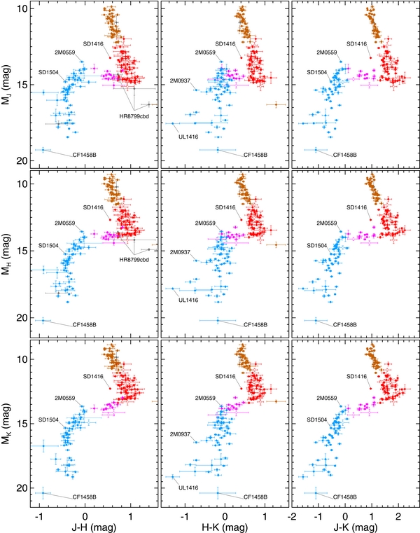
Figure 16. Color–magnitude diagrams in the MKO system showing all ultracool dwarfs from Table 10 with errors ⩽0.5 mag. Nearly half (40%) of the data points here use our new CFHT parallaxes. Symbol colors indicate spectral types: M6–L2 (brown), L2.5–L9 (red), L9.5–T4 (purple), ⩾T4.5 (blue), and unknown (gray). Solid symbols indicate photometry that is measured either directly or converted, e.g., from 2MASS to MKO, using the object's own spectrum. Open symbols indicate binary components where the flux ratio in one or more, but not all, bands was estimated from spectral decomposition. For one binary (SDSS J0805+4812), no symbol (i.e., error bar only) indicates that all flux ratios were estimated from spectral decomposition.
Download figure:
Standard image High-resolution image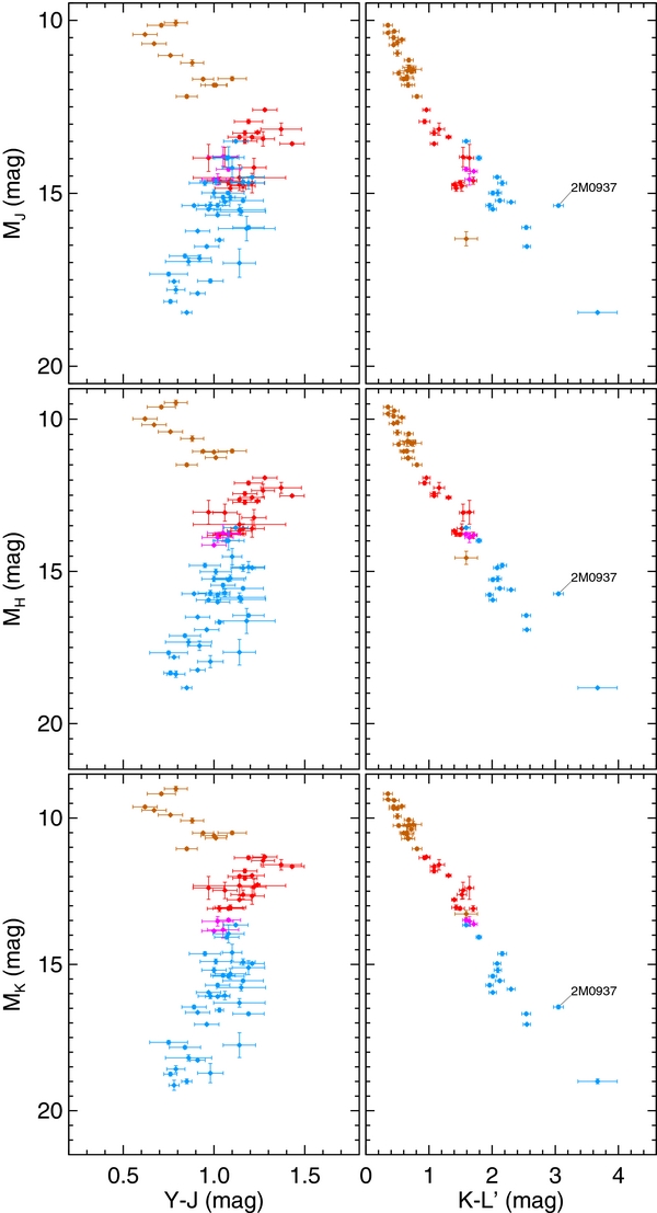
Figure 17. Same as Figure 16 but with Y − J and K − L' colors.
Download figure:
Standard image High-resolution image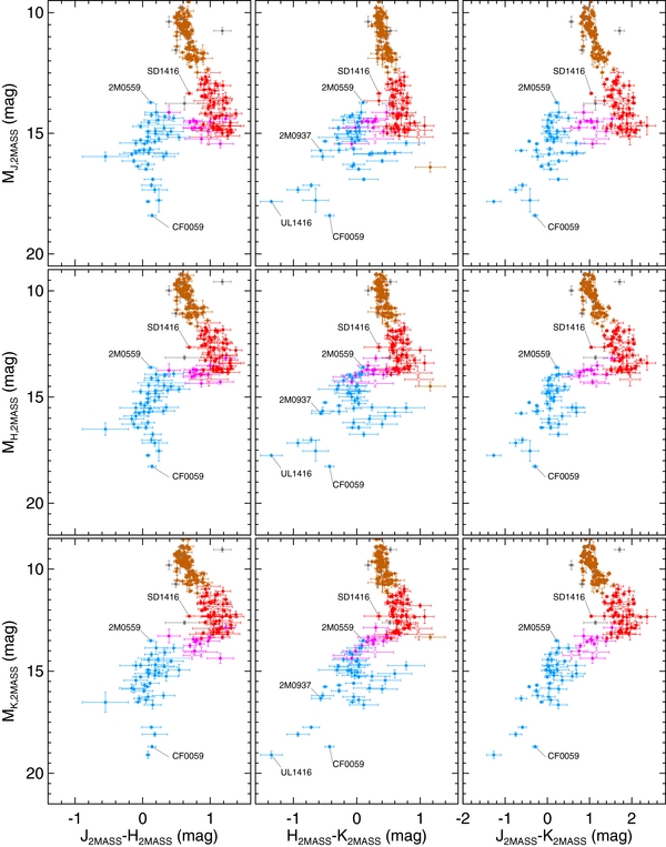
Figure 18. Same as Figure 16 but with photometry in the 2MASS system.
Download figure:
Standard image High-resolution image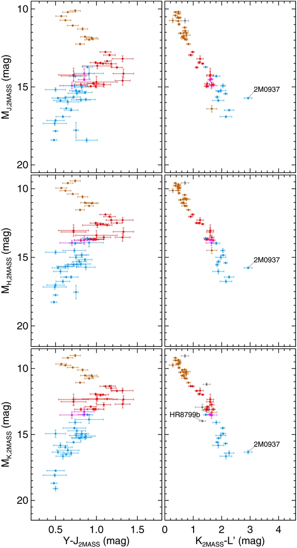
Figure 19. Same as Figure 17 but with JHK photometry in the 2MASS system.
Download figure:
Standard image High-resolution image
Download figure:
Standard image High-resolution image
Download figure:
Standard image High-resolution image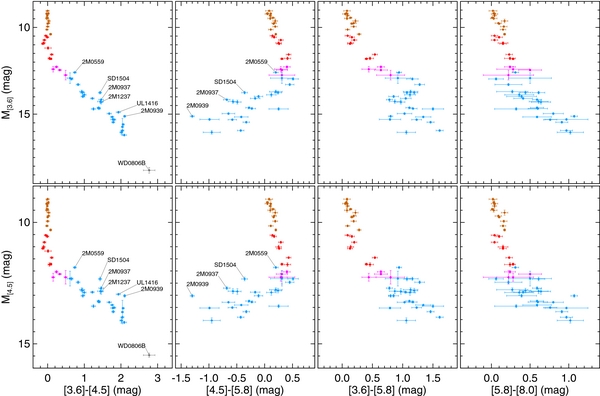
Figure 22. Color–magnitude diagrams of Spitzer/IRAC photometry showing all ultracool dwarfs from Table 11 with errors ⩽0.5 mag. Symbols are the same as in Figure 16.
Download figure:
Standard image High-resolution image
Figure 23. Same as Figure 22 but for the Spitzer/IRAC [5.8]- and [8.0]-band absolute magnitudes.
Download figure:
Standard image High-resolution image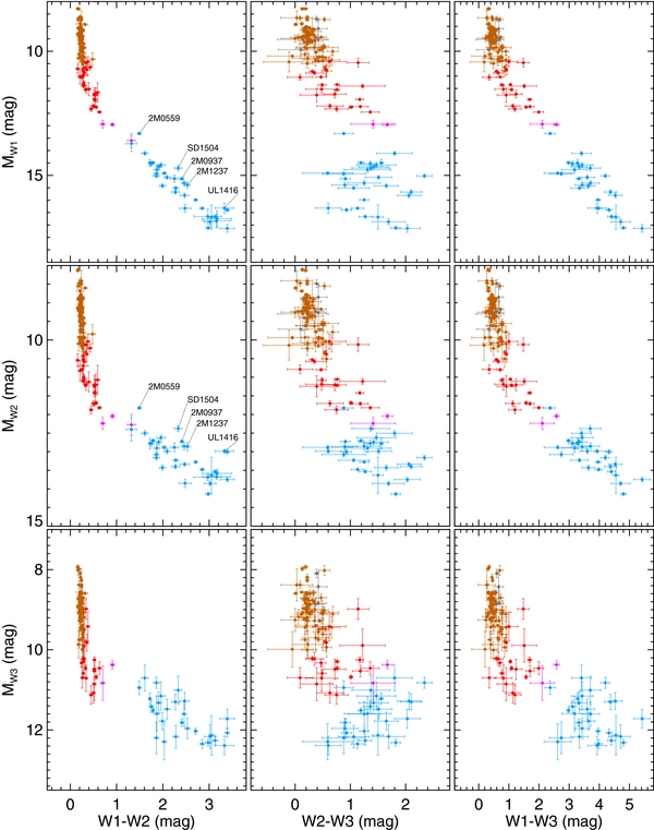
Figure 24. Color–magnitude diagrams of WISE photometry showing all ultracool dwarfs from Table 11 with errors ⩽0.5 mag. Symbols are the same as in Figure 16.
Download figure:
Standard image High-resolution imageFigures 25 and 26 show near-IR absolute magnitude as a function of spectral type, and Figures 27 and 28 show the same for the mid-IR. For these relations we have excluded subdwarfs, likely unresolved binaries (2MASS J0559−1404 and SDSS J1504+1027, see Section 6.2), and very low gravity objects. The last cut excludes planetary-mass objects (HR 8799bcde, 2M 1207b, and β Pic b) as well as very young objects in stellar associations: 2MASS J1207−3932 (TWA), PZ Tel B (β Pic), HR 7329B (β Pic), AB Pic b (Tuc-Hor), SSSPM J1102−3431 (TWA), and 2MASS J2234+4041AB (LkHα 233). We fit polynomials to the remaining field dwarf data, accounting for errors in both spectral types and absolute magnitudes in a Monte Carlo fashion. This is necessary as least-squares regression algorithms are unable to properly handle data sets in which the independent variables have errors, as in the case of our
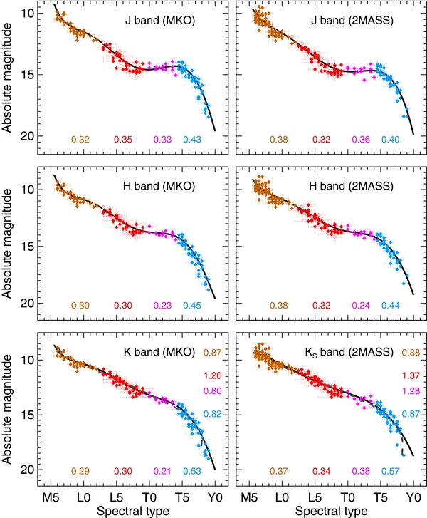
Figure 25. Near-IR absolute magnitude as a function of spectral type for all ultracool field dwarfs with parallaxes (photometry and spectral types from Table 10; subdwarfs and known young or planetary-mass objects excluded from plot). Thick solid lines are polynomial fits to the data (coefficients given in Table 14). At the bottom of each panel the rms about the fit is given, broken down by spectral type range: M6–L2 (brown), L2.5–L9 (red), L9.5–T4 (purple), and ⩾T4.5 (blue). Dashed gray lines show inverted polynomial fits, i.e., spectral type as a function of magnitude, for bands that are sufficiently monotonic (K and KS here). The rms about these fits for the same spectral type ranges as listed above are given along the right side of the respective panels. We use optical spectral types for M and L dwarfs when available (infrared types otherwise) and infrared types for T dwarfs.
Download figure:
Standard image High-resolution image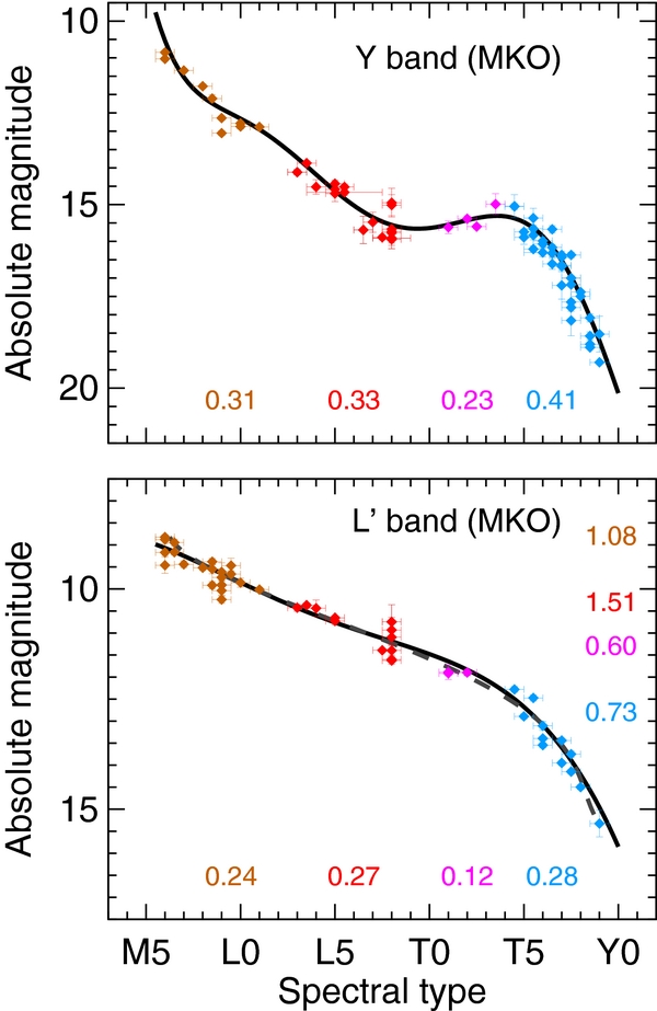
Figure 26. Same as Figure 25 but for Y- and L'-band absolute magnitudes.
Download figure:
Standard image High-resolution image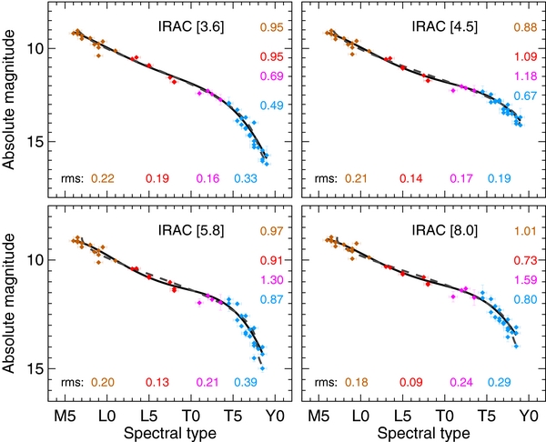
Download figure:
Standard image High-resolution image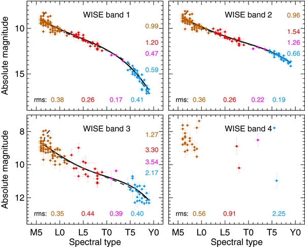
Download figure:
Standard image High-resolution imagespectral types. We drew 104 realizations of each data point with normally distributed magnitude errors and uniformly distributed spectral type errors. We then found the single best-fit polynomial to all N × 104 simulated points, using a standard least-squares method since all points now have equal weight. We fit magnitude as a function of spectral type for all bands, and for bands that were sufficiently monotonic in their decline we were able to also fit spectral type as a function of magnitude. The latter fits are applicable in the situation where an observer wishes to estimate the spectral type of an object based on photometry, whereas the more often quoted former fits are useful for spectroscopic distance estimates.
The coefficients of all of our polynomial fits are given in Table 14 along with the bulk rms of each fit. In Figures 25–28 the rms of the fits over specific spectral type ranges are also given. These rms values are useful in diagnosing the intrinsic scatter in absolute magnitude over different ranges of spectral types. They are also the relevant numbers to use, e.g., when determining a spectroscopic distance to a single object of known spectral type since T dwarfs generally show more scatter in absolute magnitude than L dwarfs, as opposed to adopting the single rms value given in Table 14. To test the impact of our choice of using optical types for M and L dwarfs when available, we tried using only infrared types for all objects. The median absolute value of the difference between polynomial fits computed these two ways was 0.01–0.02 mag for the MKO photometry and 0.03–0.06 mag for the 2MASS photometry. This is negligible compared to the scatter in the data about the fits, which is typically ≈0.4 mag, and thus using optical versus infrared spectral types does not significantly affect our results.
Table 14. Coefficients of Polynomial Fits to Absolute Magnitudes
| y | x | c0 | c1 | c2 | c3 | c4 | c5 | c6 | rms |
|---|---|---|---|---|---|---|---|---|---|
| YMKO | SpT | −3.51560 × 101 | 1.95444 × 101 | −3.26895 | 2.79438 × 10⁻¹ | −1.26151 × 10⁻² | 2.85027 × 10⁻⁴ | −2.52638 × 10⁻⁶ | 0.40 |
| JMKO | SpT | −2.83129 × 101 | 1.63986 × 101 | −2.74405 | 2.32771 × 10⁻¹ | −1.03332 × 10⁻² | 2.27641 × 10⁻⁴ | −1.94920 × 10⁻⁶ | 0.39 |
| HMKO | SpT | −2.97306 × 101 | 1.69138 × 101 | −2.85705 | 2.45209 × 10⁻¹ | −1.10960 × 10⁻² | 2.51601 × 10⁻⁴ | −2.24083 × 10⁻⁶ | 0.38 |
| KMKO | SpT | −1.52200 × 101 | 1.01248 × 101 | −1.63930 | 1.35177 × 10⁻¹ | −5.84342 × 10⁻³ | 1.25731 × 10⁻⁴ | −1.04935 × 10⁻⁶ | 0.40 |
| L'MKO | SpT | 8.89928 | −1.96584 × 10⁻¹ | 5.30581 × 10⁻² | −2.93191 × 10⁻³ | 5.46366 × 10⁻⁵ | 0.00000 | 0.00000 | 0.28 |
| J2MASS | SpT | −9.67994 | 8.16362 | −1.33053 | 1.11715 × 10⁻¹ | −4.82973 × 10⁻³ | 1.00820 × 10⁻⁴ | −7.84614 × 10⁻⁷ | 0.40 |
| H2MASS | SpT | −1.17526 × 101 | 9.00279 | −1.50370 | 1.29202 × 10⁻¹ | −5.80847 × 10⁻³ | 1.29363 × 10⁻⁴ | −1.11499 × 10⁻⁶ | 0.40 |
| K2MASS | SpT | 1.10114 × 101 | −8.67471 × 10⁻¹ | 1.34163 × 10⁻¹ | −6.42118 × 10⁻³ | 1.06693 × 10⁻⁴ | 0.00000 | 0.00000 | 0.43 |
| [3.6] | SpT | 9.34220 | −3.35222 × 10⁻¹ | 6.91081 × 10⁻² | −3.60108 × 10⁻³ | 6.50191 × 10⁻⁵ | ... | ... | 0.29 |
| [4.5] | SpT | 9.73946 | −4.39968 × 10⁻¹ | 7.65343 × 10⁻² | −3.63435 × 10⁻³ | 5.82107 × 10⁻⁵ | ... | ... | 0.22 |
| [5.8] | SpT | 1.10834 × 101 | −9.01820 × 10⁻¹ | 1.29019 × 10⁻¹ | −6.22795 × 10⁻³ | 1.03507 × 10⁻⁴ | ... | ... | 0.32 |
| [8.0] | SpT | 9.97853 | −5.29595 × 10⁻¹ | 8.43465 × 10⁻² | −4.12294 × 10⁻³ | 6.89733 × 10⁻⁵ | ... | ... | 0.27 |
| W1 | SpT | 7.14765 | 3.55395 × 10⁻¹ | −4.38105 × 10⁻³ | −3.33944 × 10⁻⁴ | 1.58040 × 10⁻⁵ | ... | ... | 0.39 |
| W2 | SpT | 7.46564 | 1.92354 × 10⁻¹ | 1.14325 × 10⁻² | −8.81973 × 10⁻⁴ | 1.78555 × 10⁻⁵ | ... | ... | 0.35 |
| W3 | SpT | 7.81181 | 6.64242 × 10⁻² | 2.01740 × 10⁻² | −1.28563 × 10⁻³ | 2.37656 × 10⁻⁵ | ... | ... | 0.43 |
| W4 | SpT | 7.78974 | 1.14630 × 10⁻¹ | −2.16042 × 10⁻³ | ... | ... | ... | ... | 0.76 |
| SpT | KMKO | 2.61198 × 10³ | −1.20348 × 10³ | 2.28908 × 10² | −2.30427 × 101 | 1.29813 | −3.87650 × 10⁻² | 4.78483 × 10⁻⁴ | 1.08 |
| SpT | K2MASS | 3.16377 × 10² | −9.80581 × 101 | 1.09318 × 101 | −5.04080 × 10⁻¹ | 8.33390 × 10⁻³ | 0.00000 | 0.00000 | 1.20 |
| SpT | L'MKO | 9.42393 × 10² | −3.26016 × 10² | 4.10902 × 101 | −2.21930 | 4.38768 × 10⁻² | 0.00000 | 0.00000 | 1.26 |
| SpT | [3.6] | 7.37848 × 10² | −2.50242 × 10² | 3.08566 × 101 | −1.62281 | 3.11677 × 10⁻² | ... | ... | 0.79 |
| SpT | [4.5] | 3.46964 × 10² | −9.45512 × 101 | 7.99261 | −1.57271 × 10⁻¹ | −3.36767 × 10⁻³ | ... | ... | 0.98 |
| SpT | [5.8] | 1.87732 × 10³ | −6.47450 × 10² | 8.19571 × 101 | −4.49580 | 9.07889 × 10⁻² | ... | ... | 1.08 |
| SpT | [8.0] | 2.79433 × 10³ | −9.82793 × 10² | 1.27367 × 10² | −7.19295 | 1.50118 × 10⁻¹ | ... | ... | 1.14 |
| SpT | W1 | 5.54038 × 10² | −1.83014 × 10² | 2.19510 × 101 | −1.11687 | 2.07063 × 10⁻² | ... | ... | 1.18 |
| SpT | W2 | 3.65904 × 10² | −1.07813 × 10² | 1.06860 × 101 | −3.71750 × 10⁻¹ | 2.55541 × 10⁻³ | ... | ... | 1.29 |
| SpT | W3 | −1.39856 × 10² | 1.37418 × 10² | −3.28946 × 101 | 2.98984 | −9.21404 × 10⁻² | ... | ... | 2.42 |
Notes. These polynomial fits are applicable from spectral types of M6 to T9 (inclusive), with the exceptions of H2MASS, K2MASS, [5.8], and [8.0] (M6–T8.5). The coefficients are defined as y = ∑i = 0cixi, where y and x are the quantities listed in the first two columns. Numerical spectral types are defined such that M6 = 6 and T9 = 29. We use optical spectral types for M and L dwarfs when available, infrared types otherwise, and infrared types for T dwarfs. (As described in the text, using infrared types for all objects would result in polynomial relations different by 0.01–0.02 mag for MKO bands and 0.03–0.06 mag for 2MASS bands, i.e., negligible compared to the scatter about the fits.) The rightmost column gives the rms about the fit over all spectral types. Note that the rms may be significantly different over more restricted ranges of spectral type as discussed in Section 5.3 and shown in Figures 25–28.
Download table as: ASCIITypeset image
We have also tabulated the mean absolute magnitude at each spectral type in Tables 15–18, and we plot the resulting values in Figures 29 and 30. This information enables a more direct way of assessing the changes in broadband fluxes as a function of spectral type, since polynomial fits are not guaranteed to be a good description of the data. In these tables we give the weighted average along with the rms for "normal" field dwarfs (i.e., those not flagged as atypical in Table 9). We also quantify the level of intrinsic scatter at each spectral type by computing χ2 for each type's collection of measurements and finding the amount of additional magnitude error that is needed to make reduced χ2 ≈ 1, i.e., p(χ2) = 0.5. When there are small numbers of objects in a bin, or when the measurement errors are large, the additional error needed is typically small, but this does not necessarily mean that the intrinsic scatter is small. Thus, the value we find for the needed additional error is only a lower limit to the intrinsic scatter at a given spectral type.
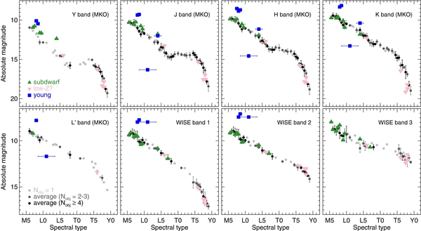
Figure 29. Gray and black circles show the weighted averages of absolute magnitudes for normal field dwarfs as a function of spectral type with error bars showing the rms among objects of a given type (Tables 15–18). We also show individual objects that were not considered to be normal field dwarfs: known subdwarfs as determined from optical spectroscopy (green triangles), suspected low-metallicity brown dwarfs (pink upside-down triangles), and members of young moving groups, including planetary-mass companions (blue squares; the underluminous young object is 2M 1207b). The objects plotted here are marked in the "Note" column in Table 9 and are excluded from our analysis of absolute magnitudes as a function of spectral type, along with overluminous objects suspected to be unresolved binaries (not shown here).
Download figure:
Standard image High-resolution image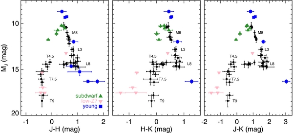
Figure 30. Color–magnitude diagrams on the MKO system, where black circles show weighted averages of normal field dwarf magnitudes in spectral type bins from M6 to T9 (see Table 15; only bins with two or more objects are shown). Error bars indicate the rms in absolute magnitude and color for each bin. Individual objects that were not considered to be normal field dwarfs are also shown: known subdwarfs as determined from optical spectroscopy (green triangles), suspected low-metallicity brown dwarfs (pink upside-down triangles), and members of young moving groups, including planetary-mass companions (blue squares).
Download figure:
Standard image High-resolution imageTable 15. Mean MKO Absolute Magnitudes as a Function of Spectral Type
| Spectral | Y Band | J Band | H Band | K Band | L' Band | |||||||||||||||
|---|---|---|---|---|---|---|---|---|---|---|---|---|---|---|---|---|---|---|---|---|
| Type | Mean | rms | σadd | N | Mean | rms | σadd | N | Mean | rms | σadd | N | Mean | rms | σadd | N | Mean | rms | σadd | N |
| M6 | 10.94 ± 0.04 | 0.13 | ... | 2 | 10.34 ± 0.02 | 0.27 | 0.12 | 5 | 9.82 ± 0.03 | 0.28 | 0.13 | 5 | 9.40 ± 0.03 | 0.34 | 0.16 | 5 | 8.95 ± 0.04 | 0.29 | 0.07 | 4 |
| M6.5 | ... | ... | ... | 0 | 10.45 ± 0.03 | 0.16 | 0.03 | 3 | 9.89 ± 0.03 | 0.20 | 0.06 | 3 | 9.52 ± 0.03 | 0.15 | 0.01 | 3 | 9.08 ± 0.05 | 0.15 | ... | 2 |
| M7 | 11.34 ± 0.06 | ... | ... | 1 | 10.31 ± 0.02 | 0.42 | 0.33 | 5 | 9.94 ± 0.02 | 0.40 | 0.31 | 5 | 9.50 ± 0.02 | 0.36 | 0.29 | 5 | 9.44 ± 0.08 | ... | ... | 1 |
| M7.5 | ... | ... | ... | 0 | 10.82 ± 0.05 | ... | ... | 1 | 10.26 ± 0.05 | ... | ... | 1 | 9.79 ± 0.05 | ... | ... | 1 | ... | ... | ... | 0 |
| M8 | 11.77 ± 0.06 | ... | ... | 1 | 10.99 ± 0.02 | 0.26 | 0.12 | 6 | 10.40 ± 0.02 | 0.23 | 0.11 | 6 | 9.88 ± 0.02 | 0.26 | ... | 5 | 9.52 ± 0.07 | ... | ... | 1 |
| M8.5 | 12.11 ± 0.11 | ... | ... | 1 | 11.40 ± 0.03 | 0.19 | 0.13 | 5 | 10.77 ± 0.03 | 0.21 | 0.15 | 5 | 10.28 ± 0.03 | 0.20 | 0.14 | 5 | 9.61 ± 0.05 | 0.27 | 0.12 | 3 |
| M9 | 12.82 ± 0.04 | 0.29 | 0.10 | 2 | 11.80 ± 0.03 | 0.30 | 0.22 | 5 | 11.15 ± 0.03 | 0.32 | 0.24 | 5 | 10.62 ± 0.02 | 0.33 | 0.25 | 5 | 9.93 ± 0.03 | 0.25 | 0.15 | 5 |
| M9.5 | ... | ... | ... | 0 | 11.50 ± 0.05 | 0.19 | 0.01 | 3 | 10.84 ± 0.05 | 0.21 | 0.06 | 3 | 10.40 ± 0.04 | 0.16 | 0.05 | 3 | 9.63 ± 0.07 | 0.14 | ... | 2 |
| L0 | 12.83 ± 0.05 | 0.06 | ... | 2 | 11.69 ± 0.02 | 0.18 | 0.14 | 5 | 11.04 ± 0.02 | 0.14 | 0.09 | 5 | 10.46 ± 0.03 | 0.15 | 0.09 | 4 | 9.86 ± 0.10 | ... | ... | 1 |
| L0.5 | ... | ... | ... | 0 | ... | ... | ... | 0 | ... | ... | ... | 0 | ... | ... | ... | 0 | ... | ... | ... | 0 |
| L1 | 12.88 ± 0.05 | ... | ... | 1 | 11.87 ± 0.03 | ... | ... | 1 | 11.26 ± 0.03 | 0.09 | ... | 2 | 10.66 ± 0.03 | 0.11 | 0.03 | 2 | 10.01 ± 0.05 | ... | ... | 1 |
| L1.5 | ... | ... | ... | 0 | 12.20 ± 0.04 | 0.27 | 0.27 | 2 | 11.51 ± 0.04 | 0.21 | 0.18 | 2 | 10.69 ± 0.11 | ... | ... | 1 | ... | ... | ... | 0 |
| L2 | ... | ... | ... | 0 | 12.18 ± 0.12 | ... | ... | 1 | 11.45 ± 0.12 | ... | ... | 1 | 10.82 ± 0.12 | ... | ... | 1 | ... | ... | ... | 0 |
| L2.5 | ... | ... | ... | 0 | ... | ... | ... | 0 | ... | ... | ... | 0 | ... | ... | ... | 0 | ... | ... | ... | 0 |
| L3 | 14.12 ± 0.07 | ... | ... | 1 | 12.81 ± 0.03 | 0.27 | 0.22 | 3 | 11.97 ± 0.03 | 0.28 | 0.25 | 3 | 11.26 ± 0.03 | 0.29 | 0.27 | 3 | 10.43 ± 0.08 | ... | ... | 1 |
| L3.5 | 13.87 ± 0.06 | ... | ... | 1 | 12.59 ± 0.03 | ... | ... | 1 | 11.93 ± 0.03 | ... | ... | 1 | 11.33 ± 0.03 | ... | ... | 1 | 10.37 ± 0.05 | ... | ... | 1 |
| L4 | 14.52 ± 0.20 | ... | ... | 1 | 12.83 ± 0.04 | 0.24 | 0.15 | 5 | 12.14 ± 0.05 | 0.24 | 0.13 | 5 | 11.25 ± 0.03 | 0.29 | 0.22 | 5 | 10.44 ± 0.19 | ... | ... | 1 |
| L4.5 | ... | ... | ... | 0 | 13.74 ± 0.05 | 0.24 | 0.28 | 3 | 12.68 ± 0.04 | 0.20 | 0.22 | 3 | 11.76 ± 0.03 | 0.28 | 0.39 | 3 | ... | ... | ... | 0 |
| L5 | 14.54 ± 0.05 | 0.14 | ... | 3 | 13.44 ± 0.03 | 0.48 | 0.46 | 6 | 12.61 ± 0.03 | 0.39 | 0.37 | 6 | 11.96 ± 0.02 | 0.34 | 0.35 | 6 | 10.66 ± 0.03 | 0.05 | ... | 2 |
| L5.5 | 14.58 ± 0.06 | 0.10 | ... | 2 | 13.49 ± 0.04 | 0.27 | 0.26 | 5 | 12.71 ± 0.04 | 0.28 | 0.29 | 5 | 11.99 ± 0.03 | 0.24 | 0.25 | 5 | ... | ... | ... | 0 |
| L6 | ... | ... | ... | 0 | 14.12 ± 0.09 | 0.48 | 0.57 | 3 | 13.05 ± 0.06 | 0.37 | 0.43 | 3 | 12.00 ± 0.03 | 0.35 | 0.51 | 3 | ... | ... | ... | 0 |
| L6.5 | 15.69 ± 0.37 | ... | ... | 1 | 14.21 ± 0.03 | 0.23 | 0.15 | 4 | 13.29 ± 0.02 | 0.18 | 0.17 | 4 | 12.56 ± 0.03 | 0.24 | 0.30 | 4 | ... | ... | ... | 0 |
| L7 | 15.48 ± 0.27 | ... | ... | 1 | 14.67 ± 0.08 | 0.29 | 0.26 | 3 | 13.70 ± 0.07 | 0.34 | 0.34 | 3 | 12.89 ± 0.06 | 0.35 | 0.38 | 3 | ... | ... | ... | 0 |
| L7.5 | 15.89 ± 0.06 | ... | ... | 1 | 14.74 ± 0.03 | 0.20 | ... | 3 | 13.73 ± 0.03 | 0.16 | 0.21 | 3 | 12.91 ± 0.03 | 0.42 | 0.41 | 2 | 11.39 ± 0.04 | ... | ... | 1 |
| L8 | 15.76 ± 0.04 | 0.41 | 0.28 | 8 | 14.68 ± 0.03 | 0.39 | 0.28 | 9 | 13.77 ± 0.03 | 0.36 | 0.27 | 9 | 13.05 ± 0.03 | 0.33 | 0.28 | 9 | 11.52 ± 0.04 | 0.36 | 0.26 | 6 |
| L8.5 | ... | ... | ... | 0 | 14.59 ± 0.04 | 0.18 | 0.20 | 4 | 13.76 ± 0.04 | 0.06 | ... | 4 | 13.04 ± 0.04 | 0.11 | 0.10 | 4 | ... | ... | ... | 0 |
| L9 | ... | ... | ... | 0 | 14.33 ± 0.07 | 0.34 | 0.27 | 2 | 13.48 ± 0.06 | 0.24 | 0.19 | 2 | 12.73 ± 0.07 | 0.25 | 0.19 | 2 | ... | ... | ... | 0 |
| L9.5 | ... | ... | ... | 0 | ... | ... | ... | 0 | ... | ... | ... | 0 | ... | ... | ... | 0 | ... | ... | ... | 0 |
| T0 | ... | ... | ... | 0 | 14.24 ± 0.07 | 0.27 | 0.39 | 2 | 13.52 ± 0.07 | 0.41 | 0.59 | 2 | 13.17 ± 0.07 | 0.26 | 0.38 | 2 | ... | ... | ... | 0 |
| T0.5 | ... | ... | ... | 0 | ... | ... | ... | 0 | ... | ... | ... | 0 | ... | ... | ... | 0 | ... | ... | ... | 0 |
| T1 | 15.62 ± 0.17 | ... | ... | 1 | 14.37 ± 0.02 | 0.16 | 0.30 | 2 | 13.81 ± 0.02 | 0.06 | ... | 2 | 13.62 ± 0.02 | 0.07 | ... | 2 | 11.91 ± 0.05 | 0.02 | ... | 2 |
| T1.5 | ... | ... | ... | 0 | 14.44 ± 0.06 | ... | ... | 1 | 14.03 ± 0.07 | ... | ... | 1 | 13.91 ± 0.09 | ... | ... | 1 | ... | ... | ... | 0 |
| T2 | 15.39 ± 0.08 | ... | ... | 1 | 14.43 ± 0.04 | 0.19 | 0.27 | 2 | 13.88 ± 0.04 | 0.14 | 0.20 | 2 | 13.58 ± 0.05 | 0.19 | 0.28 | 2 | 11.90 ± 0.07 | ... | ... | 1 |
| T2.5 | 15.60 ± 0.06 | ... | ... | 1 | 14.50 ± 0.03 | 0.34 | 0.58 | 2 | 14.01 ± 0.03 | 0.36 | 0.60 | 2 | 13.78 ± 0.03 | 0.23 | 0.38 | 2 | ... | ... | ... | 0 |
| T3 | ... | ... | ... | 0 | ... | ... | ... | 0 | ... | ... | ... | 0 | ... | ... | ... | 0 | ... | ... | ... | 0 |
| T3.5 | 14.99 ± 0.29 | ... | ... | 1 | 14.44 ± 0.06 | 0.35 | 0.38 | 3 | 13.97 ± 0.07 | 0.19 | 0.14 | 3 | 13.90 ± 0.08 | 0.29 | 0.31 | 3 | ... | ... | ... | 0 |
| T4 | ... | ... | ... | 0 | 15.04 ± 0.18 | ... | ... | 1 | 14.41 ± 0.16 | ... | ... | 1 | 14.13 ± 0.26 | ... | ... | 1 | ... | ... | ... | 0 |
| T4.5 | 15.05 ± 0.08 | 0.00 | ... | 2 | 14.21 ± 0.04 | 0.28 | 0.29 | 4 | 14.28 ± 0.04 | 0.34 | 0.35 | 4 | 14.42 ± 0.04 | 0.43 | 0.45 | 4 | 12.28 ± 0.07 | ... | ... | 1 |
| T5 | 15.76 ± 0.06 | 0.10 | ... | 2 | 14.43 ± 0.03 | 0.32 | 0.32 | 7 | 14.66 ± 0.03 | 0.35 | 0.38 | 7 | 14.81 ± 0.03 | 0.39 | 0.41 | 7 | 12.89 ± 0.06 | ... | ... | 1 |
| T5.5 | 15.90 ± 0.05 | 0.35 | 0.25 | 4 | 14.72 ± 0.04 | 0.32 | 0.34 | 6 | 14.83 ± 0.04 | 0.26 | 0.25 | 6 | 14.77 ± 0.04 | 0.29 | 0.26 | 6 | 12.47 ± 0.07 | ... | ... | 1 |
| T6 | 16.04 ± 0.06 | 0.06 | ... | 2 | 15.22 ± 0.02 | 0.15 | 0.16 | 3 | 15.56 ± 0.02 | 0.20 | 0.22 | 3 | 15.77 ± 0.02 | 0.33 | 0.37 | 3 | 13.41 ± 0.04 | 0.22 | 0.16 | 3 |
| T6.5 | 16.13 ± 0.05 | 0.39 | 0.31 | 4 | 15.22 ± 0.03 | 0.31 | 0.32 | 6 | 15.60 ± 0.03 | 0.47 | 0.46 | 6 | 15.71 ± 0.03 | 0.66 | 0.67 | 6 | ... | ... | ... | 0 |
| T7 | 16.57 ± 0.04 | 0.33 | 0.27 | 4 | 15.54 ± 0.03 | 0.25 | 0.13 | 4 | 15.97 ± 0.03 | 0.34 | 0.16 | 4 | 16.01 ± 0.03 | 0.15 | 0.12 | 3 | 13.95 ± 0.06 | ... | ... | 1 |
| T7.5 | 17.15 ± 0.03 | 0.64 | 0.61 | 6 | 16.05 ± 0.02 | 0.65 | 0.70 | 7 | 16.42 ± 0.02 | 0.70 | 0.77 | 7 | 16.62 ± 0.02 | 0.83 | 0.80 | 6 | 14.02 ± 0.04 | 0.28 | 0.11 | 2 |
| T8 | 17.42 ± 0.04 | 0.08 | 0.05 | 2 | 16.39 ± 0.03 | 0.35 | 0.46 | 3 | 16.77 ± 0.03 | 0.32 | 0.43 | 3 | 16.88 ± 0.03 | 0.31 | 0.46 | 3 | 14.50 ± 0.05 | ... | ... | 1 |
| T8.5 | 18.76 ± 0.03 | 0.36 | 0.45 | 4 | 17.81 ± 0.03 | 0.33 | 0.37 | 4 | 18.14 ± 0.03 | 0.33 | 0.36 | 4 | 18.26 ± 0.03 | 0.48 | 0.54 | 4 | ... | ... | ... | 0 |
| T9 | 19.29 ± 0.03 | 0.54 | 0.43 | 2 | 18.42 ± 0.03 | 0.66 | 0.75 | 2 | 18.81 ± 0.03 | 0.66 | 0.74 | 2 | 18.97 ± 0.08 | 0.54 | 0.48 | 2 | 15.33 ± 0.30 | ... | ... | 1 |
Notes. For each band the weighted average and standard error are given ("mean" column) as computed from all objects of a given spectral type with measured photometry (see Table 12). The rms of those objects is also given, which includes the scatter due to both measurement errors and intrinsic variations at that spectral type. The σadd column additional uncertainty needed to make p(χ2) = 0.5 (i.e., reduced χ2 ≈ 1) for the set of magnitudes. This is essentially a lower limit on the intrinsic scatter because scatter due to measurement error can always mask intrinsic variations at some level and because small sample sizes at some spectral types may not fully capture the intrinsic variations. The N column notes how many objects were used to derive the mean, rms, and σadd; when N = 1 the "mean" is simply the magnitude of the one object available. We only use "normal" field dwarfs, i.e., those not flagged as atypical in Table 9, to compute the weighted averages. When individual object magnitude errors are large enough to explain the observed scatter (i.e., p(χ2) > 0.5) no value for σadd is listed. Note that we use optical spectral types for M and L dwarfs when available (infrared types otherwise) and infrared types for T dwarfs.
Table 16. Mean 2MASS Absolute Magnitudes as a Function of Spectral Type
| Spectral | J Band | H Band | KS Band | |||||||||
|---|---|---|---|---|---|---|---|---|---|---|---|---|
| Type | Mean | rms | σadd | N | Mean | rms | σadd | N | Mean | rms | σadd | N |
| M6 | 10.28 ± 0.01 | 0.27 | 0.25 | 16 | 9.73 ± 0.01 | 0.27 | 0.26 | 16 | 9.31 ± 0.01 | 0.28 | 0.28 | 16 |
| M6.5 | 10.33 ± 0.01 | 0.44 | 0.44 | 16 | 9.75 ± 0.01 | 0.45 | 0.44 | 16 | 9.41 ± 0.01 | 0.44 | 0.43 | 16 |
| M7 | 10.25 ± 0.02 | 0.45 | 0.48 | 8 | 9.79 ± 0.02 | 0.45 | 0.47 | 8 | 9.42 ± 0.01 | 0.44 | 0.46 | 8 |
| M7.5 | 10.63 ± 0.02 | 0.30 | 0.31 | 9 | 10.01 ± 0.02 | 0.32 | 0.33 | 9 | 9.61 ± 0.02 | 0.33 | 0.34 | 9 |
| M8 | 10.93 ± 0.01 | 0.46 | 0.34 | 11 | 10.24 ± 0.01 | 0.46 | 0.34 | 11 | 9.83 ± 0.01 | 0.44 | 0.35 | 12 |
| M8.5 | 11.58 ± 0.01 | 0.20 | 0.20 | 9 | 10.88 ± 0.01 | 0.23 | 0.23 | 9 | 10.46 ± 0.01 | 0.22 | 0.23 | 9 |
| M9 | 11.81 ± 0.02 | 0.29 | 0.26 | 7 | 11.10 ± 0.02 | 0.31 | 0.29 | 7 | 10.57 ± 0.02 | 0.30 | 0.30 | 8 |
| M9.5 | 11.69 ± 0.03 | 0.14 | 0.12 | 6 | 10.89 ± 0.03 | 0.20 | 0.20 | 6 | 10.37 ± 0.03 | 0.22 | 0.23 | 6 |
| L0 | 11.77 ± 0.03 | 0.21 | 0.17 | 6 | 10.99 ± 0.02 | 0.18 | 0.11 | 6 | 10.53 ± 0.02 | 0.15 | 0.12 | 7 |
| L0.5 | ... | ... | ... | 0 | ... | ... | ... | 0 | ... | ... | ... | 0 |
| L1 | 11.96 ± 0.02 | 0.01 | ... | 3 | 11.22 ± 0.02 | 0.07 | 0.06 | 4 | 10.69 ± 0.02 | 0.11 | 0.12 | 4 |
| L1.5 | 12.07 ± 0.12 | 0.41 | 0.31 | 2 | 11.32 ± 0.11 | 0.32 | 0.22 | 2 | 10.94 ± 0.04 | 0.23 | 0.22 | 3 |
| L2 | 12.36 ± 0.11 | ... | ... | 1 | 11.40 ± 0.11 | ... | ... | 1 | 10.79 ± 0.11 | ... | ... | 1 |
| L2.5 | 12.66 ± 0.20 | ... | ... | 1 | 11.73 ± 0.20 | ... | ... | 1 | 10.98 ± 0.20 | ... | ... | 1 |
| L3 | 12.87 ± 0.03 | 0.20 | 0.19 | 4 | 11.92 ± 0.02 | 0.22 | 0.25 | 4 | 11.27 ± 0.03 | 0.22 | 0.26 | 4 |
| L3.5 | 12.77 ± 0.03 | 0.13 | 0.22 | 2 | 11.88 ± 0.03 | 0.01 | ... | 2 | 11.35 ± 0.02 | 0.04 | ... | 2 |
| L4 | 13.09 ± 0.05 | 0.20 | ... | 6 | 12.11 ± 0.05 | 0.43 | 0.37 | 7 | 11.55 ± 0.04 | 0.28 | 0.23 | 7 |
| L4.5 | 13.81 ± 0.05 | 0.23 | 0.25 | 3 | 12.62 ± 0.04 | 0.20 | 0.23 | 3 | 11.79 ± 0.03 | 0.28 | 0.39 | 3 |
| L5 | 13.56 ± 0.03 | 0.44 | 0.46 | 7 | 12.59 ± 0.02 | 0.36 | 0.37 | 7 | 11.99 ± 0.02 | 0.31 | 0.35 | 7 |
| L5.5 | 13.58 ± 0.04 | 0.27 | 0.27 | 5 | 12.64 ± 0.04 | 0.28 | 0.29 | 5 | 12.01 ± 0.04 | 0.26 | 0.26 | 5 |
| L6 | 14.34 ± 0.09 | 0.47 | 0.57 | 3 | 12.98 ± 0.06 | 0.38 | 0.44 | 3 | 12.03 ± 0.03 | 0.34 | 0.52 | 3 |
| L6.5 | 14.33 ± 0.03 | 0.19 | 0.01 | 4 | 13.25 ± 0.03 | 0.16 | 0.11 | 4 | 12.55 ± 0.03 | 0.19 | 0.21 | 4 |
| L7 | 14.76 ± 0.08 | 0.40 | 0.45 | 3 | 13.64 ± 0.07 | 0.38 | 0.37 | 3 | 12.89 ± 0.06 | 0.33 | 0.37 | 3 |
| L7.5 | 14.93 ± 0.03 | 0.11 | 0.08 | 2 | 13.70 ± 0.03 | 0.20 | 0.19 | 2 | 13.01 ± 0.03 | 0.25 | 0.36 | 3 |
| L8 | 14.81 ± 0.04 | 0.30 | 0.09 | 9 | 13.70 ± 0.03 | 0.33 | 0.16 | 9 | 13.06 ± 0.03 | 0.30 | 0.20 | 9 |
| L8.5 | 14.77 ± 0.05 | 0.21 | 0.20 | 4 | 13.72 ± 0.05 | 0.08 | ... | 4 | 13.05 ± 0.04 | 0.16 | 0.15 | 4 |
| L9 | 14.63 ± 0.05 | 0.40 | 0.48 | 3 | 13.59 ± 0.05 | 0.28 | 0.32 | 3 | 12.95 ± 0.05 | 0.36 | 0.43 | 3 |
| L9.5 | ... | ... | ... | 0 | ... | ... | ... | 0 | ... | ... | ... | 0 |
| T0 | 14.45 ± 0.10 | 0.09 | ... | 2 | 13.29 ± 0.11 | 0.25 | 0.34 | 2 | 13.24 ± 0.09 | 0.33 | 0.54 | 2 |
| T0.5 | ... | ... | ... | 0 | ... | ... | ... | 0 | ... | ... | ... | 0 |
| T1 | 14.50 ± 0.02 | 0.30 | 0.59 | 2 | 13.72 ± 0.02 | 0.16 | 0.28 | 2 | 13.55 ± 0.02 | 0.02 | ... | 2 |
| T1.5 | 14.76 ± 0.13 | ... | ... | 1 | 13.99 ± 0.13 | ... | ... | 1 | 14.01 ± 0.17 | ... | ... | 1 |
| T2 | 14.68 ± 0.04 | 0.17 | 0.24 | 2 | 13.82 ± 0.04 | 0.13 | 0.18 | 2 | 13.56 ± 0.05 | 0.12 | 0.17 | 2 |
| T2.5 | 14.74 ± 0.09 | 0.69 | 1.10 | 2 | 14.00 ± 0.08 | 0.41 | 0.59 | 2 | 13.67 ± 0.13 | 0.66 | 1.06 | 2 |
| T3 | ... | ... | ... | 0 | ... | ... | ... | 0 | ... | ... | ... | 0 |
| T3.5 | 14.62 ± 0.06 | 0.33 | 0.35 | 3 | 13.91 ± 0.07 | 0.16 | 0.12 | 3 | 13.82 ± 0.09 | 0.47 | 0.50 | 3 |
| T4 | 15.23 ± 0.18 | ... | ... | 1 | 14.36 ± 0.16 | ... | ... | 1 | 14.07 ± 0.24 | ... | ... | 1 |
| T4.5 | 14.51 ± 0.04 | 0.28 | 0.26 | 4 | 14.23 ± 0.06 | 0.29 | 0.28 | 4 | 14.49 ± 0.06 | 0.39 | 0.45 | 4 |
| T5 | 14.81 ± 0.03 | 0.31 | 0.32 | 6 | 14.66 ± 0.03 | 0.38 | 0.41 | 6 | 14.69 ± 0.05 | 0.41 | 0.41 | 6 |
| T5.5 | 15.08 ± 0.04 | 0.32 | 0.31 | 5 | 14.80 ± 0.06 | 0.36 | 0.32 | 5 | 14.59 ± 0.05 | 0.32 | 0.30 | 5 |
| T6 | 15.35 ± 0.02 | 0.11 | 0.09 | 5 | 15.32 ± 0.02 | 0.17 | 0.19 | 5 | 15.68 ± 0.01 | 0.33 | 0.50 | 5 |
| T6.5 | 15.66 ± 0.04 | 0.32 | 0.31 | 6 | 15.48 ± 0.07 | 0.61 | 0.64 | 6 | 15.76 ± 0.07 | 0.71 | 0.73 | 6 |
| T7 | 15.85 ± 0.05 | 0.03 | ... | 3 | 15.72 ± 0.10 | 0.27 | 0.19 | 3 | 15.43 ± 0.12 | 0.38 | 0.29 | 3 |
| T7.5 | 16.37 ± 0.02 | 0.55 | 0.47 | 5 | 16.43 ± 0.03 | 0.53 | 0.45 | 5 | 16.59 ± 0.02 | 0.83 | 0.73 | 5 |
| T8 | 16.69 ± 0.05 | 0.44 | 0.38 | 2 | 16.47 ± 0.08 | 0.39 | 0.31 | 2 | 16.42 ± 0.13 | 0.28 | 0.15 | 2 |
| T8.5 | 18.41 ± 0.05 | ... | ... | 1 | 18.27 ± 0.07 | ... | ... | 1 | 18.70 ± 0.07 | ... | ... | 1 |
| T9 | 18.37 ± 0.13 | 0.45 | 0.16 | 2 | 17.54 ± 0.49 | ... | ... | 1 | 18.19 ± 0.53 | ... | ... | 1 |
Note. Same as Table 15 but for 2MASS magnitudes.
Download table as: ASCIITypeset image
Table 17. Mean Spitzer/IRAC Absolute Magnitudes as a Function of Spectral Type
| Spectral | [3.6] Band | [4.5] Band | [5.8] Band | [8.0] Band | ||||||||||||
|---|---|---|---|---|---|---|---|---|---|---|---|---|---|---|---|---|
| Type | Mean | rms | σadd | N | Mean | rms | σadd | N | Mean | rms | σadd | N | Mean | rms | σadd | N |
| M6 | 9.19 ± 0.01 | ... | ... | 1 | 9.17 ± 0.02 | ... | ... | 1 | 9.12 ± 0.01 | ... | ... | 1 | 9.09 ± 0.01 | ... | ... | 1 |
| M6.5 | 9.10 ± 0.03 | 0.10 | ... | 3 | 9.14 ± 0.03 | 0.11 | ... | 3 | 9.09 ± 0.03 | 0.11 | ... | 3 | 8.99 ± 0.02 | 0.10 | 0.00 | 3 |
| M7 | 9.33 ± 0.02 | 0.12 | ... | 2 | 9.33 ± 0.01 | 0.12 | 0.03 | 2 | 9.24 ± 0.02 | 0.12 | 0.02 | 2 | 9.20 ± 0.02 | 0.13 | 0.03 | 2 |
| M7.5 | ... | ... | ... | 0 | ... | ... | ... | 0 | ... | ... | ... | 0 | ... | ... | ... | 0 |
| M8 | 9.44 ± 0.02 | ... | ... | 1 | 9.45 ± 0.03 | ... | ... | 1 | 9.30 ± 0.01 | ... | ... | 1 | 9.29 ± 0.01 | ... | ... | 1 |
| M8.5 | 9.78 ± 0.02 | ... | ... | 1 | 9.78 ± 0.01 | ... | ... | 1 | 9.62 ± 0.01 | ... | ... | 1 | 9.52 ± 0.01 | ... | ... | 1 |
| M9 | 9.97 ± 0.03 | 0.32 | 0.22 | 3 | 9.98 ± 0.02 | 0.29 | 0.19 | 3 | 9.79 ± 0.02 | 0.28 | 0.18 | 3 | 9.65 ± 0.02 | 0.24 | 0.16 | 3 |
| M9.5 | 9.63 ± 0.11 | ... | ... | 1 | 9.60 ± 0.11 | ... | ... | 1 | 9.41 ± 0.11 | ... | ... | 1 | 9.24 ± 0.11 | ... | ... | 1 |
| L0 | ... | ... | ... | 0 | ... | ... | ... | 0 | ... | ... | ... | 0 | ... | ... | ... | 0 |
| L0.5 | ... | ... | ... | 0 | ... | ... | ... | 0 | ... | ... | ... | 0 | ... | ... | ... | 0 |
| L1 | 10.12 ± 0.03 | ... | ... | 1 | 10.14 ± 0.03 | ... | ... | 1 | 10.03 ± 0.03 | ... | ... | 1 | 9.88 ± 0.03 | ... | ... | 1 |
| L1.5 | ... | ... | ... | 0 | ... | ... | ... | 0 | ... | ... | ... | 0 | ... | ... | ... | 0 |
| L2 | ... | ... | ... | 0 | ... | ... | ... | 0 | ... | ... | ... | 0 | ... | ... | ... | 0 |
| L2.5 | ... | ... | ... | 0 | ... | ... | ... | 0 | ... | ... | ... | 0 | ... | ... | ... | 0 |
| L3 | 10.57 ± 0.05 | ... | ... | 1 | 10.58 ± 0.05 | ... | ... | 1 | 10.41 ± 0.05 | ... | ... | 1 | 10.31 ± 0.05 | ... | ... | 1 |
| L3.5 | 10.48 ± 0.03 | ... | ... | 1 | 10.53 ± 0.03 | ... | ... | 1 | 10.39 ± 0.03 | ... | ... | 1 | 10.35 ± 0.03 | ... | ... | 1 |
| L4 | ... | ... | ... | 0 | ... | ... | ... | 0 | ... | ... | ... | 0 | ... | ... | ... | 0 |
| L4.5 | ... | ... | ... | 0 | ... | ... | ... | 0 | ... | ... | ... | 0 | ... | ... | ... | 0 |
| L5 | 10.94 ± 0.03 | 0.03 | ... | 2 | 11.06 ± 0.03 | 0.05 | ... | 2 | 10.81 ± 0.03 | 0.04 | ... | 2 | 10.66 ± 0.03 | 0.04 | ... | 2 |
| L5.5 | ... | ... | ... | 0 | ... | ... | ... | 0 | ... | ... | ... | 0 | ... | ... | ... | 0 |
| L6 | ... | ... | ... | 0 | ... | ... | ... | 0 | ... | ... | ... | 0 | ... | ... | ... | 0 |
| L6.5 | ... | ... | ... | 0 | ... | ... | ... | 0 | ... | ... | ... | 0 | ... | ... | ... | 0 |
| L7 | ... | ... | ... | 0 | ... | ... | ... | 0 | ... | ... | ... | 0 | ... | ... | ... | 0 |
| L7.5 | 11.56 ± 0.04 | ... | ... | 1 | 11.45 ± 0.04 | ... | ... | 1 | 11.02 ± 0.04 | ... | ... | 1 | 10.79 ± 0.04 | ... | ... | 1 |
| L8 | 11.80 ± 0.04 | 0.02 | ... | 2 | 11.72 ± 0.04 | 0.01 | ... | 2 | 11.39 ± 0.04 | 0.06 | ... | 2 | 11.12 ± 0.04 | 0.03 | ... | 2 |
| L8.5 | ... | ... | ... | 0 | ... | ... | ... | 0 | ... | ... | ... | 0 | ... | ... | ... | 0 |
| L9 | ... | ... | ... | 0 | ... | ... | ... | 0 | ... | ... | ... | 0 | ... | ... | ... | 0 |
| L9.5 | ... | ... | ... | 0 | ... | ... | ... | 0 | ... | ... | ... | 0 | ... | ... | ... | 0 |
| T0 | ... | ... | ... | 0 | ... | ... | ... | 0 | ... | ... | ... | 0 | ... | ... | ... | 0 |
| T0.5 | ... | ... | ... | 0 | ... | ... | ... | 0 | ... | ... | ... | 0 | ... | ... | ... | 0 |
| T1 | 12.41 ± 0.16 | 0.01 | ... | 2 | 12.26 ± 0.16 | 0.01 | ... | 2 | 11.97 ± 0.19 | 0.06 | ... | 2 | 11.70 ± 0.23 | 0.12 | ... | 2 |
| T1.5 | ... | ... | ... | 0 | ... | ... | ... | 0 | ... | ... | ... | 0 | ... | ... | ... | 0 |
| T2 | 12.28 ± 0.06 | ... | ... | 1 | 12.04 ± 0.06 | ... | ... | 1 | 11.64 ± 0.07 | ... | ... | 1 | 11.40 ± 0.07 | ... | ... | 1 |
| T2.5 | 12.46 ± 0.04 | ... | ... | 1 | 12.13 ± 0.03 | ... | ... | 1 | 11.82 ± 0.10 | ... | ... | 1 | 11.32 ± 0.11 | ... | ... | 1 |
| T3 | ... | ... | ... | 0 | ... | ... | ... | 0 | ... | ... | ... | 0 | ... | ... | ... | 0 |
| T3.5 | 12.75 ± 0.28 | ... | ... | 1 | 12.26 ± 0.28 | ... | ... | 1 | 11.95 ± 0.36 | ... | ... | 1 | 11.73 ± 0.36 | ... | ... | 1 |
| T4 | ... | ... | ... | 0 | ... | ... | ... | 0 | ... | ... | ... | 0 | ... | ... | ... | 0 |
| T4.5 | 12.97 ± 0.06 | 0.03 | ... | 2 | 12.32 ± 0.06 | 0.00 | ... | 2 | 11.83 ± 0.10 | 0.14 | ... | 2 | 11.74 ± 0.06 | 0.17 | ... | 2 |
| T5 | ... | ... | ... | 0 | ... | ... | ... | 0 | ... | ... | ... | 0 | ... | ... | ... | 0 |
| T5.5 | 13.43 ± 0.06 | 0.42 | 0.38 | 2 | 12.55 ± 0.05 | 0.30 | 0.27 | 2 | 12.23 ± 0.07 | 0.53 | 0.47 | 2 | 12.04 ± 0.13 | 0.43 | 0.32 | 2 |
| T6 | 14.01 ± 0.04 | 0.24 | 0.21 | 2 | 12.86 ± 0.04 | 0.05 | ... | 2 | 12.84 ± 0.06 | 0.34 | 0.27 | 2 | 12.39 ± 0.07 | 0.36 | 0.29 | 2 |
| T6.5 | 14.03 ± 0.06 | 0.34 | 0.30 | 3 | 12.81 ± 0.05 | 0.04 | ... | 3 | 13.14 ± 0.07 | 0.46 | 0.41 | 3 | 12.65 ± 0.09 | 0.26 | 0.17 | 3 |
| T7 | 14.66 ± 0.03 | 0.04 | ... | 3 | 13.29 ± 0.03 | 0.11 | 0.13 | 3 | 13.50 ± 0.04 | 0.18 | 0.18 | 3 | 12.92 ± 0.06 | 0.02 | ... | 3 |
| T7.5 | 14.97 ± 0.03 | 0.60 | 0.58 | 4 | 13.37 ± 0.02 | 0.21 | 0.21 | 4 | 13.64 ± 0.06 | 0.57 | 0.56 | 4 | 13.14 ± 0.06 | 0.33 | 0.24 | 4 |
| T8 | 15.32 ± 0.05 | ... | ... | 1 | 13.51 ± 0.04 | ... | ... | 1 | 14.09 ± 0.07 | ... | ... | 1 | 13.33 ± 0.05 | ... | ... | 1 |
| T8.5 | 15.76 ± 0.03 | 0.31 | 0.28 | 3 | 13.83 ± 0.03 | 0.18 | 0.15 | 3 | 14.23 ± 0.04 | 0.50 | 0.49 | 3 | 13.34 ± 0.05 | 0.45 | 0.42 | 3 |
| T9 | 16.20 ± 0.05 | 0.34 | 0.50 | 2 | 14.11 ± 0.05 | 0.30 | 0.39 | 2 | ... | ... | ... | 0 | ... | ... | ... | 0 |
Note. Same as Table 15 but for Spitzer/IRAC magnitudes.
Download table as: ASCIITypeset image
Table 18. Mean WISE Absolute Magnitudes as a Function of Spectral Type
| Spectral | W1 Band | W2 Band | W3 Band | W4 Band | ||||||||||||
|---|---|---|---|---|---|---|---|---|---|---|---|---|---|---|---|---|
| Type | Mean | rms | σadd | N | Mean | rms | σadd | N | Mean | rms | σadd | N | Mean | rms | σadd | N |
| M6 | 9.21 ± 0.01 | 0.25 | 0.25 | 14 | 8.95 ± 0.01 | 0.25 | 0.24 | 14 | 8.69 ± 0.01 | 0.24 | 0.24 | 14 | 8.46 ± 0.03 | 0.48 | 0.11 | 5 |
| M6.5 | 9.16 ± 0.01 | 0.46 | 0.46 | 15 | 8.94 ± 0.01 | 0.45 | 0.44 | 15 | 8.74 ± 0.01 | 0.41 | 0.39 | 15 | 8.59 ± 0.05 | 0.67 | 0.25 | 8 |
| M7 | 9.31 ± 0.02 | 0.49 | 0.54 | 6 | 9.10 ± 0.02 | 0.47 | 0.51 | 6 | 8.91 ± 0.02 | 0.47 | 0.51 | 6 | 8.78 ± 0.14 | 0.79 | 0.37 | 3 |
| M7.5 | 9.32 ± 0.02 | 0.35 | 0.37 | 8 | 9.07 ± 0.02 | 0.34 | 0.36 | 8 | 8.65 ± 0.03 | 0.34 | 0.39 | 8 | 8.43 ± 0.20 | 0.13 | ... | 4 |
| M8 | 9.53 ± 0.01 | 0.58 | 0.52 | 9 | 9.31 ± 0.01 | 0.56 | 0.50 | 9 | 9.15 ± 0.02 | 0.60 | 0.46 | 9 | 8.58 ± 0.34 | 0.35 | ... | 2 |
| M8.5 | 10.08 ± 0.01 | 0.23 | 0.19 | 5 | 9.80 ± 0.01 | 0.21 | 0.17 | 5 | 9.42 ± 0.02 | 0.09 | 0.03 | 5 | 9.10 ± 0.12 | 0.13 | ... | 2 |
| M9 | 10.19 ± 0.02 | 0.34 | 0.34 | 6 | 9.93 ± 0.02 | 0.31 | 0.31 | 6 | 9.48 ± 0.02 | 0.35 | 0.33 | 6 | 9.30 ± 0.10 | 0.82 | 0.68 | 4 |
| M9.5 | 9.91 ± 0.03 | 0.27 | 0.31 | 4 | 9.64 ± 0.03 | 0.20 | 0.23 | 4 | 9.17 ± 0.06 | 0.29 | 0.25 | 3 | ... | ... | ... | 0 |
| L0 | 10.20 ± 0.03 | 0.12 | ... | 6 | 9.95 ± 0.03 | 0.12 | ... | 6 | 9.29 ± 0.14 | 0.88 | 0.07 | 4 | ... | ... | ... | 0 |
| L0.5 | 9.89 ± 0.66 | ... | ... | 1 | 9.64 ± 0.66 | ... | ... | 1 | 9.24 ± 0.70 | ... | ... | 1 | ... | ... | ... | 0 |
| L1 | 10.35 ± 0.02 | 0.08 | 0.09 | 3 | 10.12 ± 0.02 | 0.06 | 0.07 | 3 | 9.63 ± 0.04 | 0.19 | 0.17 | 3 | ... | ... | ... | 0 |
| L1.5 | 10.80 ± 0.23 | ... | ... | 1 | 10.51 ± 0.23 | ... | ... | 1 | 9.94 ± 0.24 | ... | ... | 1 | ... | ... | ... | 0 |
| L2 | ... | ... | ... | 0 | ... | ... | ... | 0 | ... | ... | ... | 0 | ... | ... | ... | 0 |
| L2.5 | 10.42 ± 0.20 | ... | ... | 1 | 10.04 ± 0.20 | ... | ... | 1 | 9.42 ± 0.36 | ... | ... | 1 | ... | ... | ... | 0 |
| L3 | 10.82 ± 0.04 | 0.09 | 0.09 | 3 | 10.53 ± 0.04 | 0.09 | 0.08 | 3 | 10.23 ± 0.16 | ... | ... | 1 | ... | ... | ... | 0 |
| L3.5 | 10.80 ± 0.02 | 0.11 | 0.20 | 2 | 10.51 ± 0.02 | 0.22 | 0.42 | 2 | 10.22 ± 0.05 | ... | ... | 1 | ... | ... | ... | 0 |
| L4 | 10.95 ± 0.09 | 0.18 | 0.15 | 3 | 10.71 ± 0.09 | 0.12 | ... | 3 | 10.81 ± 0.24 | 0.47 | ... | 2 | ... | ... | ... | 0 |
| L4.5 | ... | ... | ... | 0 | ... | ... | ... | 0 | ... | ... | ... | 0 | ... | ... | ... | 0 |
| L5 | 11.33 ± 0.02 | 0.27 | 0.37 | 4 | 11.04 ± 0.02 | 0.30 | 0.40 | 4 | 10.28 ± 0.04 | 0.34 | 0.21 | 2 | ... | ... | ... | 0 |
| L5.5 | 11.37 ± 0.04 | 0.03 | ... | 2 | 11.09 ± 0.04 | 0.02 | ... | 2 | 10.56 ± 0.09 | 0.49 | 0.90 | 2 | ... | ... | ... | 0 |
| L6 | 11.53 ± 0.16 | ... | ... | 1 | 11.19 ± 0.16 | ... | ... | 1 | 10.71 ± 0.33 | ... | ... | 1 | ... | ... | ... | 0 |
| L6.5 | 11.95 ± 0.32 | ... | ... | 1 | 11.41 ± 0.33 | ... | ... | 1 | ... | ... | ... | 0 | ... | ... | ... | 0 |
| L7 | 11.53 ± 0.27 | ... | ... | 1 | 11.13 ± 0.27 | ... | ... | 1 | ... | ... | ... | 0 | ... | ... | ... | 0 |
| L7.5 | 11.94 ± 0.03 | ... | ... | 1 | 11.42 ± 0.03 | ... | ... | 1 | 10.25 ± 0.07 | ... | ... | 1 | ... | ... | ... | 0 |
| L8 | 12.22 ± 0.03 | 0.29 | 0.29 | 8 | 11.69 ± 0.03 | 0.31 | 0.31 | 8 | 10.69 ± 0.05 | 0.27 | 0.11 | 6 | ... | ... | ... | 0 |
| L8.5 | ... | ... | ... | 0 | ... | ... | ... | 0 | ... | ... | ... | 0 | ... | ... | ... | 0 |
| L9 | 12.45 ± 0.03 | ... | ... | 1 | 11.82 ± 0.03 | ... | ... | 1 | 10.46 ± 0.16 | ... | ... | 1 | ... | ... | ... | 0 |
| L9.5 | ... | ... | ... | 0 | ... | ... | ... | 0 | ... | ... | ... | 0 | ... | ... | ... | 0 |
| T0 | ... | ... | ... | 0 | ... | ... | ... | 0 | ... | ... | ... | 0 | ... | ... | ... | 0 |
| T0.5 | ... | ... | ... | 0 | ... | ... | ... | 0 | ... | ... | ... | 0 | ... | ... | ... | 0 |
| T1 | 12.94 ± 0.16 | 0.07 | ... | 2 | 12.24 ± 0.16 | 0.06 | ... | 2 | 10.83 ± 0.43 | ... | ... | 1 | ... | ... | ... | 0 |
| T1.5 | ... | ... | ... | 0 | ... | ... | ... | 0 | ... | ... | ... | 0 | ... | ... | ... | 0 |
| T2 | 12.96 ± 0.06 | ... | ... | 1 | 12.05 ± 0.06 | ... | ... | 1 | 10.38 ± 0.10 | ... | ... | 1 | ... | ... | ... | 0 |
| T2.5 | ... | ... | ... | 0 | ... | ... | ... | 0 | ... | ... | ... | 0 | ... | ... | ... | 0 |
| T3 | ... | ... | ... | 0 | ... | ... | ... | 0 | ... | ... | ... | 0 | ... | ... | ... | 0 |
| T3.5 | 13.60 ± 0.28 | ... | ... | 1 | 12.28 ± 0.28 | ... | ... | 1 | ... | ... | ... | 0 | ... | ... | ... | 0 |
| T4 | ... | ... | ... | 0 | ... | ... | ... | 0 | ... | ... | ... | 0 | ... | ... | ... | 0 |
| T4.5 | 14.51 ± 0.09 | 0.61 | 0.60 | 2 | 12.61 ± 0.07 | 0.16 | ... | 2 | 11.15 ± 0.35 | ... | ... | 1 | ... | ... | ... | 0 |
| T5 | 14.49 ± 0.04 | ... | ... | 1 | 12.70 ± 0.04 | ... | ... | 1 | 11.51 ± 0.06 | ... | ... | 1 | ... | ... | ... | 0 |
| T5.5 | 14.61 ± 0.05 | 0.47 | 0.56 | 3 | 12.88 ± 0.04 | 0.33 | 0.39 | 3 | 10.87 ± 0.12 | 0.48 | 0.47 | 3 | ... | ... | ... | 0 |
| T6 | 14.79 ± 0.04 | 0.23 | 0.33 | 3 | 12.86 ± 0.04 | 0.06 | 0.02 | 3 | 11.36 ± 0.10 | 0.57 | 0.67 | 3 | ... | ... | ... | 0 |
| T6.5 | 15.01 ± 0.04 | 0.34 | 0.38 | 4 | 12.91 ± 0.04 | 0.14 | 0.14 | 4 | 11.72 ± 0.15 | 0.39 | 0.30 | 4 | ... | ... | ... | 0 |
| T7 | 15.54 ± 0.04 | 0.20 | 0.24 | 3 | 13.30 ± 0.03 | 0.10 | 0.12 | 3 | 11.67 ± 0.13 | 0.45 | 0.48 | 3 | ... | ... | ... | 0 |
| T7.5 | 16.03 ± 0.03 | 0.77 | 0.72 | 4 | 13.33 ± 0.02 | 0.27 | 0.25 | 4 | 12.07 ± 0.06 | 0.40 | 0.25 | 3 | ... | ... | ... | 0 |
| T8 | 16.17 ± 0.04 | 0.63 | 0.63 | 3 | 13.46 ± 0.03 | 0.27 | 0.03 | 3 | 12.10 ± 0.10 | 0.71 | 0.78 | 3 | ... | ... | ... | 0 |
| T8.5 | 16.79 ± 0.08 | 0.34 | 0.35 | 4 | 13.79 ± 0.03 | 0.08 | 0.05 | 4 | 11.89 ± 0.18 | 0.31 | ... | 2 | ... | ... | ... | 0 |
| T9 | 17.11 ± 0.05 | 0.31 | 0.41 | 2 | 14.13 ± 0.04 | 0.36 | 0.56 | 2 | 12.31 ± 0.08 | 0.13 | ... | 2 | ... | ... | ... | 0 |
Note. Same as Table 15 but for WISE magnitudes.
Download table as: ASCIITypeset image
Some well-known patterns are seen in our intrinsic scatter estimates, e.g., it is relatively low for late-M dwarfs (0.1–0.3 mag) and high for mid- to late-L dwarfs (0.3–0.5 mag) at near-IR wavelengths. However, we also find quite large scatter, previously unappreciated, among mid- to late-T dwarfs (0.3–0.8 mag) in the near-IR. This highlights the fact that cloud properties are not the only "second parameter" after Teff that can induce large near-IR flux variations—metallicity and surface gravity can produce variations in late-T dwarfs (e.g., Burgasser et al. 2006a; Liu et al. 2007) of similar or greater amplitude than that seen among dusty L dwarfs.
6. DISCUSSION OF INDIVIDUAL OBJECTS AND SUBSAMPLES OF INTEREST
6.1. Astrometric Binaries
As mentioned in Section 2.4, our CFHT astrometry has revealed perturbations due to binary orbital motion for some of our targets. The strongest cases are SDSS J0805+4812AB and 2MASS J1404−3159AB, with 2MASS J0518−2828AB showing smaller residual scatter that we also tentatively attribute to orbital motion. 2MASS J1404−3159AB has previously been resolved by Keck LGS AO imaging (Looper et al. 2008), and 2MASS J0518−2828AB was marginally resolved in HST/NICMOS imaging (Burgasser et al. 2006c). In contrast, SDSS J0805+4812AB has only previously been suggested as a binary due to its unusual spectral morphology (Burgasser 2007b). Thus, our CFHT astrometry is the first confirmation that SDSS J0805+4812AB is indeed a binary.
Our spectral decomposition analysis gives spectral types of L5: and T5 for SDSS J0805+4812AB and flux ratios of ΔJ = 1.46 ± 0.05 mag, ΔH = 2.43 ± 0.13 mag, and ΔK = 3.13 ± 0.17 mag in the MKO photometric system. These are almost identical to the values derived in a similar analysis by Burgasser (2007b). Although the orbit of the system is not readily determined from our CFHT astrometry, the perturbation amplitude (±15 mas) can be combined with the J-band flux ratio and an assumed mass ratio to estimate the semimajor axis following the equations in Section 2.4.1. Using evolutionary models, Burgasser (2007b) estimates q = 0.55–0.88 for an age range of 1–5 Gyr, respectively, which gives a factor of 0.35–0.15 by which the photocenter motion should be divided. Thus, a rough estimate of the semimajor axis is 40–100 mas. At a distance of 22.9 ± 0.6 pc (using a parallax uncorrected for orbital motion) this corresponds to 0.9–2.3 AU and an orbital period of 2.7–9.1 years (again assuming the masses from Burgasser 2007b). The short end of this orbital period range is broadly consistent with the oscillations in the astrometric residuals over our 4.0 year time baseline, thereby suggesting a lower value for the mass ratio (i.e., a younger age and lower masses of 0.066+0.036 M☉). This is also consistent with the binary being unresolved in Keck LGS AO images (M. C. Liu et al., in preparation) since the semimajor axis would be small (≈40 mas). An age much younger than 1 Gyr becomes problematic since lithium absorption would be expected in the optical spectrum but is not observed (Hawley et al. 2002), though Burgasser (2007b) cautions that this could simply due to insufficient S/N in the spectrum.
Using the same approach, we can estimate the properties of 2MASS J1404−3159AB, which displays astrometric residuals of ±12 mas. Using the mass ratio estimate of 0.80 ± 0.09 from Looper et al. (2008) and our flux ratio of ΔJ = −0.54 ± 0.08 mag gives a photocenter correction factor of 0.18 ± 0.05 and thereby semimajor axis estimate of 70 ± 20 mas. At a distance of 23.8 ± 0.6 pc (again using the parallax without correcting for orbital motion), this corresponds to 1.7 ± 0.5 AU and orbital period of 8 ± 4 years for an assumed total mass of 0.07 M☉ from Looper et al. (2008). This semimajor axis is somewhat at odds with the projected separation of the binary (133.6 ± 0.6 mas on 2006 June 3 UT; Looper et al. 2008) unless the orbit is fairly eccentric. An eccentric orbit would, however, also be consistent with the short timescale of the astrometric perturbations (≈2 years) relative to the 8 ± 4 year orbital period, since the binary could be passing through periastron during our CFHT observations. We note that eccentric orbits are not very common for such ultracool binaries (Dupuy & Liu 2011), but they do occur.
2MASS J0518−2828AB does not have a measured J-band flux ratio, but the NICMOS F110W flux ratio (0.8 ± 0.5 mag) combined with our spectral deconvolution gives ΔJ = 0.8 ± 0.6 mag. This very uncertain flux ratio means we cannot estimate the orbital properties for this system. We note that 2MASS J0518−2828AB does not show as clear a signature of orbital motion in its residuals as the other two binaries, and its reduced χ2 is also much lower (3.9 versus 10.9 and 7.0). Although we are unable to estimate this binary's orbital properties from our CFHT data, orbital monitoring currently underway with HST/ACS will perhaps yield more information.
6.2. Overluminous Objects: Unresolved Binaries?
One simple result from measuring the absolute magnitudes for a large sample is the identification of potential binaries as those objects that are overluminous. For L and T dwarfs, this is complicated by the large dispersion in colors at a given magnitude and in magnitudes at a given spectral type. Perhaps the cleanest sequence seen in any CMD is that of ≈T0–T7 dwarfs in the IRAC [3.6] and [4.5] channels or similarly the W1 and W2 WISE bands (Figures 22 and 24). At earlier types (≲T0) these colors do not change at all with magnitude and at later types there appears to be a large amount of intrinsic scatter. Another place that we may be able to look for unresolved binaries is actually just above the L/T transition in the near-IR CMDs, because the only way to reach that location is by being an extremely blue L dwarf or an overluminous early-T dwarf. With these considerations in mind, we identify the following overluminous objects as candidate binaries.
- 1.2MASS J0559−1404. This T4.5 dwarf has long been suspected to be an unresolved binary, because it stands out in both CMDs and the spectral-type–absolute-magnitude relations as being very bright compared to both the late-L and early-T dwarfs. Alternatively, it could simply represent the most extreme outcome of the brightening seen across the L/T transition. We note that this object not only continues to stand out on the CMDs in the near-IR but also in the mid-IR with bands 1 and 2 of WISE and IRAC. This greatly favors the unresolved binary hypothesis, since no such brightening is seen in the mid-IR CMDs. However, a companion to 2MASS J0559−1404 has remained elusive in both direct imaging (Burgasser et al. 2003b; but also see footnote 15 in Liu et al. 2008) and radial velocity monitoring (Zapatero Osorio et al. 2007).
- 2.SDSS J1021−0304A. Our parallax of 29.9 ± 1.3 mas for this system is consistent with the Tinney et al. (2003) value 34.4 ± 4.6 mas but 3.5 times more precise. This has revealed that the T0 primary component lies significantly above the L/T transition in most near-IR CMDs (note that without resolved mid-IR photometry we can only use near-IR magnitudes here). SDSS J1021−0304A could instead be described as being bluer than other objects of its absolute magnitude, akin to SDSS J1416+1348 (a possible L6 subdwarf). However, unlike SDSS J1416+1348, which has normal J and H absolute magnitudes for its spectral type but is fainter than average in K, SDSS J1021−0304A is 0.3–0.5 mag brighter in J and H for its spectral type and normal at K. This suggests that its blueness (or overluminosity) is due to a different reason than that of SDSS J1416+1348. Perhaps the simplest explanation is that SDSS J1021−0304A is an unresolved binary itself—a hypothesis that can be validated if future orbital monitoring determines that the total dynamical mass of SDSS J1021−0304AB turns out to be >2 times the substellar mass limit (≳0.16 M☉). Since the location of SDSS J1021−0304A in the near-IR CMDs is not shared by any other known single objects, it is difficult to come up with another explanation without resorting to models. In the framework of Ackerman & Marley (2001), SDSS J1021−0304A could be a brown dwarf with a large value of fsed (i.e., rapid grain growth leading to optically thin clouds with a low number density of particles).
- 3.SDSS J1504+1047. We measure the distance to this T7 dwarf for the first time (21.7 ± 0.7 pc), and it appears very similar to 2MASS J0559−1404 in its location on the WISE and IRAC band 1 and 2 CMDs (i.e., ≈0.7 mag brighter than the T dwarf sequence). However, because of its later spectral type, SDSS J1504+1047 is effectively buried in the nearly vertical T dwarf sequence in the near-IR CMDs. But it does stand out as the brightest T7 in all near-IR bands for which it has data (JHK) and this is even clearer in the spectral-type–absolute-magnitude relations in the mid-IR, owing to their much lower dispersion in magnitude as a function of spectral type (Figures 27 and 28). Thus, we find that SDSS J1504+1047 is a strong candidate for being a nearly equal magnitude binary. There is no published high-resolution imaging for this object to date, and we note that its lack of astrometric perturbations in our CFHT data would be consistent with this picture (i.e., nearly equal magnitude binaries have undetectable photocenter motion).
We note that 2MASS J0939−2448 (T8), 2MASS J0937+2931 (T6p), and to a lesser extent 2MASS J1237+6526 (T6.5) show up as brighter than the T dwarf sequence in mid-IR CMDs, similar to the candidate binaries 2MASS J0559−1404 and SDSS J1504+1047 discussed above. However, it seems more likely that the atypical locations of 2MASS J0937+2931 and 2MASS J0939−2448 may be explained by unusually low metallicity and/or high gravity (e.g., Burgasser et al. 2003a), since they are not brighter than other objects of similar spectral type in the near-IR bands (in fact, they are both the faintest objects of their type at K band). In other words, 2MASS J0937+2931 and 2MASS J0939−2448 are unusually red in WISE and IRAC bands 1 and 2, not unusually bright. The very active T6.5 dwarf 2MASS J1237+6526 also does not display unusually bright near-IR magnitudes and so is probably more accurately described as unusually red. 2MASS J1237+6526 has been discussed extensively by Liebert & Burgasser (2007) who found that it is likely old, high gravity, and with slightly subsolar metallicity. Thus, its location on the mid-IR CMDs may be due to similar, but somewhat weaker, effects as for 2MASS J0937+2931 and 2MASS J0939−2448.12
6.3. SDSS J1416+1348 and ULAS J1416+1348
SDSS J1416+1348 was identified by Bowler et al. (2010a) as a nearby L6 dwarf (8.4 ± 1.9 pc spectrophotometric distance estimate) with unusually blue near-IR colors that might normally be indicative of being a metal-poor subdwarf. However, Bowler et al. (2010a) did not find metal-poor features in its optical or near-IR spectra, thereby suggesting that its color was instead due to unusual cloud properties for its spectral type. Schmidt et al. (2010) independently discovered this object and found a consistent spectral type (L5). Burningham et al. (2010) assigned an intermediate classification of d/sdL7 based on an alternative interpretation of its optical spectrum and identified a late-T companion ULAS J1416+1348 (T7.5p) at a projected separation of 981 (also independently discovered by Scholz 2010b).
Our distance measurement of 9.10 ± 0.15 pc is 15–20× more precise than preliminary parallaxes computed by Scholz (2010b) and Bowler et al. (2010a), enabling us to robustly assess the absolute magnitudes of both of these unusual brown dwarfs for the first time. SDSS J1416+1348 appears to be of normal brightness for its spectral type in both near- and mid-IR magnitudes. This is in contrast with results from Burgasser et al. (2008c) for 2MASS J0532+8246 (sdL7) that showed this subdwarf to be 1–2 mag brighter in the near-IR than objects of similar spectral type and slightly brighter at [4.5].13 Enhanced J-band flux, such as seen for 2MASS J0532+8246, would be expected for SDSS J1416+1348 if thin clouds or large condensate grains were responsible for its unusual colors. It may be that this enhancement is present but is too small to show up in the comparison to other objects given the relatively large scatter in J-band absolute magnitude as a function of spectral type (≳0.5 mag for L6, 2MASS system). Its offset from typical field  colors is indeed small in an absolute sense (1.04 mag versus 1.75 mag for field L6 dwarfs from Faherty et al. 2009). Thus, only a small offset in absolute magnitudes is expected, especially if the color offset is also due in part to K band being suppressed by stronger-than-average collisionally induced H2 absorption as expected at slightly subsolar metallicity (Linsky 1969; Borysow et al. 1997).
ULAS J1416+1348 (T7.5p), on the other hand, is much fainter than other T7–T8 dwarfs. It is ≈1 mag fainter than an average T7.5 dwarf; in fact it is the faintest known T7–T8 dwarf in YJH bands except for the recently discovered T8p dwarf BD +01 2920B, which has comparable YJH magnitudes (Pinfield et al. 2012). In K band (MK = 19.14 ± 0.18 mag) ULAS J1416+1348 is fainter than all known T dwarfs with parallaxes except for CFBDS J1458+1013B (>T10; MK = 20.4 ± 0.5 mag) and possibly UGPS J0722−0540 (T9; MK = 19.0 ± 0.3 mag). This behavior is similar to, but much more extreme than, the proposed T subdwarf 2MASS J0937+2931, classified as d/sdT6 by Burgasser et al. (2007) and Schilbach et al. (2009). ULAS J1416+1348 also has very red [3.6] − [4.5] colors consistent with enhanced CH4 absorption at [3.6] and weaker CO absorption at [4.5], which may occur at subsolar metallicities (e.g., see Liebert & Burgasser 2007). The WISE All-Sky Source Catalog photometry is also quite red (W1 − W2 = 3.33 ± 0.20 mag) and, like the IRAC photometry, shows that ULAS J1416+1348 is indeed fainter at 3–4 μm by ≈0.2 mag and brighter at 4–5 μm by ≈0.4 mag compared to other T7.5 dwarfs. Thus, we conclude that ULAS J1416+1348 likely has lower metallicity than typical field brown dwarfs, and so by extension the unusual properties of SDSS J1416+1348 are also affected by subsolar metallicity. However, we note that this does not exclude unusual cloud properties or high surface gravity as an explanation for some of the unusual features observed in these objects.
Finally, our precise distance enables a much better constraint on the projected separation of this binary system, 89.3 ± 1.5 AU. To convert this separation to semimajor axis we use the results from the Appendix of Dupuy & Liu (2011) for the very low mass visual binary eccentricity distribution with no discovery bias, as is appropriate for such a wide binary. The median and 68.3% confidence limits on the conversion factor is thus 1.16+0.81 − 0.31, giving a semimajor axis of 104+28 − 72 AU. This is the widest known binary with likely substellar components.14
6.4. Wide Companions
Some objects in our sample have been proposed to be wide companions to stars based on common proper motion. We have checked if our improved proper motions and parallaxes for these objects are still consistent with companionship. We measure a relative proper motion and absolute parallax for 2MASS J0003−2822 (M7.5) of μαcos δ = 280.3 ± 1.5 mas yr−1, μδ = −123.3 ± 1.7 mas yr−1, and π = 25.0 ± 1.9 mas. This is in good agreement with the absolute Hipparcos values for HD 225118 (μαcos δ = 280.8 ± 1.1 mas yr−1, μδ = −141.5 ± 0.6 mas yr−1, π = 25.7 ± 0.9 mas). Thus, we confirm the result of Cruz et al. (2007) that this is a common proper motion pair, and we show that it is common in parallax as well.
For 2MASS J0850+1057AB, we measure a proper motion (144.7 ± 0.6 mas yr−1) and parallax (30.1 ± 0.8 mas) 10× more precise than Faherty et al. (2011), who found that this binary is a common proper motion companion to NLTT 20346AB. (Note that the proper motions for 2MASS J0850+1057AB and NLTT 20346AB as measured by Faherty et al. 2011 are different by 3.3σ, not <2σ as stated in their Section 3.2.) Our improved proper motion for 2MASS J0850+1057AB is discrepant with their value for NLTT 20346AB by Δμ = 47 ± 7 mas yr−1 (6.7σ) in two-dimensional proper motion space, where  . This discrepancy is about a third of the total proper motion amplitude of the object (Δμ/μ = 0.33), larger than all other accepted common proper motion pairs in the literature (Δμ/μ always ≲ 0.2 as discussed below). We also note that the two proper motions do not satisfy the criterion of Lépine & Bongiorno (2007) for being a comoving pair (their Equation (5)), which is specifically valid for the range of proper motions in the LSPM catalog from which NLTT 20346AB was originally selected. Lépine & Bongiorno (2007) based their criterion on how often chance alignments would occur as a function of separation on the sky and difference in proper motion vectors for LSPM-N. NLTT 20346AB and 2MASS J0850+1057AB form a pair with an exceptionally large separation (248''), making it very likely that this is only a chance alignment of marginally consistent proper motions (see Figure 1 of Lépine & Bongiorno 2007). Therefore, we conclude that NLTT 20346AB and 2MASS J0850+1057AB are not physically associated.
We also searched for previously unrecognized common proper motion companions to all ultracool dwarfs with parallax measurements (Table 9), and as a check on our results we included objects with known companions as well. We queried proper motion catalogs using a 10' radius around each object, and where possible for the known companions we used an independent measurement of the object's proper motion (i.e., not the primary's proper motion). Our search of Hipparcos, Tycho, and LSPM-N recovered all known wide companions present in those catalogs. We assessed companionship using both the Lépine & Bongiorno (2007) criterion, which is valid for proper motions of ≈150–450 mas yr−1, and also simply the fractional difference in proper motion, Δμ/μ. We found that all known common proper motion pairs had Δμ/μ ⩽ 0.21, and 14 of the 19 pairs (74%) had Δμ/μ ⩽ 0.08. The only exceptions were 2MASS J0850+1057AB, as discussed above, and 2MASS J2331−0406AB. The latter inconsistency was simply due to the fact that we used an apparently erroneous proper motion from Table 4 of Faherty et al. (2009), originally from Gizis et al. (2000), that gave Δμ = 225 mas yr−1 and Δμ/μ = 0.49 for the companion HD 221356. However, both Caballero (2007a) and the PPMXL catalog (Roeser et al. 2010) give proper motions for 2MASS J2331−0406AB that are consistent with its companion (Δμ = 4 mas yr−1, Δμ/μ = 0.01).
Our search of the Hipparcos, Tycho, and LSPM-N catalogs revealed only two previously unrecognized candidate wide companions having Δμ/μ ⩽ 0.20.
- 1.SSSPM J1102−3431 (M8.5) is a member of TWA with a relatively small proper motion (μ = 68.6 ± 0.6 mas yr−1; Teixeira et al. 2008) that appears to be comoving with the Tycho star TYC 7208-592-1 (Δμ/μ = 0.07). With a projected separation of 197'' this would be an extremely wide pair (1.1 × 10⁴ AU or 0.05 pc). We note that TYC 7208-592-1 is an otherwise anonymous star with no X-ray detection in ROSAT, implying it may not be young and thus may not be physically associated with SSSPM J1102−3431. Spectroscopy of TYC 7208-592-1 should readily determine if it is indeed a young star at the age of TWA, and thus whether this is a physically associated pair. We note that SSSPM J1102−3431 has previously been suggested by Scholz et al. (2005) to be a wide companion of the star TW Hya, and its parallax (18.1 ± 0.5 mas; Teixeira et al. 2008) is consistent with the Hipparcos value for TW Hya (18.6 ± 2.1 mas; van Leeuwen 2007). However, because of the extremely wide projected separation (4 × 10⁴ AU or 0.2 pc) Teixeira et al. (2008) point out that this is unlikely to survive as a gravitationally bound system. From Equation (18) of Dhital et al. (2010), only pairs tighter than ≲0.12 pc are expected to remain bound over 10 Gyr.
- 2.ULAS J1315+0826 (T7.5) has a modest proper motion (113 ± 10 mas yr−1; Marocco et al. 2010) that is marginally consistent with TYC 884-383-1 (Δμ/μ = 0.18). If physically associated the projected separation of 383'' would correspond to 9000 AU. A more precise proper motion for this late-T dwarf would be useful in determining whether this pair is truly associated.
6.5. High Tangential Velocity Objects
We have computed the tangential velocities (Vtan) of all ultracool dwarfs with parallaxes and proper motions (Table 9). This direct observable is related to an object's kinematic history, as stars in the halo tend to have larger velocities than stars in the disk, and likewise the youngest members of the disk are kinematically colder than old members. Very high tangential velocity is often used as an indicator of old age and thereby possibly low metallicity, especially for faint objects like brown dwarfs where the radial velocity (and thus full three-dimensional space motion) is not readily measurable (e.g., Faherty et al. 2009; Leggett et al. 2011; Scholz et al. 2011). To put such associations on quantitative footing, we use a model of the Galaxy to compute the projected motion on the sky for different kinematic populations and investigate how this varies along different sight lines. Since the objects we are concerned with are all within ≈100 pc (median distance of 19 pc), they essentially represent a single point in the Galactic potential, which simplifies this problem.
We compute probabilities for membership in the thin disk, thick disk, and halo as a function of Vtan by using the Besançon model of the Galaxy (Robin et al. 2003). We used a custom "all sky" simulation, as in our previous kinematic analysis work (e.g., Dupuy et al. 2009c; Liu et al. 2011a), that comprises 8 × 10⁵ model stars with a thin/thick disk proportion of 0.977/0.023 and a halo star fraction of 1.5 × 10⁻⁴. To simulate observational uncertainties we added Gaussian noise to the model tangential velocities, and then we computed the fraction of each population as a function of Vtan to determine the membership probability for a given combination of Vtan and σV. We calculated membership probabilities for a wide range of observational uncertainties (σV = 1–70 km s−1), and the results are shown in Figure 31.

Figure 31. Membership probability as a function of tangential velocity and its uncertainty for the thin disk, thick disk, and halo. Probabilities are computed from the Besançon Galaxy model (Robin et al. 2003) as described in Section 6.5, and contours are drawn at 10%, 50%, and 90%. The dashed lines on the top panel are exponential fits to the contours (Equations (5)– (7)). (Note that contours are not perfectly smooth for the thick disk and halo because of numerical noise in the Galaxy model.)
Download figure:
Standard image High-resolution imageWe are interested in determining the probability of non-thin-disk membership, and our simulations quantify the degree to which this membership probability drops as the uncertainty in Vtan increases. The probability contours in Figure 31 follow very closely an exponential relationship, so we have fit exponential functions to the results from our numerical simulations to provide easy-to-use criteria for determining if an object is likely to be a thin disk member or a kinematically old thick disk or halo object:


where all velocities are in units of km s−1. At this point we investigated the effect of observing along different lines of sight of the local population. We randomly selected 100 locations uniformly distributed on the celestial sphere and computed the Vtan cutoffs for pthin = 0.1, 0.5, and 0.9 for zero error in Vtan. The mean values agree with those listed above, and the rms over the sky was 9%–15%, demonstrating that using a single mean value is a reasonable simplification. We emphasize that the relations derived here provide criteria for membership probability, which is always just a statistical argument for any individual object, and if a radial velocity is available then full three-dimensional space motion should be used to assess membership probability instead.
We applied the above criteria to all ultracool dwarfs with parallaxes (Table 9) to check their effectiveness and determine if any previously unrecognized likely thick disk or halo members are in this sample. We recovered all objects with  km s−1 as likely non-thin-disk members (pthin < 0.1), except for one object with a very large error (253 ± 71 km s−1; SDSS J1256−0224). All 10 of the recovered objects have also been spectroscopically identified as subdwarfs, and only one known subdwarf in our sample was not recovered (HD 114762B;
  km s−1). We found four additional objects with
  km s−1 as being somewhat unlikely thin disk members (0.1 < pthin < 0.5): LHS 207, LHS 330, GRH 2208−20, and Gl 802B. None of these are known to be subdwarfs, but some have been suggested as possible thick disk members based on their space motion (e.g., GRH 2208−20 in Dahn et al. 2002 and Gl 802B in Ireland et al. 2008). We did not find any previously unrecognized kinematically old objects in our sample.
6.6. Spectral Type "Flips"
It is conventional to assume that if one component of an ultracool binary is brighter at all near-IR bands, then it must either be of earlier spectral type than the secondary or else an unresolved binary. This is largely due to the prevailing notion that the parameters inducing scatter in the absolute magnitude versus spectral type relations (e.g., metallicity, gravity, and cloud properties) will always be shared between the two components of a binary. However, as mentioned in Section 5.2, methods for determining spectral types of ultracool binaries sometimes assume a priori that absolute magnitude declines monotonically with spectral type and thus are not well suited to assessing whether that is actually true.
We find no strong evidence for spectral type "flips" for the binaries in our sample, namely where the brighter primary appears to be a later type than the fainter secondary. The closest case is Gl 337CD where we find L8.5 ± 1 and L7.5 ± 2 for the two components. We did not find any template pairings in which the primary was an earlier type than the secondary. However, there was substantial scatter in the spectral types of templates used for the best pairings, resulting in very uncertain component types. Thus, we lack the ability to determine if the primary is indeed a later type than the secondary, and our results are consistent with the secondary being a later type than the primary. The only other binary with similar results was 2MASS J0920+3517AB, but in this case only about half of the best pairings used a later type primary template. For this system, we conservatively assigned types of L5.5 ± 1 and L9 ± 1.5 corresponding to the template pairings with earlier type primaries but marginally consistent with equal type components.
6.7. 2MASS J0850+1057AB and 2MASS J1728+3948AB
Burgasser et al. (2011) recently presented analysis of the two binaries 2MASS J0850+1057AB and 2MASS J1728+3948AB with the main results that (1) 2MASS J0850+1057A is anomalously bright for its spectral type, implying that it is likely an unresolved binary, and (2) 2MASS J1728+3948A is unusually faint in J for its spectral type (L5 from their analysis), requiring thick condensate clouds.
For 2MASS J0850+1057AB we find that the best match to the spectrum and photometry are spectral templates with types of L6.5 ± 1 and L8.5 ± 1, in contrast with the results of Burgasser et al. (2011) that require a later type secondary (L7+L6). One reason for this difference is that we find that the Burgasser et al. (2011) F110W and F110M photometry is highly discrepant with our own J-band photometry. In addition, we found essentially no template pairs that both matched the photometry in these two NICMOS bands and the blended spectra simultaneously, suggesting that the published flux ratio errors were underestimated. At L6.5 ± 1, we find that 2MASS J0850+1057A is not anomalously bright compared to other L5.5–L7.5 dwarfs (e.g., it is fainter than all L6 dwarfs in Table 12). We note that photometry from Burgasser et al. (2011) in other NICMOS bandpasses (F145M and F170M) is consistent with our template pair matching and the F145M−F170M colors in fact provide evidence that the secondary should be later type than the primary. This is because this color is quite sensitive to the H2O band depths in H band. From synthesized F145M−F170M colors for field dwarfs we find that the measured color difference of 0.11 ± 0.07 mag for 2MASS J0850+1057AB implies SpTB − SpTA = 1.9 ± 1.2 subtypes. This is consistent with our spectral type determination (ΔSpT = 2.0 ± 1.4 subtypes) and inconsistent with ΔSpT = −1.0 ± 0.7 subtypes from Burgasser et al. (2011).
For 2MASS J1728+3948AB (L5 ± 1 and L7 ± 1), we find essentially identical spectral types as the L5+L6.5 values of Burgasser et al. (2011). We confirm that 2MASS J1728+3948A is quite red for its spectral type, (J − K)MKO = 2.13 ± 0.11 mag, and it is the reddest object in the field dwarf sample except for SDSS J0107+0041 (L8, (J − K)MKO = 2.17 ± 0.04 mag) and 2MASS J1711+2232 (L6.5, (J − K)MKO = 2.25 ± 0.21 mag). It is also fainter in J and H than any other L4–L6 dwarf, supporting the interpretation from Burgasser et al. (2011) that it has thicker than average dust clouds.15
7. THE L/T TRANSITION
The transformation of L dwarfs into T dwarfs as brown dwarfs cool has been an long-standing topic of interest. The dramatic differences between L and T dwarf spectra are generally understood to be due to a combination of effects as Teff decreases in ultracool objects: the formation and subsequent removal of condensate clouds from the photosphere and the change from CO to CH4 being the dominant carbon-bearing molecule. One-dimensional models have reproduced the general properties of the spectra, colors, and magnitudes of late-L to mid-T dwarfs based on prescriptions for the clouds (Marley et al. 2002; Tsuji 2002; Burrows et al. 2006), and parameterized models can be successfully fitted to broad-wavelength observations of individual objects (e.g., Cushing et al. 2008; Stephens et al. 2009; King et al. 2010). However, given the difficulty of modeling clouds (e.g., Helling et al. 2008), a robust physical theory is still lacking. Consequently no model accurately reproduces the complete color–magnitude sequence of L and T dwarfs (though see Saumon & Marley 2008 and Allard et al. 2011).
One observational challenge to theory is the fact that the change between the near-IR spectral energy distributions (SEDs) of the late-L dwarfs and early-T dwarfs (with very red colors) and those of the mid-T dwarfs (with very blue colors) occurs over a small range in effective temperature ( –1400 K, e.g., Kirkpatrick et al. 2000; Golimowski et al. 2004b; Vrba et al. 2004). An additional challenge is the non-monotonic behavior of the 1.0–1.3 μm fluxes through the L/T transition region, where the T3–T5 dwarfs can appear brighter than earlier objects, a phenomenon known as the "J-band bump" (Dahn et al. 2002; Tinney et al. 2003; Vrba et al. 2004). Both of these effects point to relatively rapid removal of clouds from the photospheres of the late-L and early-T dwarfs, including nonequilibrium (dynamic) processes such as rapid particle growth/sedimentation (Knapp et al. 2004; Stephens et al. 2009) and cloud disruption leading to spatially inhomogeneous photospheres (Ackerman & Marley 2001; Burgasser et al. 2002; Marley et al. 2010). The driving role played by cloud evolution is highlighted by the wavelength dependence of the brightening. Condensate opacity is expected to dominate over gas opacity in the 1.0–1.3 μm region (e.g., Ackerman & Marley 2001; Burrows et al. 2006), and thus the removal of condensates should be most pronounced at these wavelengths.
Binarity both enlightens and complicates our understanding. Two binaries in the L/T region clearly show a reversal in their J-band flux ratios between their two components, indicating that the J-band bump is truly a physical effect that occurs as brown dwarfs cool (Liu et al. 2006; Looper et al. 2008) and not solely due to a spread in the age/surface gravity of the field population (Tsuji & Nakajima 2003). Additional flux-reversal binaries have been proposed by Cruz et al. (2004)16 and Burgasser et al. (2006c, 2010) based on decomposition of their integrated-light spectra. Since the near-IR absolute magnitudes are roughly constant from ≈L6–T5 while the spectra are greatly changing, unresolved binaries can substantially enhance the dispersion in the absolute magnitudes and colors, the amplitude of the J-band bump, and the binary frequencies at these spectral types (Liu et al. 2006; Burgasser et al. 2006c; Burgasser 2007a). Further complications arise from strong photometric variability which is present in at least some objects (Enoch et al. 2003; Clarke et al. 2008; Artigau et al. 2009) and the age/gravity dependence of the L/T transition (e.g., Metchev & Hillenbrand 2006; Luhman et al. 2007; Dupuy et al. 2009c; Stephens et al. 2009; Bowler et al. 2010b; Barman et al. 2011).
Resolved photometry for binaries of known distance offers perhaps the clearest view of the L/T transition for field objects, since the two components of each system represent a single isochrone of common (albeit unknown) metallicity. In addition, most pairs of binary components have very similar surface gravity, given the nearly constant radii of all old (≳0.5 Gyr) substellar objects and the prevalence for brown dwarf binaries to have mass ratios near unity. Finally, higher order multiplicity is very rare among ultracool binaries, with DENIS-P J0205−1159 being the only clear example (Bouy et al. 2005) out of hundreds of objects that have been imaged with AO and HST. Thus we can consider each binary component to be a truly single object, with much less concern about complications from unresolved binarity, as compared to studying the entire field sample.
To date, study of the L/T transition with binary components has been hampered by the small sample available. Previously, only six L/T binaries with at least one component in the L6–T5 range had both a measured parallax and resolved multi-band near-IR photometry. Four of these had HST/NICMOS photometry covering the J and H bands: SDSS J0423−0414AB (Burgasser et al. 2005b); SDSS J1021−0304AB (Burgasser et al. 2006c); and 2MASS J0850+1057AB and 2MASS J1728+3948 (Burgasser et al. 2011). Two had full JHK coverage from ground-based photometry: Ind Bab (McCaughrean et al. 2004; King et al. 2010) and 2MASS J1534−2952AB (Liu et al. 2008). By chance, three of these six also had significant problems with their published parallax values (i.e., errors underestimated by 2–3 times or contaminated by an unresolved background star). Our new parallaxes and resolved photometry greatly expand this sample, resulting in a total of 19 binaries with at least one component in the L/T transition (L6–T5). We present Keck photometry for 12 of these binaries and high-precision parallaxes for 15 of them (9 new; 6 significantly improved). Thus, we have increased the sample of L/T binaries by at least a factor of three, or more than a factor of six if problems with literature parallaxes are considered. Note that we have also added two new parallaxes for single objects in the transition, SDSS J0000+2554 (T4.5) and 2MASS J1503+2525 (T5).
7.1. Magnitudes and Colors in the L/T Transition
The significant increase in the number of objects with parallaxes and multi-band infrared photometry provided by our work motivates a new look at the absolute magnitudes and colors of objects spanning the L/T transition. We examine two primary diagnostics: (1) the absolute magnitude as a function of spectral type and (2) the CMD. Our work here almost doubles the number of objects that can be considered and increases the number of resolved binaries by nearly a factor of three. Thus a much richer view of the transition's spectrophotometric behavior is revealed. This is particularly noteworthy for the peak of the J-band flux inversion, which was previously mapped by only three T3–T4.5 objects with parallaxes (two of which had 0.3 mag uncertainties in their distance moduli). Our compilation (Tables 12 and 13) adds five more objects with substantially higher precision parallaxes in this spectral type range.
7.1.1. Absolute Magnitude Dependence on Spectral Type
We first examine the behavior of absolute magnitude as a function of spectral type in Figures 25 and 26 (all objects) and Figure 32 (binary components only). The plots are consistent, both showing the increase in J-band flux for the early/mid-T dwarfs relative to the late-L dwarfs and the later T dwarfs. The brightening effect is also seen in Y band, becoming more of a plateau at H band, and then showing largely monotonic behavior at K band (see also Leggett et al. 2010). We quantify the amplitude of this brightening by using the weighted mean of absolute magnitude as a function of spectral type from Table 15, which shows a local flux minimum at ≈L8 and a local peak at ≈T4.5. The difference between these extrema is 0.7 mag in the Y band and 0.5 mag in the J band (MKO). Fitting a line to the tabulated fluxes over this spectral type range gives similar results, with a brightening of 0.8 mag in Y and 0.3 mag in J. In comparison, the flux decreases over this same range of spectral types by 0.5 mag in H and 1.4 mag in K.
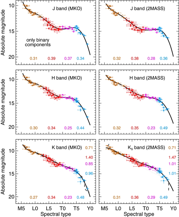
Figure 32. Same as Figure 25, but showing only components of binaries, with pairs connected by thin gray lines. The polynomial fits displayed are derived from the full data set (i.e., the data in Figure 25); they are not a fit to the data points plotted here.
Download figure:
Standard image High-resolution imageIf instead we gauge the brightening effect relative to the brightest object in the L/T transition, 2MASS J0559−1404 (T4.5, MJ = 13.49 ± 0.06 mag), these values would be ≈0.7 mag larger. This object is discussed in Section 6.2, where we find that its near- and mid-IR magnitudes are unlikely to be consistent with a pronounced brightening due to unusual cloud properties. Rather, the simplest explanation is that this object is an unresolved, nearly equal-flux binary, and thus its photometry should not be used to assess the J-band bump. The next brightest object in the L/T transition is SDSS J0000+2554 (T4.5, MJ = 13.98 ± 0.08 mag).
Note that previous studies have referred to the "amplitude" of the J-band brightening, with this term being used loosely (Dahn et al. 2002; Tinney et al. 2003; Vrba et al. 2004). This lack of specificity was appropriate, given the small sample of transition objects—the description of the phenomenon was largely based on the outstanding object 2MASS J0559−1404, which was ∼1 mag brighter compared to the late-L and mid/late-T dwarfs in those earlier studies. With larger parallax samples now available, some care is warranted when using this description. In particular, the cited amplitude of the brightening sometimes comes from comparing the brightest mid-T dwarfs with low-order polynomial fits to the absolute magnitudes for L and T dwarfs (Looper et al. 2008; Burgasser et al. 2010). Since polynomial fits are a convenient, but nonphysical, model for the large changes in magnitude as a function of spectral type, they inevitably do not provide a good match to all the data and serve to artificially enhance the outlier nature of the ≈T3–T4 objects. Thus, benchmarking the J-band behavior against polynomial fits should now be superseded by a direct comparison of measured absolute magnitudes as a function of spectral type (Tables 15 and 16; Figure 29).
7.1.2. Near-infrared Color–Magnitude Diagrams
Perhaps the most natural representation of the L/T transition can be found in near-IR CMDs (Figures 33 and 34). Here, the view of the transition is much clearer, as the large change in near-IR colors over a small range in spectral type is displayed with a long horizontal extent in the CMD. Objects in the J-band bump appear as the brightest objects in the blue vertical locus of the mid/late-T dwarfs, with 2MASS J0559−1404 being the most protruding object.

Figure 33. Color–magnitude diagrams in the MKO system showing binary components (large colored symbols) zoomed in on the L/T transition. The majority of data points here (72%) use our new CFHT parallaxes, and even more rely on our Keck resolved photometry. Thin gray lines connect binary pairs, and symbols are the same as Figure 16 for binary components. Open symbols indicate data where a flux ratio was estimated from spectral decomposition constrained by flux ratios measured in other bands. For one binary (SDSS J0805+4812), no symbol indicates that the flux ratio was not measured in any band, so resolved photometry is based solely on spectral decomposition. Smaller gray points show the locus of likely single objects (i.e., those unresolved in HST/AO imaging), only those with <0.10 mag errors for clarity.
Download figure:
Standard image High-resolution image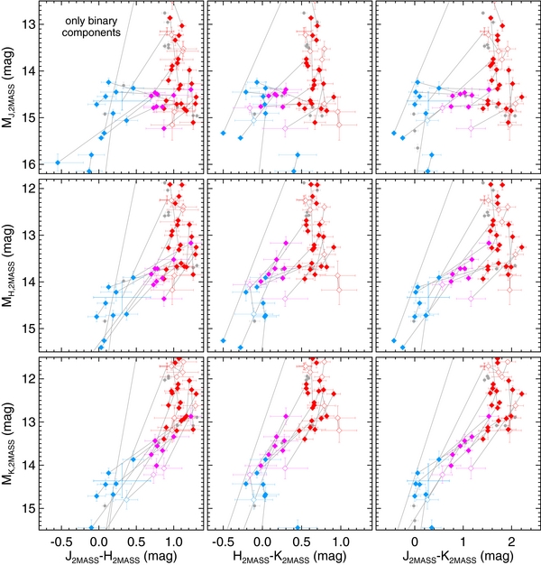
Figure 34. Same as Figure 33 but with photometry in the 2MASS system.
Download figure:
Standard image High-resolution imageFigures 33 and 34 show the CMDs assembled from resolved binary components, focusing on the L/T transition region. The distribution of the components is in accord with the CMD of the entire sample of objects, suggesting that unresolved binarity is not a significant issue for the latter. With this much larger sample of objects compared to previous work, one new feature appears: there is a "gap" in the color distribution in the transition, with many fewer objects seen with (J − H)MKO ≈ 0.1–0.3 mag and (J − K)MKO ≈ 0.0–0.4 mag as compared to redder (early-T and late-L) or bluer (mid-T) objects. There is no corresponding gap in H − K, and thus the above ranges in color appear to due almost entirely to changes in the J-band flux at fixed H − K color. (However, note that there appears to be a separate, much less prominent gap in H − K color just blueward of the red L dwarf sequence.) Since the density of objects in the CMD is related to the lifetimes of the various evolutionary phases, the natural interpretation is that the gap reflects the shortest lived phase of the L/T transition, shorter than the hotter or cooler stages. We also note that this gap appears when simply plotting the weighted averages of magnitudes binned by spectral type (Figure 30).
To highlight the gap, Figure 35 shows the histogram of near-IR colors for the range of absolute magnitudes representative of the L/T transition. In addition to the L/T gap, these plots also suggest a pileup of objects redward of the gap. This finding is highly evocative of work by Saumon & Marley (2008). They combine evolutionary models with dusty model atmospheres to simulate the distribution of objects in the near-IR CMD. To model the L/T transition, they build a "hybrid" prescription that combines the hotter dusty atmospheres with the cooler dustless ones, by linearly interpolating the surface boundary conditions in the model atmospheres from 1400 K to 1200 K. Such an approach produces a pileup of objects in this transition temperature range (see their Figure 13), as the hotter dusty objects must release more energy to transform into a cooler dust-free object than compared to objects which do not change cloud properties. Their simulated CMD shows a pileup of L/T objects at (J − K)MKO ≈ 1.0 mag, which they discuss extensively, and a relative paucity of objects at (J − K)MKO ≈ 0.2–0.6 mag, which they do not discuss. While the model-predicted colors of these features may not exactly match our data, the qualitative agreement is compelling. Our binary component CMDs suggest a prolonged stage of brown dwarf color evolution during which condensate clouds slowly dissipate before rapidly transitioning to bluer near-IR colors in the last stages of condensate removal. Although the CMDs most directly probe the color evolution of brown dwarfs (i.e., cloud dispersal), in the theoretical perspective of Saumon & Marley (2008) this pileup and gap are inextricably tied to luminosity evolution as well.
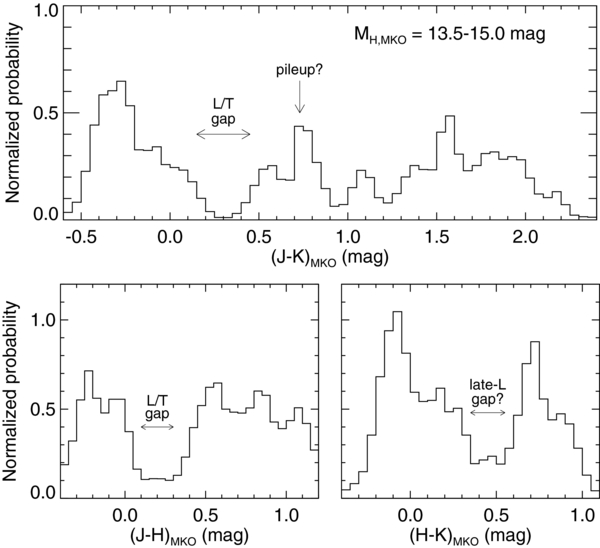
Figure 35. Distributions of near-IR colors for objects in the L/T transition, as selected by absolute magnitude (MH, MKO = 13.5–15.0 mag). Histograms were computed in a Monte Carlo fashion accounting for errors in colors and absolute magnitudes. The most prominent feature seen in near-IR CMDs (Figures 16 and 33) is a gap in (J − H)MKO and (J − K)MKO colors just blueward of the late-L/early-T dwarf sequence. This feature is clear in these histograms (labeled "L/T gap" here), and other features less obvious to the eye in the CMDs also appear. There is a less prominent gap in (H − K)MKO just blueward of the red L dwarf peak (labeled "late-L gap?") and an enhanced number of objects with (J − K)MKO = 0.5–0.9 mag (labeled "pileup?"). The L/T gap and the pileup are qualitatively similar to the behavior of near-IR colors along the L/T transition in the hybrid evolutionary models of Saumon & Marley (2008). In these models, brown dwarf evolution slows as a direct consequence of the removal of condensate cloud opacity across the L/T transition, resulting in a pileup of objects in J − K and a gap just blueward of this (though the particular colors of these features differ between their models and the data shown here).
Download figure:
Standard image High-resolution imageSince our collection of binary components is not a rigorously defined sample (e.g., volume-limited or magnitude-limited), selection effects are a natural concern but seem unlikely to fundamentally alter the outcome. The target lists for previous high angular resolution searches for ultracool binaries were derived primarily from three magnitude-limited searches: the SDSS ultracool dwarf search (e.g., Knapp et al. 2004; Chiu et al. 2006), the 2MASS L dwarf search (e.g., Cruz et al. 2007; Reid et al. 2008b), and the 2MASS T dwarf search (e.g., Burgasser et al. 2004). The 2MASS searches were based on near-IR color criteria that were inevitably incomplete from the latest L dwarfs to the mid-T dwarfs (≈L7–T5), while the SDSS search was based on far-red optical colors and thus sensitive to the full range of L and T dwarfs. (In fact, most of the objects redward of the J-band gap are from SDSS.) Moreover, it would be highly contrived to imagine a selection bias whereby integrated-light measurements of binaries containing a (J − H)MKO ≈ 0.2 component are avoided, while binaries with somewhat redder or bluer components are selected, especially as absolute magnitudes are relatively constant as a function of color across the transition. Thus, we conclude the "L/T gap" is real, though more rigorous samples are needed to quantify the relative numbers of bluer and redder objects straddling the gap. The parallax-based census possible with upcoming all-sky surveys like Pan-STARRS and LSST offer the most robust means of achieving this goal.
7.2. Individual L/T Binaries of Interest
A few objects warrant discussion based on the comparison of our results with previous work.
- 1.SDSS J0423−0414AB (T0 integrated-light near-IR type). Burgasser et al. (2010) decompose the integrated-light spectra based on the Burgasser et al. (2005b) HST/NICMOS F110W and F170M resolved photometry and find ΔK = 1.13 ± 0.07 mag, in excellent agreement with our observed ΔK = 1.18 ± 0.08 mag from Keck LGS AO.
- 2.SDSS J1021−0304AB (T3 integrated-light near-IR type). Burgasser et al. (2006c) resolved this system into a binary with HST/NICMOS and based on spectral decomposition suggested it shows a J-band flux inversion. This is seen for the first time with our Keck LGS AO data, making this the fourth system to show a flux inversion after 2MASS J1728+3948 (see below), SDSS J1534+1615, and 2MASS J1404−3159. More recent spectral decomposition by Burgasser et al. (2010) derives J- and K-band flux ratios of 0.16 ± 0.41 mag (i.e., no brightening) and 1.46 ± 0.29 mag, respectively. Within the large fitting uncertainties, this is consistent with our LGS AO measurements of −0.10 ± 0.03 mag (i.e., a J-band flux reversal) and 1.00 ± 0.03 mag.
- 3.2MASS J1404−3159AB (T3 integrated-light near-IR type). Looper et al. (2008) published this object as a binary using the same Keck data as presented here. Our flux ratio measurements are consistent with theirs within the quoted errors. Our uncertainties are a factor of 2–4 times smaller, which likely stems from the different analysis methods. The key differences are that Looper et al. (2008) manually adjust their image subtractions, use aperture photometry, and choose PSF reference stars that do not necessarily match the science data.
- 4.2MASS J1728+3948AB (L7 integrated-light optical type). Gizis et al. (2003) identified this system as a binary from HST/WFPC2 optical far-red imaging. This was the first known ultracool binary to show an inversion in its flux ratios with wavelength, where the earlier type component (identified as being the optically bluer object) was brighter in F814W but fainter in F1042M. Interestingly, our Keck LGS AO J-band imaging shows no inversion in the JHK flux ratios, indicating the wavelength-dependent behavior of the brightening can be rather complex. (This assumes variability effects between the non-simultaneous HST and Keck data are negligible.) To date, this binary is the only one with direct evidence for the brightening phenomenon extending as blue as 1 μm, though spectral decomposition suggests this occurs in other binaries (e.g., Figures 13–15, and also see Burgasser et al. 2010).
- 5.SDSS J2052−1609AB (T1 integrated-light near-IR type). This object was identified as a weak candidate for binarity by Burgasser et al. (2010) based on spectral decomposition and subsequently resolved by Stumpf et al. (2011) with VLT NACO in 2009. We present here an independent identification of this binary, obtained almost 4 years earlier in 2005. The flux ratios in J and K bands are consistent between VLT and Keck, but the H-band flux ratio appears to have changed from 0.33 ± 0.07 mag in 2005 to 0.57 ± 0.01 mag in 2009.
8. CONCLUSIONS
We present here the first results from our ongoing high-precision infrared astrometry program at CFHT targeting ultracool dwarfs (M6 to >T9). We have found that CFHT/WIRCam offers an excellent platform for measuring parallaxes to ultracool objects, given its relatively large aperture and the excellent seeing on Mauna Kea. Queue scheduling at CFHT is also a major advantage, as it enables good parallax phase coverage for targets widely distributed on the sky with almost no impact from poor weather. Queue mode also allows data to be obtained only during the times of best seeing while also following rigorous airmass constraints to eliminate the effects of DCR. The work we present here is the first to use CFHT/WIRCam for precision astrometry.
Using CFHT/WIRCam data collected since 2007, we have measured parallaxes for 34 binaries and 15 single objects (i.e., 83 objects in 49 systems) to a median precision of 1.1 mas (2.3%), and the best uncertainties are 0.7 mas (0.8%). For 48 objects in 29 systems we provide the first parallax measurements. For the 35 objects in 20 systems with published parallaxes we improve the precision in the vast majority of cases (29 objects in 17 systems). In these cases the median improvement in the published parallax error is a factor of 1.7, and as good as a factor of five. Comparison of targets in common between our program and published samples provides an independent check on our methods, and we generally find good agreement in parallax values. However, there are more >2σ outliers than is statistically expected, and Monte Carlo simulations for these objects reveal that this is likely because some published errors are underestimated by a factor of ≈2–3.
To enable detailed analysis of the complete sample of ultracool binaries with parallaxes, we also present here a large set of resolved near-IR photometry obtained with Keck AO imaging and aperture masking and archival HST and VLT data. Combining this photometry with near-IR spectroscopy from IRTF/SpeX, we determine component spectral types using a spectral decomposition technique. Unlike some previous studies, our method does not assume any relation between spectral type and absolute magnitude so that our resulting types may be used to assess this relationship. Our full sample comprises 17 M6–L1 dwarfs, 27 L1.5–L8 dwarfs, 22 L8.5–T5 dwarfs, and 17 ⩾T5.5 dwarfs. This doubles the number of L/T transition dwarfs with parallaxes and provides many high-precision distance measurements for ultracool binaries that will be crucial for future dynamical mass determinations.
These first results from our ongoing CFHT program provide high-precision parallaxes for a large sample of ultracool dwarfs, enabling some basic quantitative tests of brown dwarf evolution. We combine our sample of new or improved parallaxes for 74 objects with previously published parallaxes for a total sample of 314 objects that allows us to form an unprecedented view of the absolute magnitudes of ultracool dwarfs and provide an update of key empirical relations.
- 1.We determine empirical relations between absolute magnitude and spectral type for a wide variety of near- and mid-IR photometric systems (MKO, 2MASS, Spitzer/IRAC, and WISE). We compute simple polynomial fits to these relations but suggest that using the actual tabulated values of mean and rms absolute magnitude is preferred for quantitative analysis.
- 2.We are able to quantify the intrinsic scatter in absolute magnitude at a given spectral type with our high-precision parallaxes. As expected, this reveals relatively small intrinsic variations in the near-IR among late-M dwarfs (0.1–0.3 mag) that increases for L dwarfs (0.3–0.5 mag) as dust properties become an important "second parameter" after Teff. We also identify a large, previously unappreciated amount of intrinsic scatter among mid- to late-T dwarfs in the near-IR (0.3–0.8 mag), presumably due to metallicity and surface gravity variations in the field population.
- 3.We identify astrometric perturbations due to orbital motion in three targets: SDSS J0805+4812AB, previously suggested to be a binary based on its unusual spectrum; and the known binaries 2MASS J0518−2828AB (L6.5+T5) and 2MASS J1404−3159AB (L9+T5).
- 4.We find evidence for unresolved, nearly equal-flux binaries based on their overluminosity in near- and mid-IR CMDs and spectral-type–absolute-magnitude relations: 2MASS J0559−1404 (T4.5), which was previously known to be overluminous; SDSS J1504+1047 (T7), for which we measure a parallax for the first time; and SDSS J1021−0304A (T0 ± 1), which our 3.5× improved parallax precision reveals lies ≈0.5 mag above the L/T transition in near-IR CMDs and which is unusually bright for its spectral type. If SDSS J1021−0304A is indeed binary, it would be a member of a hierarchical triple with SDSS J1021−0304B (T5). This idea can be tested with a dynamical mass for the system in the near future.
- 5.Our parallax measurement for the wide pair SDSS J1416+1348 (L6) and ULAS J1416+1348 (T7.5p) shows that the components occupy unusual locations on near- and mid-IR CMDs. We conclude the system has lower metallicity than typical field dwarfs, with the possibility remaining that unusual cloud properties and high surface gravity could also be affecting the components' observed features.
- 6.We investigate the kinematics of all ultracool dwarfs with parallaxes, searching for wide common proper motion companions and deriving criteria for identifying likely thick disk or halo members based on large tangential velocities. We identify two new candidate wide companions, and find that one previously identified pair is likely to be a chance alignment based on our improved proper motion (2MASS J0850+1057AB and NLTT 20346AB). We do not identify any new thick disk or halo members.
- 7.We find no evidence for a spectral type "flip" in the components of 2MASS J0850+1057AB, as recently suggested by Burgasser et al. (2011). We find types of L6.5 ± 1 and L8.5 ± 1, in contrast to L7+L6 from their analysis, thereby making 2MASS J0850+1057A normal for its spectral type and thus requiring no special explanation such as youth or unresolved multiplicity.
- 8.We have increased the sample of resolved L/T systems having multi-band near-IR photometry and a measured parallax by more than a factor of three. We use these resolved components to provide the clearest view to date of the L/T transition. We find that the amplitude of the J-band brightening ("bump") is ≈0.5 mag, as defined by the mean absolute magnitude as a function of spectral type. As brown dwarfs cool they appear to reach a local minimum in J-band brightness at ≈L8. In the framework of current models, this would correspond to the maximal suppression of J-band flux due to high condensate opacity. As objects evolve from red to blue near-IR colors, the J-band flux increases, presumably due to cloud dissipation, reaching a local maximum in J-band flux at ≈T4.5. A similar pattern is seen in Y band, but perhaps with a larger amplitude of ≈0.7 mag. Brightening is not seen in the H, K, and L' bands, which instead are consistent with a monotonic decline as a function of spectral type. This behavior is consistent with flux ratios measured in near-IR bandpasses for binaries that span the L/T transition (e.g., Liu et al. 2006; Looper et al. 2008; Burgasser et al. 2010; Stumpf et al. 2011).
- 9.We find an apparent "gap" in the evolution of brown dwarfs as they traverse the L/T transition in near-IR CMDs at roughly constant absolute magnitude. There is a conspicuous paucity of objects over specific color ranges, (J − H)MKO ≈ 0.1–0.3 mag and (J − K)MKO ≈ 0.0–0.4 mag, with no gap in (H − K)MKO. Immediately redward of this gap is an apparent pileup of objects in (J − K)MKO color. This is highly evocative of the pileup and gap seen in the "hybrid" tracks of Saumon & Marley (2008), which self-consistently model brown dwarf evolution using a prescription for cloud dissipation at the L/T transition. Regardless of the exact cloud prescription, they suggest that there should always be a pileup of some kind because hotter dusty objects must release much more energy to become cooler dust-free objects compared to objects that do not change dust properties. (They do not discuss the subsequent gap, though it is apparent in their model CMDs.) The features we observe in the near-IR CMDs thus indicate a slowing of color evolution at the last stages of condensate cloud dissipation (possibly related to a slowing of luminosity evolution) before brown dwarfs rapidly transform to their final, dust-free, blue near-IR colors (≳T4.5).
The capability of measuring ≈1 mas parallaxes for faint infrared sources is novel. We have achieved the highest precision to date for such faint objects (J = 13.5–16.5 mag, and as faint as 19.7 mag at somewhat reduced precision). Although our precision goal has initially been driven by the need for high-quality dynamical masses, this new capability opens the door to other previously inaccessible samples. For example, rare classes of ultracool dwarfs are on average more distant and thus need high precision for useful parallaxes. In addition, the faintest ultracool dwarfs known (J ≳ 18 mag) are beyond the reach of previous parallax programs but can be efficiently monitored with CFHT. Such new samples will be the subject of our future publications.
We are deeply indebted to the CFHT staff for their constant observing support and dedication to delivering the highest quality data products, and in particular to Loic Albert. We also thank Brendan P. Bowler, Kimberly Aller, and Mark Pitts for assistance in conducting our IRTF/SpeX observations. We are grateful to S. K. Leggett and Michael J. Ireland for suggestions that significantly improved our analysis. We have benefited from discussions with Jan Kleyna, Gene Magnier, Dave Monet, John Thorstenen, Chris Tinney, John Tonry, and Fred Vrba about astrometry and parallaxes. We are grateful to Céline Reylé for customized Besançon Galaxy models. It is a pleasure to thank Joel Aycock, Randy Campbell, Al Conrad, Heather Hershley, Jim Lyke, Jason McIlroy, Gary Punawai, Julie Riviera, Hien Tran, Cynthia Wilburn, and the Keck Observatory staff for assistance with the Keck observations. Our research has employed the 2MASS data products; NASA's Astrophysical Data System; the SIMBAD database operated at CDS, Strasbourg, France; and the SpeX Prism Spectral Libraries, maintained by Adam Burgasser at http://www.browndwarfs.org/spexprism. This publication makes use of data products from the Wide-field Infrared Survey Explorer, which is a joint project of the University of California, Los Angeles, and the Jet Propulsion Laboratory/California Institute of Technology, funded by the National Aeronautics and Space Administration. This research has made use of the NASA/IPAC Infrared Science Archive, which is operated by the Jet Propulsion Laboratory, California Institute of Technology, under contract with the National Aeronautics and Space Administration. This publication has made use of a contour plotting code written by James R. A. Davenport. T.J.D. and M.C.L. acknowledge support for this work from NSF grants AST-0507833 and AST-0909222. M.C.L. acknowledges support from an Alfred P. Sloan Research Fellowship. T.J.D. acknowledges support from Hubble Fellowship grant HST-HF-51271.01-A awarded by the Space Telescope Science Institute, which is operated by AURA for NASA, under contract NAS 5-26555. Finally, the authors wish to recognize and acknowledge the very significant cultural role and reverence that the summit of Mauna Kea has always had within the indigenous Hawaiian community. We are most fortunate to have the opportunity to conduct observations from this mountain.
Facilities: Keck:II (LGS AO, NIRC2) - KECK II Telescope, CFHT (WIRCam) - Canada-France-Hawaii Telescope, IRTF (SpeX) - Infrared Telescope Facility, Spitzer (IRAC) - Spitzer Space Telescope satellite, WISE - Wide-field Infrared Survey Explorer
Footnotes
- *
Based on observations obtained with WIRCam, a joint project of CFHT, Taiwan, Korea, Canada, France, at the Canada–France–Hawaii Telescope (CFHT) which is operated by the National Research Council (NRC) of Canada, the Institute National des Sciences de l'Univers of the Centre National de la Recherche Scientifique of France, and the University of Hawaii.
- †
Some of the data presented herein were obtained at the W. M. Keck Observatory, which is operated as a scientific partnership among the California Institute of Technology, the University of California, and the National Aeronautics and Space Administration. The Observatory was made possible by the generous financial support of the W. M. Keck Foundation.
- 4
- 5
http://www.browndwarfs.org/spexprism, maintained by Adam Burgasser.
- 6
S/N
. - 7
We emphasize that while our dither registration is done in celestial coordinates, the output relative positions are deliberately not tied to an absolute reference frame. This is because most astrometric catalogs have a lower precision than our measurements and would unnecessarily introduce systematic errors into the relative measurements at this stage. Our initial catalog match provides only the approximate field coordinates, to within ≈1'', which is needed to achieve an accurate tangent projection and match our measured positions to an absolute reference catalog at a later step (Section 2.3).
- 8
The small number of galaxies among our reference sources is both supported by the lack of extended sources and expected from galaxy count measurements. For our typical exposure time of 5 s, our high S/N reference sources are brighter than J of 17 mag. Cristóbal-Hornillos et al. (2009) predict 500 galaxies deg−2 with J < 17 mag, and for the 0.028 deg2 field of view of one WIRCam detector, this implies 14 galaxies. This is much smaller than the ≈40–200 reference stars in our fields (see Table 3). In fact, given that galaxies have larger FWHM they will have a larger rms in their position measurement, and thus most will be excluded by our rms cuts at the beginning of the epoch-matching step.
- 9
All spectral decomposition methods effectively assume that the templates being used are accurate representations of a single object of that spectral type. This is most important around the L/T transition as a blended L+T dwarf spectrum can show significant anomalies relative to single objects (e.g., Cruz et al. 2004). The templates we used have been cleaned of all known binaries, as well as the six strong spectral blend binary candidates proposed by Burgasser et al. (2010).
- 10
- 11
Although it formally passes our selection criteria for plotting, we exclude the young L dwarf AB Pic b from the CMD figures. The exceptionally red (J − H)2MASS and (J − K)2MASS colors (1.37 mag and 2.02 mag, respectively) make this object an unusually prominent outlier in the CMDs, being ≈0.4–0.5 mag redder than objects of comparable absolute magnitude or spectral type. While this may reflect a unique SED for this source, another possibility is that the J-band photometry uncertainty is larger than reported. This speculation is supported by two possible pieces of evidence. (1) Figure 6 of Wahhaj et al. (2011) shows that the J − H color of AB Pic b is far redder than all other known young companions and field ultracool dwarfs, but not its H − K color. (2) Bonnefoy et al. (2010) show that the near-IR spectra of AB Pic b in the individual J, H, and K bandpasses are consistent with previously known young early-L dwarfs. But if the published JHK photometry is used to assemble a flux-calibrated SED, the resulting near-IR spectrum has a very peculiar broadband appearance (B. Bowler 2011, private communication). Thus we conservatively choose to exclude AB Pic b from the CMD plots.
- 12
Burgasser et al. (2008b) determined that 2MASS J0939−2448 is overluminous for its model atmosphere derived temperature, concluding that it was likely an unresolved, nearly equal-flux binary. This conclusion was also reached by Leggett et al. (2009) from analysis based on model atmospheres. Our interpretation does not necessarily require unresolved binarity to explain the observations since we find that 2MASS J0939−2448 is unusual in color rather than in magnitude. If single, the model-derived Teff from previous work would be systematically offset from the actual Teff, possibly due to this object's subsolar metallicity and/or high gravity.
- 13
Note that the updated parallax from Schilbach et al. (2009) for 2MASS J0532+8246 decreases its distance by 2σ (13%), resulting in normal mid-IR magnitudes.
- 14
The only ultracool binaries wider than SDSS J1416+1348AB are pairs with late-M primaries: 2MASS J01303563−4445411AB (M9+L6:, 130 ± 50 AU; Dhital et al. 2011); DENIS-P J055146.0−443412AB (M8.5+L0, 250 ± 50 AU; Billères et al. 2005); Koenigstuhl 1 (M6:+M9.5, 1800 ± 170 AU; Caballero 2007b); 2MASS J01265549−5022388AB (M6.5+M8, 5100 ± 400 AU; Artigau et al. 2007); and 2MASS J12583501+4013083AB (M6:+M7:, 6700 ± 800 AU; Radigan et al. 2009). Note that the values listed here are projected separations.
- 15
Note that these comparisons assume negligible near-IR variability, which is actually unknown for these specific objects but which is generally found to be ≲0.05 mag for objects of similar spectral type (Koen et al. 2004, 2005; Clarke et al. 2008; Artigau et al. 2009). Thus, variability is expected to have a negligible impact in our analysis since it is comparable to or much smaller than the uncertainties in the colors and absolute magnitudes. In addition, Radigan et al. (2012) find that the colors of variable ultracool dwarfs stay relatively constant while it is their overall flux that increases and decreases, so variability should have an even smaller impact on our noncontemporaneous color comparisons.
- 16
The decomposition of 2MASS J0518−2828AB by Cruz et al. (2004) used the spectrum of SDSS J1021−0304AB as a template, which was later found to be a binary (Burgasser et al. 2006c). The latest decomposition presented here (Figure 13) suggests no flux reversal between the components, which is also consistent with the results from Burgasser et al. (2010).
