


ABSTRACT
We describe a new Godunov algorithm for relativistic magnetohydrodynamics (RMHD) that combines a simple, unsplit second-order accurate integrator with the constrained transport (CT) method for enforcing the solenoidal constraint on the magnetic field. A variety of approximate Riemann solvers are implemented to compute the fluxes of the conserved variables. The methods are tested with a comprehensive suite of multi-dimensional problems. These tests have helped us develop a hierarchy of correction steps that are applied when the integration algorithm predicts unphysical states due to errors in the fluxes, or errors in the inversion between conserved and primitive variables. Although used exceedingly rarely, these corrections dramatically improve the stability of the algorithm. We present preliminary results from the application of these algorithms to two problems in RMHD: the propagation of supersonic magnetized jets and the amplification of magnetic field by turbulence driven by the relativistic Kelvin–Helmholtz instability (KHI). Both of these applications reveal important differences between the results computed with Riemann solvers that adopt different approximations for the fluxes. For example, we show that the use of Riemann solvers that include both contact and rotational discontinuities can increase the strength of the magnetic field within the cocoon by a factor of 10 in simulations of RMHD jets and can increase the spectral resolution of three-dimensional RMHD turbulence driven by the KHI by a factor of two. This increase in accuracy far outweighs the associated increase in computational cost. Our RMHD scheme is publicly available as part of the Athena code.
1. INTRODUCTION
A study of the properties and behavior of magnetized fluids in the relativistic limit is increasingly important for a wide variety of astrophysical problems, such as accretion flows close to the event horizon of a black hole (Beckwith et al. 2008), gamma-ray bursts (Morsony et al. 2007), and blazar jets (Begelman 1998) to name but three. Often the inherent nonlinearity of the underlying equations and the need to account for multi-dimensional effects mean that only limited insight can be gained from purely analytic studies. As a result, there is a clear need for the development of numerical algorithms to solve the equations of relativistic magnetohydrodynamics (RMHD) in multi-dimensions. Although algorithms based on operator splitting have been very successful when applied to RMHD (e.g., De Villiers & Hawley 2003), in the past decade there has been considerable effort devoted to the extension of Godunov methods to RMHD, beginning with Komissarov (1999a) and including, for example, Balsara (2001), Gammie et al. (2003), Leismann et al. (2005), Noble et al. (2006), Del Zanna et al. (2007), Mignone & Bodo (2006), and Mignone et al. (2009). Such methods have the advantage of not requiring an artificial viscosity for shock capturing, and since they adopt the conservative form, the coupling between the total energy and momentum inherent in relativistic flow is preserved directly.
In this paper, we describe a new Godunov scheme for RMHD. There are two critical ingredients to this algorithm which distinguish it from previous work. First and foremost is the method by which the divergence-free constraint is enforced on the magnetic field. Our algorithm combines the staggered, face-centered field version of the constrained transport (CT) algorithm with the method of Gardiner & Stone (2005, 2008) to compute the electric fields at cell edges. This allows the cell-centered, volume-averaged discretization of the divergence to be kept zero to machine precision. Because of the tight coupling between the conserved variables in RMHD, enforcing the divergence-free constraint through the integration algorithm using CT is likely to offer advantages over post facto fixes to the field provided by divergence cleaning methods (Anninos et al. 2005; Mignone et al. 2010).
The second crucial ingredient to our algorithm is the use of a dimensionally unsplit integrator. Algorithms for MHD based on dimensional splitting require source terms that break the conservative form (Powell et al. 1999). Thus, in this work we adopt the MUSCL-Hancock integrator described by Stone & Gardiner (2009), hereafter we refer to the combination of this integrator and CT as the "VL+CT" algorithm. The VL+CT integrator is particularly well suited to RMHD as it does not require a characteristic decomposition of the equations of motion in the primitive variables, which in RMHD is extremely complex (see Antón et al. 2010), nor does it require the various source terms necessary for the integration of the MHD equations in multi-dimensions that are required for the Corner Transport Upwind + Constrained Transport ("CTU+CT") integrator described in Gardiner & Stone (2005, 2008). Previous experiments (such as supersonic MHD turbulence; Lemaster & Stone 2009) have shown this integrator to be more robust with only a small increase in diffusivity compared to CTU+CT.
In addition to these two ingredients, other important aspects of the algorithm described here are the choice of the Riemann solver used to compute the fluxes of the conserved variables at cell edges and the method by which the pressure and velocity (the "primitive" variables) are recovered from the total energy and momentum (the "conserved" variables). We have implemented and tested a variety of exact and approximate Riemann solvers for relativistic hydrodynamics and RMHD, and we provide comparison of the accuracy and fidelity of each on multidimensional applications in this paper. To convert the conserved into the primitive variables, we adopt the 1 DW approach of Noble et al. (2006), implemented as described by Mignone & McKinney (2007) with some minor modifications. Both the Riemann solvers and inversion algorithm are described in more detail in the following sections.
It is generally appreciated that numerical algorithms for RMHD are more complex and less robust than similar methods for Newtonian MHD, primarily because of the nonlinear couplings between the conserved and primitive variables and the possibility of unphysical fluxes or superluminal velocities in approximate Riemann solvers. We have developed a hierarchy of correction steps to control errors introduced by these challenging aspects of the algorithm, ranging from the use of less accurate but more robust Riemann solvers to compute the fluxes, to the use of a first-order algorithm to integrate individual problematic cells, and to the use of approximate inversion algorithms that break conservation when all else fails. While these corrections are required exceedingly rarely (in less than one in 109 cell updates in the most challenging cases), they are crucial for improving the stability of the algorithm. We document all of our strategies in this paper with the expectation that some of them must be useful in other codes as well.
This paper also presents a series of multi-dimensional tests for RMHD which have solutions that illustrate important properties of the numerical method, such as its ability to hold symmetry or to test that the solenoidal constraint is preserved on the correct stencil. Although one-dimensional test suites (e.g., Komissarov 1999a; Balsara 2001; De Villiers & Hawley 2003) are useful for developing various elements of numerical algorithms for RMHD, we have found that multi-dimensional tests are far more exacting because they require that the tight couplings between components of four vectors are handled with minimal errors, and they test whether the scheme is free of pathologies related to, for example, violations of the solenoidal constraint on the magnetic field.
Our algorithms for RMHD have been implemented within the Athena code for astrophysical MHD (Stone et al. 2008). For this reason, it can use features of the code that were originally developed for Newtonian MHD, such as static mesh refinement (SMR). The code is freely available (with documentation) for download from the Web.3
The remainder of this paper is structured as follows. In Section 2, we develop the equations of RMHD into a form suitable for numerical integration. In Section 3, we describe the details of our algorithm, including (1) the primitive variable inversion scheme, (2) the various Riemann solvers we use for RMHD, (3) our method for reconstructing the left and right states at cell interfaces, (4) our methods for correcting unphysical states, (5) the steps in the unsplit integration algorithm, and (6) the extension of the SMR algorithm in Athena to RMHD. In Section 4, we give the details and results of the tests we have developed for multi-dimensional RMHD, while in Section 5 we describe some preliminary applications of the algorithm, using SMR, to two problems: the propagation of supersonic jets and the development of turbulence and magnetic field amplification in the Kelvin–Helmholtz instability (KHI). Finally, in Section 6, we summarize the work and point to future directions of research.
2. THEORETICAL BACKGROUND
2.1. Equations of RMHD
The evolution of a relativistic, magnetized plasma is governed by the conservation laws for particle number,

and stress energy,

The evolution of the electromagnetic field is described by Maxwell's equations,

supplemented by the equation of charge conservation,

In the above, ρ is the mass density measured in the comoving frame, Uμ is the four-velocity (which is subject to the constraint UμUμ = −1), Tμν is the stress-energy tensor, Jν is the four-current density, Fμν is the antisymmetric electromagnetic field tensor with its dual. The latter two are related to the electric, , and magnetic, , fields through


where  μναβ is the contravariant form of the Levi-Civita tensor and nν is a future-pointing, time-like unit vector. We adopt units with c = 1 and adopt the usual convention that Greek indices run from 0 to 3 and are used in covariant expressions involving four-vectors and that latin indices run from 1 to 3 and are used to denote components of three-vectors. We adopt Lorentz–Heaviside notation for the electromagnetic fields so that factors of are removed. We work in a spatially flat, Cartesian coordinate system such that the line element, ds2, and the metric tensor, gαβ, are given by


In this coordinate system, the divergence of a four-vector and tensor are given by

respectively.
We now use this set of conventions to transform the conservation laws and Maxwell's Equations (1)–(3) into a form suitable for numerical integration. We begin with Maxwell's equations and work in the ideal MHD limit such that in the fluid rest frame, the Lorentz force on a charged particle is zero, FμνUν = 0. Splitting the second of Equation (3) into its temporal and spatial components and exploiting the antisymmetry of yield a constraint and an evolution equation,


Substituting the definition of the electromagnetic field strength tensor and its dual (Equation (5)) into the second of Maxwell's equations and using the ideal MHD conditions yield

Here, Vi = Ui/Γ is the velocity three-vector ("transport" velocity) and Γ = (1 − |V|2)−1/2 is the Lorentz factor. Note that we can write the velocity four-vector as , the electric field four-vector as and the magnetic field four-vector as . In terms of the three-vectors, , the above equations take the form


These are the solenoidal constraint, induction equation, and ideal MHD condition familiar from Newtonian MHD. To arrive at an equation describing the evolution of the momentum and total energy of the fluid, we begin by recalling that the stress-energy tensor can be decomposed into components describing the fluid,

and the electromagnetic field (see, e.g., Jackson 1975):

Here, δμν is the Kronecker-delta symbol, h is the relativistic enthalpy, and Pg is the gas pressure. Throughout the remainder of this work, we will assume an ideal gas equation of state, such that

where γ is the adiabatic exponent (constant specific heat ratio).
A simple expression for the stress-energy tensor of the electromagnetic field can be obtained by introducing the magnetic field four-vector:

Expanding Equation (14), substituting the definitions for the velocity three-vectors, and using the ideal MHD condition yield

The stress-energy tensor for the electromagnetic field in ideal MHD then takes the form (see, e.g., De Villiers & Hawley 2003)

In this notation, conservation of stress energy is therefore expressed through

Finally, applying the identities for the divergence of a four-vector and tensor given in Equation (7) yields

This system of conservation laws can be cast in a standard form used for numerical integration by defining vectors of conserved and primitive variables, U and W, respectively,

We can express the conserved variables, U, in terms of the primitive variables, W, by making use of the definitions of , yielding


Unfortunately, unlike the Newtonian case, analytic expressions for W(U) are not available and instead W must be obtained numerically. Our implementation of the required procedure is described in Section 3.1.
Defining a vector of fluxes in the x-direction, F(U), as

where we have utilized the ideal MHD constraint, , in order to write, for example, , we can write the system of conservation laws (Equation (18)) in the standard form:


where expressions for G(U) and H(U) can be found from F(U) by cyclic permutation of indices.
2.2. Spatial and Temporal Discretization
The system of conservation laws (Equation (22)) is integrated on a uniform Cartesian grid of dimensions Lx, Ly, Lz, which is divided into nx, ny, nz cells such that δx = Lx/nx and similarly for δy, δz. A cell centered at position (xi, yj, zk) is denoted by indices (i, j, k). Similarly, time in the interval t ∈ (t0, tf) is divided into N uniform steps, determined by the requirement that a wave traveling at the speed of light, c = 1 crosses a fraction of a grid cell determined by the Courant number, C, that is

Here, C is determined from the stability requirements of the algorithm, which for the second-order accurate VL+CT integrator adopted here is C ⩽ 0.5.
Conservation of mass (measured in the lab frame), D, momentum, Mk, and energy, E are treated using a finite-volume discretization such that these quantities are regarded as an average over the cell volume, δxδyδz,

while the associated fluxes are the time- and area-averaged flux through the face of the cell,

These quantities are then updated according to, for example,

The induction equation is integrated using a finite-area discretization such that the magnetic field three-vector, , is regarded as an area average over the surface of the cell,


while the associated electromotive forces (emfs) that are averaged along the appropriate line element are

The magnetic field is then updated according to, for example,

There are therefore two sets of magnetic field three-vectors utilized in this scheme, the face-centered, surface-area-averaged fields which are updated using CT, and a set of cell-centered, volume-averaged fields, which are computed using second-order accurate averages, for example,


The face-centered fields are always regarded as the primary representation of the magnetic field.
3. NUMERICAL METHOD
3.1. Primitive Variable Inversion
Many of the elements developed for numerical schemes for Newtonian MHD carry across directly to the relativistic case. The major exception to this is the method by which the vector of primitive variables, W, is recovered from the vector of conservative variables, U. In Newtonian physics, there are simple algebraic relationships between these two sets of quantities so that one can express W(U) analytically. Unfortunately, this is not the case in relativistic MHD and as a result, the method by which the primitive variables are recovered from conserved quantities lies at the heart of any numerical scheme. Detailed examination of a variety of methods to accomplish this procedure are presented in Noble et al. (2006). Our chosen method corresponds to the 1 DW scheme described by these authors, implemented as described by Mignone & McKinney (2007) with the modification that we use the total energy, E, as one of our conserved quantities rather than the difference of the total energy and the rest mass, E − D. We take this approach for the sake of simplicity and for compatibility with the SMR algorithm detailed in Section 3.6. The algorithm implemented within Athena is compatible with the equation of state for an ideal gas; extension to more general equations of state can be accomplished by modification of this algorithm as described by, e.g., Mignone & McKinney (2007) for the Synge gas. We give a brief overview of the details of our method below; the interested reader is referred to the above references for further details.
In our version of the scheme described by Mignone & McKinney (2007), the primitive variables, W, are found by finding the root of a single nonlinear equation in the variable Q = ρhΓ2:

which arises directly from the definition of the total energy, E (see Equation (20)). Here, and the remaining unknowns, Pg, Γ, can be written in terms of Q via


Finding the root of Equation (31) is accomplished via a Newton–Raphson (NR) iteration scheme (see, e.g., Press et al. 1992) for which it is necessary to supply derivatives of f(Q) with respect to Q:

where

The NR root finder requires an initial guess for the independent variable, W. This is obtained in a similar fashion to that described in Mignone & McKinney (2007) by finding the positive root of the quadratic equation

which guarantees a positive initial guess for the pressure, Pg. The ability to accurately predict an initial guess for the NR iterations is a major advantage to this scheme because it means values for the primitive variables from the previous time step do not need to be saved for use as the first guess. This results in a significantly simplified code structure, particularly with regard to implementation of algorithms for SMR (see Section 3.6). Once f(Q) = 0 has been determined within some desired tolerance (typical ∼10−10), the velocity three-vector, Vi, is determined via

3.2. Computing the Interface States
The conserved variables to the left, ULi−1/2, and right, URi−1/2, of the cell interface at i − 1/2 are reconstructed from cell-centered values using second-order accurate piecewise linear interpolation as described in Section 4.2 of Stone & Gardiner (2009) with two important differences. First, we perform limiting solely on the primitive variables, W, rather than the characteristic variables. Second, we replace the velocity three-vector contained in the primitive state, W, at the cell centers with the four-velocity, Uμ, and then recalculate the three-velocity based on the reconstructed components of this four-vector at the cell interfaces. This procedure helps to ensure that reconstruction does not result in an unphysical primitive state, characterized in this case by |V|2>1, and is particularly important for strongly relativistic shocks (for example, the Γ = 30 colliding shock described in Mignone & Bodo 2006). In the case where reconstruction does result in an unphysical primitive state, we revert to first-order spatial reconstruction. We note that the scheme can easily be extended to third-order spatial accuracy by implementation of, for example, the Piecewise Parabolic Method of Colella & Woodward (1984). We note though that improving the order of convergence of the reconstruction algorithm is not always the best approach to improve the overall accuracy of the solution as demonstrated in Stone et al. (2008).
3.3. Riemann Solvers
Computation of the time- and area-averaged fluxes (e.g., Equation (25)) is accomplished via a Riemann solver, which provides the solution (either exact or approximate) to the initial value problem:

Here, UL,Ri−1/2 are the left and right states at the zone interface located at i − 1/2 computed in the reconstruction step described in Section 3.2. A variety of Riemann solvers of varying complexity can be used. To date, we have implemented three such solvers, all of which belong to the Harten–Lax–van Leer (HLL) family of nonlinear solvers. Approximate HLL-type solvers require knowledge of the outermost wave speeds of the Riemann fan, λL,R, which correspond to the fast magnetosonic waves. Accurate calculations of speed of these waves involve finding the roots of the quartic polynomial (Anile 1989):

where c2s = γPg/ρh is the sound speed. This quartic is solved by standard numerical techniques (see, e.g., Mignone & Bodo 2006), which we have found to provide an accurate solution for λ provided a physical state is input. The roots of the quartic are sorted to find the smallest, λ−, and largest, λ+, roots for both UL and UR. Finally, λL,Rare then found from Davis (1988):

We have found that the robustness of the code is greatly improved by using accurate calculations of the wave speed, rather than estimates based on quadratic approximations (as described in, for example, Gammie et al. 2003).
3.3.1. HLLE Solver
The simplest Riemann solver that we have implemented in Athena for RMHD is the HLLE solver (Harten et al. 1983), which computes the solution to Equation (37) as

where λL,R are the slowest, fastest wave speeds and Uhll is the state integral average of the solution of the Riemann problem (Toro 1999):

The interface flux associated with this solution is

where Fhll is the flux integral average of the solution of the Riemann problem:

Note that setting |λL| = |λR| = c = 1 reverts the interface fluxes defined above to the Lax–Friedrichs prescription, thereby applying maximal dissipation (which for RMHD is set by the speed of light) to the solution of the Riemann problem.
3.3.2. HLLC Solver
While the nonlinear HLLE solver described above provides a robust, simple, and computationally efficient method to calculate the upwind interface fluxes required for the solution of Equation (22), it has a major drawback in that contact and rotational discontinuities are diffused even when the fluid is at rest. Mignone & Bodo (2006) describe the extension of the nonlinear HLLC (HLL "contact," denoting the restoration of the contact discontinuity to the Riemann fan) solver (Toro 1999) to relativistic MHD and we have implemented this solver within Athena.
This is accomplished by the solution of the Rankine–Hugoniot jump conditions across the left- and right-going waves as well as across a contact wave intermediate between the two. This requires solving a single quadratic equation for the speed of the contact discontinuity and then using this quantity to solve the jump conditions across the left- and right-going waves for the intermediate states (further details can be found in Mignone & Bodo 2006). We have implemented this solver following the version in the publicly available Pluto code (Mignone et al. 2007), and we encourage the interested reader to refer to both this code and Athena for algorithmic details not found in Mignone & Bodo (2006). We have found that the HLLC solver involves little increase in cost or complexity compared to HLLE, while greatly increasing the accuracy of the resulting interface fluxes. However, the tests in Section 4 show that this solver does possess pathologies relating to separate treatments of the case where and , in addition to exhibiting singular behavior in the case where with or Vz ≠ 0 (i.e., for truly three-dimensional MHD flows); see the discussion in Section 3.3 of Mignone & Bodo (2006).


3.3.3. HLLD Solver
The shortcomings of the HLLC solver for truly three-dimensional MHD flows led Mignone et al. (2009) to extend the nonlinear HLLD solver (Miyoshi & Kusano 2005) to relativistic MHD. The name is chosen to indicate that both the contact and the rotational discontinuities are restored to the Riemann fan.
For this solver, the intermediate states and wave speeds are determined by the solution of the Rankine–Hugoniot jump conditions across the left- and right-going fast waves and left- and right-going rotational discontinuities (Alfvén waves), and then matching solutions are applied across the contact discontinuity. Unlike the case of Newtonian MHD, the solution to this problem admits discontinuities in the normal component of the velocity in the intermediate states due to the effects of relativistic aberration (see, e.g., Antón et al. 2010). Despite these complexities, the solution of the problem is determined matching the normal velocity associated with the states to the left and right of the contact discontinuity across this discontinuity, which amounts to solving a one-dimensional, nonlinear equation in the total pressure, accomplished by standard numerical techniques to a typical accuracy of ∼10−7 (further details can be found in Mignone et al. 2009). We have implemented this solver, again following the version in the publicly available Pluto code (Mignone et al. 2007), and we again encourage the interested reader to refer to both this code and Athena for algorithmic details not found in Mignone et al. (2009). The formulation of the HLLD solver removes the flux singularity suffered by the HLLC solver in the truly three-dimensional case, and as such we find that the HLLD solver is better suited than the HLLC for truly multi-dimensional MHD problems (Mignone et al. 2009).
3.4. When Everything Goes Wrong
The most significant challenge presented in extending a Newtonian integration algorithm to relativistic MHD is developing a strategy to resolve the case where the integration algorithm produces a conserved state, U, that does not correspond to a physical primitive state, W. Such a failure can take place in one of five different ways: first, the Godunov fluxes derived from the Riemann solver can be non-real valued; second, the algorithm outlined in Section 3.1 can fail to converge; third, the density can become negative, ρ < 0; fourth, the gas pressure can become negative, Pg < 0; and finally, the velocity can become superluminal, |V|2>1. To resolve the first of these failure modes, one can simply verify that the Godunov fluxes obtained from the Riemann solver are real valued and replace those that are not with a more diffusive estimate. For the remaining failure modes, several approaches are possible; for example, one can revert to a first-order update which applies enhanced numerical dissipation (derived from the Riemann solver) to the affected cells while retaining the conservative properties of the algorithm (see, e.g., Lemaster & Stone 2009). Alternatively, one can break the conservative properties of the algorithm and derive the gas pressure from the entropy, which guarantees the gas pressure to be positive definite (see, e.g., Noble et al. 2009). A third approach is to set the density and gas pressure to floor values and derive an estimate for |V|2 satisfying |V|2 < 1 (see, e.g., Mignone et al. 2007). We have implemented all of these methods within Athena and use them sequentially, as outlined below.
To give an indication of the frequency with which these fixes are required for real applications, of the problems described in Section 5, the high-resolution computation of relativistic magnetized jet using the HLLD solver (see Section 5.2) required the greatest use of the fallback methods described here. In this case, the first-order flux correction was required approximately once in 109 updates, the entropy correction was required approximately once in 1010 updates, and the final correction to ensure that |V|2 < 1 was required approximately once in 1011 updates.
3.4.1. Correcting Non-real-valued Fluxes
In some circumstances, the HLLC and HLLD approximate Riemann solvers described in Section 3.3 can produce non-real-valued fluxes. To handle this eventuality, we test inside the Riemann solver itself for real-valued fluxes; in the circumstance that they are not, we replace these fluxes with those derived from the HLLE solver. We have found that the HLLE solver always returns fluxes that are real valued, provided that the input left and right states correspond to a physical primitive state.
3.4.2. First-order Flux Correction
Our primary strategy for fixing unphysical primitive variable states within the algorithm is that of the "first-order flux correction." This approach reverts to a first-order update in the affected cells, a strategy that preserves the conservation properties of the algorithm. This adds a small amount of numerical dissipation, derived directly from the Riemann solver, to the affected cells. It has been successfully used in simulations of supersonic (Newtonian) MHD turbulence by Lemaster & Stone (2009). We find that this method fixes most incidences of unphysical states resulting from the primitive variable routine outlined in Section 3.1. Only in the rare cases where this first-order flux correction fails do we resort to the inversion methods described in Section 3.4.3 or Section 3.4.4 and break strict conservation within the code.
Adopting the notation of Stone & Gardiner (2009), let us denote the first-order cell-interface fluxes used in the predict step of the VL+CT integrator as F*i−1/2,j,k, G*i,j−1/2,k and H*i,j,k−1/2 in the x- y- and z-directions, respectively, and similarly the second-order cell-interface fluxes used in the correct step as Fn+1/2i−1/2,j,k,Gn+1/2i,j−1/2,k, and Hn+1/2i,j,k−1/2. The first-order flux correction is applied to an affected cell denoted by (ib, jb, kb) by first computing flux differences in all three dimensions, e.g.,

These corrections are then applied to cell-centered hydrodynamic quantities after a full time step update via, for example,

Conservation also requires corrections to cells adjacent to the unphysical cell located at (ib, jb, kb), e.g.,

The first-order flux corrections to the cell-interface magnetic fields are applied by first computing flux differences to the emfs via, for example,

The cell-interface fields surrounding the affected cell are then corrected according to, for example,

Finally, conservation of magnetic flux requires corrections to the cell-interface fields around the affected cell, for example,

and

Similar corrections are applied to . Once completed, cell-centered values of the fields for all of the corrected cells are recomputed using second-order accurate averages.

3.4.3. Inversion Scheme Utilizing Entropy
In some (rare) circumstances, the method for computing the primitive from the conserved variables outlined in Section 3.1 fails to converge to a physical state. One possible solution to this problem is to regard the plasma as a locally ideal fluid (i.e., no shocks or dissipation) such that the total energy conservation law is equivalent to the equation of entropy conservation

where, for the ideal gas equation of state considered here s = Pg/ργ (see, e.g., Del Zanna et al. 2007). This equation can be integrated numerically in a similar fashion to the mass continuity equation, where the conserved quantity is and the flux in the x-direction is ρsΓVx. A modified primitive variable inversion algorithm that utilizes the entropy is found by replacing Equations (31) and (33) with


Here, dPg/dQ is calculated as above and dρ/dQ is given by

Once f(Q) has been found to some desired accuracy, the velocity three-vector is determined as previously.
3.4.4. Inversion Scheme to Resolve Superluminal Velocities
The method for determining the primitive variables utilizing the entropy, , guarantees that Pg is positive definite. However, it is still possible to obtain a primitive state for which |V|2>1, or for the scheme to fail to converge. To resolve this (even rarer) eventuality, we set the density, ρ, and pressure, Pg, to floor values, set |V|2 = 1 − η (where η is some small number, typically η = 10−8), and find the root of (see, e.g., Mignone et al. 2007)


where we calculate Q = ρhΓ2 from the density, pressure floors, and the current value of |V|2. As mentioned above, this final resort is only required in one in every 1011 cell updates for the most challenging applications we have tried to date, which is exceedingly rarely.
3.5. Integration Algorithm
At the heart of the Godunov method for RMHD we have developed in this work an extension to the directionally unsplit VL+CT integrator described by Stone & Gardiner (2009). Below we outline all the steps in the RMHD versions of this integrator.
- 1.Compute W(U) at cell centers using the algorithm described in Section 3.1 and recompute U(W). Form the conserved entropy variable, , from cell-centered primitive variables.
- 2.Using a Riemann solver (such as those described in Section 3.3), construct first-order upwind fluxes using U(W)calculated in step 1:and similarly for G*i,j−1/2,k and H*i,j,k−1/2. Form first-order fluxes for the entropy, , using an HLLE-type average.
- 3.Apply the algorithm of Section 4.3 of Stone & Gardiner (2009) to calculate the CT electric field at cell corners, , from the face-centered flux returned by the Riemann solver in step 2 and a cell-centered reference field calculated using the initial data at time level n, i.e., .
- 4.Verify (in addition to the step of Section 3.4.1) that the first-order fluxes and CT electric fields are real valued and store for use in steps 10 and 13. If the first-order fluxes are not real valued, abort the calculation.
- 5.Update the cell-centered hydrodynamical variables (including ) for one-half time step, δt/2 using flux differences in all three dimensions. Update the face-centered component of the magnetic field for one-half time step using CT as described in Stone & Gardiner (2009).
- 6.Compute the cell-centered magnetic field at the half-time-step from the average of the face-centered field computed in step 5.
- 7.Compute Wn+1/2(Un+1/2) using the algorithm described in Section 3.1 and verify that the state is physical; that is the primitive variable inversion routine converged and returned a state W with the properties ρ>0, Pg>0, |V|2 < 1. For those cells with unphysical Wn+1/2(Un+1/2), compute a new primitive state using the entropy in place of the total energy, E, using the algorithm from Section 3.4.3. Verify that the primitive variable inversion routine converged and returned a state W with the properties ρ>0, Pg>0, |V|2 < 1. For cells with where Wn+1/2(Un+1/2) remains unphysical, replace Un+1/2 with Un. This renders the update first order for these cells.
- 8.Using the second-order (piecewise linear) reconstruction algorithm described in Section 3.2, compute left- and right-state quantities at the half-time-step at cell interfaces in the x-direction [(WL)n+1/2i−1/2,j,k, (WR)n+1/2i−1/2,j,k] and verify that the reconstructed three-velocity vector satisfies |V|2 < 1 for both. In cells where this constraint is violated, replace the second-order L, R states with spatially first-order states, [(WL)n+1/2i−1,j,k, (WR)n+1/2i,j,k]. Finally, recompute [U(WL)n+1/2i−1/2,j,k, U(WR)n+1/2i−1/2,j,k]and . Repeat for the y-direction and the z-direction.
- 9.Using a Riemann solver, construct one-dimensional fluxes at cell interfaces in all three dimensions:and similarly for Gn+1/2i,j−1/2,k and Hn+1/2i,j,k−1/2. In all cases, the longitudinal component of the magnetic field in the vector of left and right states is set equal to the face-centered value at the interface. Form second-order fluxes for the entropy, , using an HLLE-type average.
- 10.Verify (in addition to the step of Section 3.4.1) that the second-order fluxes computed in step 9 are real valued, replacing with the first-order fluxes saved in step 4 if not.
- 11.Compute a cell-centered reference electric field, at tn+1/2using the cell-centered velocities and magnetic field computed in steps 3–5. Then apply the algorithm of Section 4.3 of Stone & Gardiner (2009) to calculate the CT electric fields at cell corners, .
- 12.Update the cell-centered hydrodynamical variables (including ) for a full time step using flux differences in all three dimensions and the fluxes calculated in steps 9 and 10. Update the face-centered components of the magnetic field using CT and the emfs from step 11.
- 13.
- (a)Compute Wn+1(Un+1) using the algorithm described in Section 3.1 and verify that the state is physical; that is the primitive variable inversion routine converged and returned a state W with the properties ρ>0, Pg>0, |V|2 < 1.
- (b)For cells with unphysical primitive states revert to a first-order update using the algorithm described in Section 3.4.2.
- 14.
- (a)Recompute Wn+1(Un+1) using the algorithm described in Section 3.1 and verify that the state is physical; that is the primitive variable inversion routine converged and returned a state W with the properties ρ>0, Pg>0 |V|2 < 1.
- (b)For those cells with unphysical primitive states, compute a new primitive state using the entropy in place of the total energy, E, using the algorithm from Section 3.4.3. Verify that the primitive variable inversion routine converged and returned a state W with the properties ρ>0, Pg>0, |V|2 < 1. If true, recalculate the conserved state U using this new primitive state and overwrite the hydrodynamical variables.
- (c)If the primitive state arising from the entropy remains unphysical, calculate a new primitive state using the algorithm described in Section 3.4.4, recalculate U based on this new primitive state, and overwrite the hydrodynamical variables.
- 15.Repeat steps 1–14 until the stopping criterion is reached, i.e., tn+1 ⩾ tf.


![$[{\cal S}({\bf W^L})^{n+1/2}_{i-1/2,j,k},{\cal S}({\bf W^R})^{n+1/2}_{i-1/2,j,k}]$](https://content.cld.iop.org/journals/0067-0049/193/1/6/revision1/apjs379801ieqn30.gif)


3.6. Static Mesh Refinement
In Section 5.2, we give details of an example application of the integration algorithm outlined above, namely, that of a Γ = 7, Mach number magnetized jet computed using SMR. The SMR algorithms used here are based on those described by Berger & Colella (1989). For MHD, they utilize the second-order divergence- and curl-preserving prolongation and restriction formulas of Tóth & Roe (2002). The implementation and testing of the SMR algorithms in Athena will be described in detail in a future publication. We note here that we have found the circularly polarized Alfvén wave and field-loop advection test described in Gardiner & Stone (2005, 2008) to be essential in verifying that the prolongation operator does not introduce magnetic field divergence into the grid at fine/coarse boundaries. The prolongation algorithms for Newtonian MHD can be used in RMHD without alteration, with the caveat that they are applied solely to the conserved variables, . We also have found it necessary to verify that the conserved variables, , resulting from second-order prolongation correspond to a physical primitive state, W. In the circumstance that the resulting W is unphysical, we use a first-order prolongation instead.


4. TEST PROBLEMS
In this section, we present a series of primarily multi-dimensional tests of the algorithm presented in Section 3, along with quantitative diagnostics that will hopefully make such tests useful for future workers. As we have argued in the introduction, multi-dimensional tests are essential for MHD. All of the tests presented in this section were performed with the HLLD solver using a Courant no. of 0.4 and adiabatic index γ = 5/3 unless otherwise stated, and none require ad hoc numerical fixes to be run successfully.
4.1. Large Amplitude Circularly Polarized Alfvén Wave
A test that was found extremely useful in the development of the Newtonian algorithm (Stone & Gardiner 2009) is the propagation of circularly polarized Alfvén waves, which are an exact solution of the Newtonian MHD equations. This remains the case for the relativistic MHD equations, but here the speed at which the wave propagates is modified by finite contributions to the fluid inertia by kinetic and electromagnetic energies and the presence of electric fields within the momentum equation (Del Zanna et al. 2007). The one-dimensional form of this test is initialized in a similar fashion to Del Zanna et al. (2007) with

where A0 is the wave amplitude, k = 2π/Lx is the wavevector, and vA is the Alfvén speed

To make this truly multi-dimensional, the wave is placed at an oblique angle to the grid, as in Gardiner & Stone (2005, 2008). The wave is initialized with parameters on a unit cell, Lx = 1.0. The solution is evolved for one grid crossing time in one, two, and three dimensions, and the modulus of the mean L1-norm errors between the evolved solution and initial condition is measured via, for example,


Results for the HLLE and HLLD solvers in one, two, and three dimensions are shown in Figure 1. We find overall second-order convergence for both of these solvers in each test. The HLLD solver exhibits increased accuracy over the HLLE solver at a given resolution; at the highest resolution in three dimensions, the HLLD solver is a factor of 1.65 more accurate than the HLLE solver, while the overall code performance is reduced by a factor of 1.32 for the HLLD solver. We conclude that for this test the HLLD solver yields the best compromise between accuracy and computational cost.

Figure 1. Convergence of the large amplitude circularly polarized Alfvén wave test due to Del Zanna et al. (2007). From left to right, the panels show the overall rms error (see the text) for one-, two-, and three-dimensional versions of this test. In each panel, solid lines show results for the HLLE solver, dotted lines show results for the HLLD solver, and dashed lines show the expected dependence for overall second-order convergence.
Download figure:
Standard image High-resolution imageThe HLLC solver fails this test in multi-dimensions for the choice of parameters used here. As discussed in Section 3.3.2, this is due to the pathologies associated with the lack of rotational discontinuities in the assumed solution. The HLLC solver can be made to pass this test if , or if the Alfvén wave is aligned (rather than oblique) to the computational grid. When the Alfvén wave is oblique with respect to the grid, there are cells where the conditions for the flux singularity exhibited by this solver are fulfilled, i.e., that the field normal to the cell interface tends to zero, while the transverse fields and velocities remain non-zero. Evolutions with the Alfvén wave aligned to the grid remove the conditions for the flux singularity, while evolutions with weaker fields reduce the severity of this singularity. This test therefore emphasizes the importance of performing truly multi-dimensional tests for MHD algorithms; simply executing this test in one dimension, or with grid-aligned Alfvén waves in multi-dimensions would not reveal this particular failure mode of the HLLC solver.

4.2. Field-loop Advection
A particularly discriminating multi-dimensional test for Newtonian MHD is the advection of a magnetic field loop (Gardiner & Stone 2005). In the Newtonian limit, this test problem probes whether ∇ · B = 0 on the appropriate numerical stencil (Gardiner & Stone 2008) by monitoring the evolution of Bz, which in our notation is given by (assuming and Vz = const. ≠ 0)


Therefore, if Vz = const. ≠ 0 and (as required from the solenoidal constraint), then if initially, it must remain so for all time.


In relativistic MHD, this test also probes the ability of the primitive variable inversion scheme to maintain uniform Vz ≠ 0. This test is non-trivial since the z-component of the fluid velocity is recovered from the momentum via (assuming )


where Q = ρhΓ2 is determined by the (numerical) solution of a nonlinear equation, as described in Section 3.1. Q is therefore known only within some tolerance, δ = 10−10, which will result in errors in (where δ has the dimensions of inertia). As a result, it is impossible to maintain uniform Vz ≠ 0 to machine accuracy in RMHD,4 which in turn can drive the evolution of even if ∇ · B = 0 on the appropriate numerical stencil. This serves to highlight the importance of first developing numerical schemes for Newtonian MHD before the relativistic case.


One useful strategy to assess the ability of the algorithm to evolve a field loop in RMHD is to compare the evolution of identical field loops on the x–y plane with either Vz = 0 or Vz = const. ≠ 0. We have run such tests on a grid with a 2:1 aspect ratio using 256 × 128 zones in (x, y) with δx = δy = 7.8125 × 10⁻³. The initial condition for the hydrodynamic variables consists of a uniform density, ρ = 1, and a gas pressure, Pg = 3, medium with either or . The magnetic field was initialized as in Gardiner & Stone (2005),


where A0 = 10−3, R = 0.3, and . With these parameters, 1000 complete cycles of the primitive variable inversion scheme over the entire grid (where the result of each cycle is fed back into the conserved variables, but no fluid evolution takes place) produce a maximum fractional error δVz/Vz = 5 × 10⁻¹⁴.

Figures 2 and 3 compare the distribution of Az and Pm, respectively, for the two different three-velocity vectors after 0, 1, and 2 grid crossing times. Inspection of these figures reveals identical distributions in Az and Pm for these two calculations, implying that for the particular set of parameters chosen here, the primitive inversion scheme is able to maintain uniform Vz to high accuracy; we find the maximum fractional error δVz/Vz = 10−7. In the case where Vz ≠ 0, the fractional errors in Vz are confined within the field loop and distributed such that on the leading edge of the loop, the fractional error in Vz is positive and on the trailing edge, the fractional error is negative. As a result the volume-integrated kinetic energy in the z-direction is conserved over the course of the evolution. In the case of a weak magnetic field loop, δVz/Vz ∝ Q−1, suggesting that higher values of Q = ρhΓ2 will lead to smaller fractional errors in Vz; we have recomputed this test either using significantly higher densities (ρ = 103), pressures (P = 3 × 10³), or Lorentz factors (Γ2 = 103) and have found that increasing any of these parameters independently decreases the fractional error in Vz to δVz/Vz ∼ 10−10.

Figure 2. Two-dimensional field-loop advection test from Gardiner & Stone (2005). The panels show contours of Az (magnetic field lines) after zero (left panels), one (center panels), and two (right panels) grid crossings. The top row shows the case with Vz = 0 and the bottom row shows the case with Vz ≠ 0. In each panel, Az is plotted using 40 levels arranged linearly between 3.0 × 10⁻⁵ and 3.0 × 10⁻⁴.
Download figure:
Standard image High-resolution image
Figure 3. Two-dimensional field-loop advection test from Gardiner & Stone (2005). The panels show contours of Pm after zero (left panels), one (center panels), and two (right panels) grid crossings. The top row shows the case with Vz = 0 and the bottom row shows the case with Vz ≠ 0. In each panel, Pm is plotted using 40 levels arranged linearly between zero and 6.0 × 10⁻⁹.
Download figure:
Standard image High-resolution imageIn the case where Vz = 0 initially, we have verified that |bz| remains exactly zero for the entire evolution. In the case where Vi ≠ 0 using the HLLD solver, the energy density in the z-component of the magnetic field, |bz|/|b|0 = 3.54 × 10⁻³ initially (recall that ), decreasing to |bz|/|b|0 = 3.29 × 10⁻³ after the field loop has been advected twice around the grid, a fractional decrease of ∼7%. For comparison, the magnetic of the magnetic field four-vector, |b|, decreases from 7.45 × 10⁻³ to 7.01 × 10⁻³ over this same period, a decrease of ∼6%. We have further verified that in both cases to machine accuracy.
![$b^i = {\cal B}^i / \Gamma + \Gamma V^i [\overrightarrow{V} \cdot \overrightarrow{{\cal B}}]$](https://content.cld.iop.org/journals/0067-0049/193/1/6/revision1/apjs379801ieqn51.gif)

Executing the Vi ≠ 0 test using the HLLC solver, we find that the energy density in the z-component of the magnetic field, |bz|/|b|0 = 3.54 × 10⁻³ initially, decreasing to |bz|/|b|0 = 2.97 × 10⁻³ at the end of the evolution, a fractional decrease of ∼16% while the magnetic of the magnetic field four-vector, |b|, decreases from 7.45 × 10⁻³ to 6.32 × 10⁻³ over this same period, a decrease of ∼15%. Overall, the HLLD solver gives a factor of 3.75 increase in accuracy for this test compared to the HLLC, while the overall code performance is reduced by a factor of 1.65.
A fully three-dimensional version of this test is obtained by placing a column of field loops at an oblique angle to the grid, as is described in Gardiner & Stone (2008). In Newtonian MHD, the component of the magnetic field parallel to the axis of the cylinder should remain zero for all time; however, in RMHD this is not the case as outlined above. Nevertheless, the three-dimensional field-loop advection test is useful to measure the ability of the algorithm to handle truly multi-dimensional MHD problems as well as providing a method to estimate the diffusivity of a given Riemann solver. The test is initialized as described above and the solution is rotated so that the field-loop column lies oblique to the grid as shown in Figure 4. The grid covers 0 ⩽ (x, y, z) ⩽ 1 using 1283 and is tri-periodic. Figure 4 also shows the structure of the field loops after one complete advection around the grid for both the HLLC and HLLD solvers. The solution computed with the HLLC solver is significantly diffused compared to both the initial state and the HLLD solution. More quantitatively, we find that after one grid crossing time, the magnitude of the magnetic field four-vector has decreased by 14% compared to its initial value for the HLLC solver, while for the HLLD solver, this same quantity has decreased by 9%. The overall code performance is again reduced by a factor of 1.65 by using the HLLD solver. As in the Alfvén wave test, these results suggest that at a given resolution the HLLD solver provides more accurate results than the HLLC solver.

Figure 4. Magnetic field strength distribution, |b|2, in the three-dimensional field-loop advection problem for the initial state (left panel) and after one grid crossing time for the HLLC solver (center panel) and the HLLD solver (right panel).
Download figure:
Standard image High-resolution image4.3. Current Sheets
The next multi-dimensional test that we consider is the evolution of a current sheet. While this test has no analytic solution, it has been found to be a good test of the robustness of multi-dimensional algorithms for MHD in strongly magnetized media (Hawley & Stone 1995). The test is run on a grid of 200 × 200 zones covering a domain 0.0 < x < 2.0, 0.0 < y < 2.0. The initial condition is uniform in density, ρ = 1.0 and pressure, Pg = β/2, where 10−1 ⩾ β ⩾ 10−3. The fluid three-velocity is initialized according to Vi = [Acos(πy), 0.0, 0.0], where A = 0.2. Finally, the magnetic field three-vector is given by for 0.5 ⩽ x ⩽ 1.5 and otherwise.
![${\cal B}^i = \left[ 0.0, -1.0, 0.0 \right]$](https://content.cld.iop.org/journals/0067-0049/193/1/6/revision1/apjs379801ieqn53.gif)
![${\cal B}^i = \left[ 0.0, 1.0, 0.0 \right]$](https://content.cld.iop.org/journals/0067-0049/193/1/6/revision1/apjs379801ieqn54.gif)
The evolution of this system for the two different values of β is shown in Figure 5. Reconnection occurs via a tearing-mode-like instability mediated by grid-scale reconnection in the two current sheets initially located at x = 0.5 and 1.5, forming a series of magnetic islands. These islands assemble into progressively larger structures as the simulation proceeds, until a stable configuration is reached. The object of this test is to probe the region of parameter space which the code can robustly evolve to late times t ⩾ 10. The outcome of this test depends on the dissipation properties of the Riemann solver; we have found that with A = 0.2 the HLLE solver is able to probe β ∼ 10−3, the HLLC solver is able to probe β ∼ 10−2, and the HLLD solver is able to probe β ∼ 10−1. Increasing the amplitude of the perturbation to A ⩾ 0.5 breaks the algorithm for β < 1.0 for any of the Riemann solvers.

Figure 5. Evolution of β = 0.1 current sheet (top row) and β = 0.01 current sheet (bottom row) on the x–y plane at time t = 2.0 (left panels), t = 5.0 (center panels), and t = 10.0 (right panels). Panels show the evolution of the z-component of the magnetic vector potential (magnetic field lines).
Download figure:
Standard image High-resolution image4.4. Orszag–Tang Vortex
A useful test of the ability to maintain symmetry in complex flow is the Orszag–Tang vortex (Orszag & Tang 1979). Our particular implementation of this problem uses a square domain 0 ⩽ x ⩽ 1; 0 ⩽ y ⩽ 1 covered by 192 × 192 zones. The initial density and pressure are uniform, with ρ = 25/(36π), Pg = 5/(12π), and γ = 5/3. The velocity three-vector is initialized according to Vi = [0.5sin(2πy), 0.5sin(2πx)], while the magnetic field is computed from the vector potential, Az = (B0/4π)cos(4πx) + (B0/2π)cos(2πy) with . Distributions of density, gas pressure, and magnetic pressure at t = 1.0 are shown in Figure 6. In Newtonian MHD, the VL+CT algorithm is able to maintain symmetry in this problem until late times. As can be seen in Figure 6, in RMHD the same is true using the HLLD solver, as well as both the HLLC and HLLE solvers, although in the latter case the results are more diffusive at a given resolution. The most quantitative result from this test is obtained from the horizontal and vertical slices shown in Figure 7. Running this test with c = 100 to make it effectively non-relativistic as in Gammie et al. (2003) gives the same result as in Stone & Gardiner (2009). As far as we are aware, this is the first publication of an Orszag–Tang vortex for ideal RMHD (Dumbser & Zanotti 2009 present a version of this test in resistive RMHD).


Figure 6. Structure of the Orszag–Tang vortex at t = 1.0 on a 1922 grid. From left to right, the panels show contours of density, gas pressure, and magnetic pressure. The panel showing the structure of the density has 40 contours arranged linearly over the range 5.0 × 10⁻² to 5.0 × 10⁻¹, while the panels showing gas and magnetic pressure have 40 contours arranged logarithmically covering the range 2.0 × 10⁻² to 6.0 × 10⁻¹ and 1.0 × 10⁻⁶ to 1.0, respectively.
Download figure:
Standard image High-resolution image
Figure 7. Cuts through the Orszag–Tang vortex at x = 0.3125 (solid lines), y = 0.3125 (dashed lines) at t = 1.0. Panels show density (top left), Lorentz factor (top right), gas pressure (bottom left), and magnetic pressure (bottom right).
Download figure:
Standard image High-resolution image4.5. Multi-dimensional Relativistic MHD Shocks
One-dimensional shock tubes have long been a mainstay of numerical algorithm development. We have found those presented in Komissarov (1999a), Balsara (2001), De Villiers & Hawley (2003), and Mignone & Bodo (2006) particularly useful in testing the conservation properties of the algorithm and the robustness of the primitive variable inversion scheme. We have computed one-dimensional solutions to all of the tests described by these authors and have found that our scheme is able to obtain results comparable to those in the published literature. We show an example below, as part of a comparison to multi-dimensional versions of these tests.
One-dimensional shock tubes do not, however, reveal pathologies associated with preservation of , which can result in jumps in the component of normal to the shock front (Tóth 2000). For this reason, we perform multi-dimensional versions of these tests, with the initial discontinuity rotated so that it is orientated obliquely to a three-dimensional grid following the procedure described in Gardiner & Stone (2008). The computational grid has 768 × 8 × 8 cells covering −0.75 ⩽ x ⩽ 0.75, 0 ⩽ y, z ⩽ 1/64 such that it has δx = δy = δz = 1/512. Special boundary conditions are implemented in the y- and z-directions to enforce periodicity parallel to the discontinuity (see Gardiner & Stone 2008). Figures 8 and 9 show (appropriately rotated) multi-dimensional solutions (denoted by squares) compared to one-dimensional solutions run at equivalent resolution (lines) for the Brio & Wu (1988) γ = 2 shock tube at t = 0.4 and the non-planar Riemann problem due to Balsara (2001) at t = 0.55. The former is useful due to its ubiquity as a test for schemes previously presented in the literature. The latter is chosen for two reasons; first, the Riemann fan contains three left-going waves (fast shock, Alfvén wave, and slow rarefaction), a contact discontinuity, and three right-going waves (slow shock, Alfvén wave, and a fast shock); second, the small relative velocities of the waves at the breakup of the initial discontinuity lead to relatively fine structures, which are hard to resolve (Antón et al. 2010). As a result, comparison of the results from this latter test in multi-dimensions with the one-dimensional solution is very informative. The data of Figures 8 and 9 demonstrate excellent agreement between the multi-dimensional and one-dimensional solutions; in neither case are spurious magnetic fields generated normal to the shock front. We conclude that the integration scheme in combination with the HLLD Riemann solver does an excellent job of resolving the structure of the Riemann fan in multi-dimensions.


Figure 8. γ = 2 Brio–Wu shock at t = 0.4. Solid lines indicate the one-dimensional solution, while squares indicate the three-dimensional solution.
Download figure:
Standard image High-resolution image
Figure 9. Non-planar Riemann problem due to Balsara (2001) at t = 0.55. Solid lines indicate the one-dimensional solution, while squares indicate the three-dimensional solution.
Download figure:
Standard image High-resolution image4.6. Cylindrical Blast Wave
A test problem that probes the ability of the code to evolve strong multi-dimensional MHD shocks is the cylindrical blast wave. A popular version of this test for relativistic MHD is originally due to Komissarov (1999a); this problem has been considered subsequently by Gammie et al. (2003), Leismann et al. (2005), Noble et al. (2006), Mignone & Bodo (2006), and Del Zanna et al. (2007). In the original version of this problem, the blast wave is initialized using a cylinder of overpressured (by a factor of 3.33 × 10⁴) and overdense (by a factor of 102) gas, which expands into a strongly magnetized ambient medium. Komissarov (1999a) was able to evolve such a setup by use of a strong artificial viscosity (implemented in conservative form) and resistivity (implemented in non-conservative form) for magnetizations ranging from Bx = 0.01 to Bx = 1.0. The problem was subsequently reformulated by Leismann et al. (2005) such that the central cylinder was overpressured by a factor 2 × 10³ compared to the ambient medium; this same formulation was utilized by Del Zanna et al. (2007). Both of these authors ran what Komissarov (1999a) described the "moderately" magnetized version of this test with Bx = 0.1. We have verified that our integrator can execute this version of this test successfully, along with the original Komissarov (1999a) formulation at moderate magnetization without the need for any artificial viscosity or resistivity.
We present results based on the Leismann et al. (2005) version of the test as Del Zanna et al. (2007) provide results that enable quantitative comparison. The problem is run on a grid of 200 × 200 zones covering a domain −6.0 ⩽ x ⩽ 6.0, −6.0 ⩽ y ⩽ 6.0 using a Courant no. of 0.1 (as in Noble et al. 2006) and γ = 4/3. The ambient medium is filled with low density, ρ = 10−4, and gas pressure, Pg = 5.0 × 10⁻⁴, with uniform magnetic field, , corresponding to an initial gas β = Pg/Pm = 10−1 and Alfvén speed, vA = 0.91 (ΓA = (1 − v2A)−1/2 = 2.4), in the ambient medium. An overpressured, Pg = 1.0, and overdense, ρ = 10−2, cylinder of radius R = 0.8 is placed in the center of the grid. The structure of the blast wave at t = 4.0 is shown in Figure 10. The blast wave is top–bottom and left–right symmetric in all of the variables shown. To make this test as quantitative as possible, we show slices along the lines x = 0, y = 0 for density, Lorentz factor, gas pressure, and magnetic pressure. Comparison with the results of Del Zanna et al. (2007), who ran this problem using a fifth-order scheme, suggests that we have obtained results of comparable accuracy. We have also verified that we can run this test with the magnetic field oblique to the grid, without the development of significant grid-related artifacts; Figure 11 shows the structure of the blast wave at t = 4.0 for the case where the magnetic field is placed at a 45° angle to the grid. While the overall structure of the blast wave is similar between the aligned and rotated cases, there are differences particularly in the maximum Lorentz factor of the blast wave parallel to the field lines (Γ = 4.0 in the aligned case versus Γ = 5.0 in the oblique case), which we attribute to different levels of numerical diffusivity being produced by the Riemann solver for obliquely aligned magnetic fields.


Figure 10. Structure of the Leismann et al. (2005) formulation of the Komissarov (1999a) cylindrical blast wave in a moderately magnetized (B = 0.1) medium at t = 4.0. The left-hand panel shows density using 40 contours distributed logarithmically between 10−4 and 10−2. The right-hand panels show one-dimensional cuts along y = 0 (solid lines) and x = 0 (dashed lines) for density, Lorentz factor, gas pressure, and magnetic pressure.
Download figure:
Standard image High-resolution image
Figure 11. Same as Figure 10, but for the magnetic field aligned at θ = 45° to the grid. The right-hand panels show slices along the grid diagonals.
Download figure:
Standard image High-resolution imageThe discussion of Del Zanna et al. (2007) suggests that this test at higher magnetizations is extremely challenging due to independent reconstruction errors in flow variables along with imbalances in terms in the energy equation for flows with fluid or Alfvén velocities close to the speed light. Komissarov (1999a) and Mignone & Bodo (2006) avoid these problems by breaking total energy conservation and, in the case of Mignone & Bodo (2006) by applying shock-limiting techniques. However, the need to resort to such strategies limits the usefulness of this particular formulation of the test. This has led us to consider a new variant of the cylindrical blast wave test at very high magnetizations which most schemes (including ours) should be able to evolve without resorting to ad hoc changes to the algorithm.
Our modified version of this test adopts a gas pressure Pg = 5 × 10⁻³ in the ambient medium and Pg = 1.0 in the overpressured, overdense cylinder. This modification allows us to probe to up to , corresponding to an initial gas β = Pg/Pm = 10−2 and Alfvén speed, vA = 0.98 (ΓA = (1 − v2A)−1/2 = 5.0) in the ambient medium. We emphasize that by the former measure, the maximum magnetization obtained in this test is an order of magnitude stronger than in the Leismann et al. (2005) test. The rest of the parameters remain the same as in the original formulation by Komissarov (1999a). The results of this test at t = 4.0 are shown in Figure 12 for the weakly magnetized, case; in Figure 13 for the moderately magnetized, case; and in Figure 14 for the strongly magnetized, case. All of the tests reveal a high degree of symmetry and conform to expectations based on previous cylindrical blast wave simulations, i.e., as the magnetization is increased, the blast wave is confined to propagate along the magnetic field lines, creating a structure elongated in the x-direction. We have found that we are able to successfully evolve the weakly and moderately magnetized version of the test with the magnetic field obliquely aligned to the grid; grid-related artifacts are produced for the strongly magnetized version of the test when executed at second order using the HLLD solvers. These issues are absent for the HLLE solver due to the higher numerical diffusion applied to the solution in that case.


Figure 12. Structure of a cylindrical blast wave in a weakly magnetized (B = 0.1) medium at t = 4.0. The left-hand panel shows density using 40 contours distributed logarithmically between 10−4 and 10−2. The right-hand panels show one-dimensional cuts along y = 0 (solid lines) and x = 0 (dashed lines) for density, Lorentz factor, gas pressure, and magnetic pressure.
Download figure:
Standard image High-resolution image
Figure 13. Structure of cylindrical blast wave in a moderately magnetized (B = 0.5) medium at t = 4.0. The left-hand panel shows density using 40 contours distributed logarithmically between 10−4 and 10−2. The right-hand panels show one-dimensional cuts along y = 0 (solid lines) and x = 0 (dashed lines) for density, Lorentz factor, gas pressure, and magnetic pressure.
Download figure:
Standard image High-resolution image
Figure 14. Structure of cylindrical blast wave in a strongly magnetized (B = 1.0) medium at t = 4.0. The left-hand panel shows density using 40 contours distributed logarithmically between 10−4 and 10−2. The right-hand panels show one-dimensional cuts along y = 0 (solid lines) and x = 0 (dashed lines) for density, Lorentz factor, gas pressure, and magnetic pressure.
Download figure:
Standard image High-resolution imageOur ability to execute the reformulated version of the blast wave test at high magnetization (, β = Pg/Pm = 10−2, ΓA = (1 − v2A)−1/2 = 5.0) led us to investigate the maximum magnetization that the code is capable of evolving. At very high Alfvén speeds (Γa>5.0), the fast magnetosonic wave and Alfvén waves become increasingly degenerate, which we have found to cause stability problems within the HLLD Riemann solver. Experiments using the HLLE solver and the third-order reconstruction of primitive variables have shown that we are able to successfully evolve configurations with at least , corresponding to an initial gas β = Pg/Pm = 10−8 and Alfvén speeds equivalent to ΓA = (1 − v2A)−1/2 ∼ 5 × 10³, i.e., highly relativistic Alfvén speeds. Clearly, the origin of the numerical issues in evolving strongly magnetized blast waves does not lie in reconstruction errors, or imbalances in the energy equation for Alfvén velocities close to the speed of light, as was suggested by Del Zanna et al. (2007). Instead, our results suggest that the origin of the difficulties in evolving strongly magnetized versions of the Komissarov (1999a) and Leismann et al. (2005) blast wave problem lies in the initial conditions of the hydrodynamic variables, i.e., the blast wave itself. To investigate this possibility, we have compared the properties of the Leismann et al. (2005) blast wave executed with with our reformulation at this same magnetization. We find that the maximum Lorentz factor of the blast wave in the former case is Γ ∼ 4.0, while in the latter it is Γ ∼ 1.8. We note, however, that while the strength of these two blast waves differ by a factor of two (by the measure of the relative Lorentz factor), they result in similar amplitude variations in the magnetic field, , which in turn suggests that problems in evolving the Leismann et al. (2005) formulation do not result solely from the increased magnetization. In addition, we find that the structure of the density is similar between the two evolutions, except that the Leismann et al. (2005) blast wave exhibits grid-scale artifacts which are absent in the new formulation. Executing the strongly magnetized version of the Leismann et al. (2005) blast wave in Newtonian physics removes these artifacts. Finally, if we execute an unmagnetized version of the blast wave in relativistic physics, we find that the algorithm exhibits a similar failure mode (grid-scale artifacts in the density) when the blast wave exceeds Γ = 8. Taken together, these results suggest that the origin of the problems in executing strongly magnetized blast waves with Γ ⩾ 4.0 lies in the primitive variable inversion scheme, rather than in reconstruction operations or imbalances in the energy equation. This is not surprising, as for high Lorentz factor, high magnetization flows, the recovered primitive variables are likely to be dominated by the round-off error. There are several possible resolutions to this issue; one can switch to a primitive variable inversion scheme that evolves the difference of the total energy and the density (Mignone et al. 2007); alternatively, one could utilize the 2D scheme of Noble et al. (2006) and Del Zanna et al. (2007), where one treats |V|2 and ρhΓ2 as independent variables. We leave detailed investigation of these issues to future work.


4.7. Kelvin–Helmholtz Instability
As a final test of our integration scheme, we present calculations of the linear growth phase of the two-dimensional KHI. Mignone et al. (2009) presented a convergence study of the linear phase of the two-dimensional KHI using both the HLLE and HLLD Riemann solvers, finding an order of magnitude increase in the total power in velocity fluctuations transverse to the shear layer for the latter of these two Riemann solvers compared to the former, even in the case where the solution was converged. These authors suggested that the origin of this difference is the ability of the HLLD Riemann solver to resolve small-scale structures within turbulence generated in the nonlinear regime, leading to an enhancement in the effective resolution compared to the HLLE case. We therefore focus our discussion on the convergence of the simulations computed with each of the HLLE, HLLC, and HLLD Riemann solvers and the power spectrum of nonlinear RMHD turbulence driven by the KHI in each simulation.
The initial conditions for this test consist of a combination of those described in Mignone et al. (2009) and Zhang et al. (2009). The shear velocity profile is given by

Here, a = 0.01 is the characteristic thickness of the shear layer, Vshear = 0.5, corresponding to a relative Lorentz factor of 2.29. The instability is seeded by the application of a single-mode perturbation of the form

Here, A0 = 0.1 is the perturbation amplitude and σ = 0.1 describes the characteristic length scale over which the perturbation amplitude decreases by a factor e. Symmetry is broken by applying 1% Gaussian perturbations modulated by the same exponential distribution as used above to the x, y components of the initial velocity field. The initial pressure distribution is uniform with Pg = 1.0 and γ = 4/3. The density distribution is initialized using the same profile used to define the shear velocity, with ρ = 1.0 in regions with Vx = 0.5 and ρ = 10−2 in regions with Vx = −0.5. The magnetic field was aligned with the x-direction and initialized with . Finally, periodic boundary conditions were applied in all directions.

The simulations are run on a domain covering −0.5 ⩽ x ⩽ 0.5, −1.0 ⩽ y ⩽ 1.0 using 128 × 256 (low resolution), 256 × 512 (medium resolution), and 512 × 1024 (high resolution) zones with the HLLE, HLLC, and HLLD Riemann solvers. We assess the convergence using the area-averaged four-velocity transverse to the shear layer, 〈|Uy|2〉, during the linear growth stage of the instability (see Figure 15). Mignone et al. (2009) found that in simulations computed with the HLLD solver, the linear growth rate displayed converged behavior even at low resolutions; while the linear growth rate in simulations computed with the HLLE solver increased with increasing resolution, tending to the growth rate measured in the HLLD-based simulations. The data of Figure 15 display the same behavior as described by Mignone et al. (2009) with the additional result that the HLLC and HLLD Riemann solvers display identical linear growth rates. This leads us to the conclusion that it is the inclusion of the contact discontinuity within the Riemann fan for these two solvers that leads to this behavior, which is not surprising given the density variation across the shear layer in the initial conditions. We note that the maximum amplitude of 〈|Uy|2〉, which marks the termination of the linear growth phase, occurs at t = 3.0 for simulations computed using the HLLC and HLLD Riemann solvers and that by this measure, simulations computed using these two Riemann solvers exhibit converged behavior at a resolution of 256 × 512 zones, corresponding to the characteristic thickness of the shear layer, a, being resolved by two zones.

Figure 15. Area-averaged four-velocity transverse to the shear layer, 〈|Uy|2〉 during the linear growth phase of the two-dimensional Kelvin–Helmholtz test problem. Black lines show results obtained with the HLLE Riemann solver, blue lines show results obtained with the HLLC Riemann solver, and red lines show results obtained with the HLLD Riemann solver. Dashed lines denote results from low-resolution simulations (128 × 256 zones), dash-dotted lines denote results from medium-resolution simulations (256 × 512 zones), and solid lines denote results from high-resolution simulations (512 × 1024 zones). Note that results for the HLLC and HLLD Riemann solvers (blue and red lines) are essentially indistinguishable during the linear growth phase.
Download figure:
Standard image High-resolution imageIn Figure 16, we compare the density distribution measured at t = 3.0 (chosen to correspond with the termination of the linear growth phase) in the high-resolution simulation computed using the HLLE Riemann solver with that measured in the low-resolution simulations computed using the HLLC and HLLD Riemann solvers. Immediately apparent is the absence of the secondary vortex in the former case, even though the resolution employed in this case is a factor of four greater than that for the other solvers. We have further verified that this secondary vortex does not appear in simulations using up to 4096 × 8192 zones (a factor 322 increase in resolution) and the HLLE solver. Clearly, the absence of the contact discontinuity in the Riemann fan of the HLLE solver has a substantial impact on the structure of the instability even at the highest resolution computed here.

Figure 16. Comparison of density distributions at t = 3.0 for the two-dimensional version of the KHI. The left panel shows results obtained using the HLLE solver at 512 × 1024 zones, the center panel shows results obtained using the HLLC solver at 128 × 256 zones, and the right panel shows results obtained using the HLLD solver at 128 × 256. Note the secondary vortex visible at x = |0.5|, y = 0.0 in results obtained from the HLLC and HLLD Riemann solvers at low resolution which is absent in results obtained from the HLLE solver even at high resolution.
Download figure:
Standard image High-resolution imageA more quantitative comparison can be obtained through the study of the integrated power spectrum, |P(k)|2,

where p(k,y) is the one-dimensional discrete Fourier transform of the quantity q(x,y) along the x-direction,

Figure 17 compares the volume-averaged power spectrum of density, |ρ(k)|2, Lorentz factor, |Γ(k)|2, and magnetic pressure, |Pm(k)|2, for the high-resolution simulations computed with each Riemann solver. Each of these power spectra are normalized such that , where ksis the Nyquist critical frequency. We consider the power spectrum of |Γ(k)|2 rather than |Vy(k)|2 as this diagnostic enables to make contact with the three-dimensional simulations described in the next section; we have also examined the power spectrum in |Vy(k)|2 and found that the same qualitative conclusions apply. The power spectra of the density and Lorentz factor are indistinguishable for the simulations computed with the HLLC and HLLD Riemann solvers; in the former case, the power spectrum consists of a broken power law, with k|ρ(k)|2 ∝ k−1 for k ⩽ 30 and k|ρ(k)|2 ∝ k−8/3 for k>30, while in the latter the power spectrum is well described by a single power for 5 < k < 100, k|Γ(k)|2 ∝ k−7/6, steepening slightly at larger scales and softening at smaller scales. In this latter case, the power spectrum for the simulation computed with the HLLE solver is identical to the HLLC and HLLD cases. For the density power spectrum, |ρ(k)|2, we find reduced power at intermediate scales (10 ⩽ k ⩽ 100) for the simulation computed using the HLLE solver compared to those computed HLLC and HLLD Riemann solvers, as suggested by the data of Figure 16. The power spectrum for the magnetic pressure, k|Pm(k)|2, is more complex; at large scales, we find that k|Pm(k)|2 ∼ const. up to some frequency, kbreak. Above this frequency, the power spectrum is described by two power laws, separated by the plateau. Despite this complexity, we find that k|Pm(k)|2 computed from the HLLE case can be transformed into that computed in the HLLC and HLLD cases by increasing k (while leaving the normalized k|Pm(k)|2 fixed) by a factor of 1.6 and 1.62, respectively.


Figure 17. Power spectra in density (left panel), Lorentz factor (center panel), and magnetic pressure (right panel) for high-resolution simulations computed with the HLLE (black lines), HLLC (blue lines), and HLLD (red lines) Riemann solvers. Each power spectrum is normalized such that and plotted as k|P(k)|2.

Download figure:
Standard image High-resolution imageAs a final comparison for these two-dimensional simulations, Figure 18 shows the total power, 〈|P(k)|2〉, for each of the power spectra shown in Figure 17, where

and ks is the Nyquist frequency. As expected from the results presented above, 〈|ρ(k)|2〉 and 〈|Γ(k)|2〉 are identical between the HLLC and HLLD Riemann solvers. We further find that the HLLE solver produces the same 〈|ρ(k)|2〉 and 〈|Γ(k)|2〉 at the highest resolution, where the linear growth stage of the instability is converged for this solver. As above, the data for the magnetic pressure, 〈|Pm(k)|2〉, exhibit different behavior. At the highest resolution, the simulation computed using the HLLE Riemann solver has 〈|Pm(k)|2〉 a factor of 14 less than the simulation computed at the same resolution using the HLLD solver; at this resolution, 〈|Pm(k)|2〉 for the HLLE solver is still less than this quantity computed using the HLLD solver at the lowest resolution considered here. The difference in 〈|Pm(k)|2〉 between simulations computed using the HLLC and HLLD solvers is markedly less pronounced, at the highest resolution 〈|Pm(k)|2〉 computed in the former case is at most a factor of 1.7 smaller than in the latter. Based on these results, we therefore conclude that inclusion of the contact discontinuity in the Riemann fan has a profound influence on the evolution of the linear growth stage of the KHI when the density varies across the shear layer. Even when the evolution of the instability appears converged in simulations utilizing the simple HLLE Riemann solver, the shape of the power spectrum in the density is fundamentally different to solvers that include this discontinuity in the Riemann fan, even when the total integrated power is similar. The lack of the contact discontinuity in the Riemann fan lowers the effective spectral resolution (by a factor of 1.6) and total power (by a factor of 8.5) in the magnetic pressure. The presence of rotational discontinuities (Alfvén waves) in the Riemann fan increases the spectral resolution and total power in the magnetic pressure by factors of 1.6 and 1.7, respectively, i.e., we see a similar increase in spectral resolution due to the presence of this discontinuity as was the case for the inclusion of the contact discontinuity, but a markedly smaller increase in overall power.

Figure 18. Total power, for |ρ(k)|2 (crosses), |Γ(k)|2 (triangles), and |Pm(k)|2 (squares) for simulations computed with the HLLE (black lines), HLLC (blue lines), and HLLD (red lines) Riemann solvers.

Download figure:
Standard image High-resolution image5. EXAMPLE APPLICATIONS
The two-dimensional KHI test presented in the previous section suggested that the choice of Riemann solver can play an important role in determining the overall spectral resolution of a given integration scheme. In particular, we demonstrated that solutions computed using the HLLE approximate Riemann solver converged to the wrong solution during the linear growth phase of the KHI, due to the absence of the contact discontinuity in the Riemann fan. In this section, we examine the impact of these results on two popular applications of RMHD codes, dynamo amplification of magnetic fields within three-dimensional turbulence driven by the KHI (see, e.g., Zhang et al. 2009), and the propagation of three-dimensional relativistic jets (see, e.g., Mignone et al. 2010). In this study it is important to remember that as we are performing computations in ideal relativistic MHD, none of the solutions in the nonlinear regime can be regarded as "converged." For convergence, a physical dissipation scale (provided by either, e.g., a Navier–Stokes viscosity or Ohmic resistivity) would have to be included in the problem. Computations using physics beyond ideal RMHD are, however, extremely challenging and are well beyond the scope of the work presented here. In addition, for many applications, such as turbulence within magnetized accretion disks close to the black hole event horizon, the physical dissipation scale is many orders of magnitude smaller than smallest scales that can currently be probed by state of the art numerical studies (e.g., Noble et al. 2010; Penna et al. 2010). For this reason, it is important to assess the role played by the Riemann solver in determining the properties of fully three-dimensional nonlinear problems in RMHD without explicit dissipation.
5.1. Dynamo Amplification of Magnetic Fields in Three-Dimensional Simulations of the KHI
We begin by building directly on the results of Section 4.7 and study dynamo amplification of magnetic fields in three-dimensional simulations of the KHI. While the two-dimensional simulations presented previously are useful for probing the linear growth phase, they cannot probe the dynamo (Moffatt 1978). To do so, we extend the calculations presented in Section 4.7 to three dimensions. The initial conditions for the simulations were identical to those used in Section 4.7, with the addition of 1% Gaussian perturbations modulated by an exponential distribution to the z-component of the three-velocity in order to break symmetry along the z-axis. We present three calculations, one for each Riemann solver at a resolution corresponding to the medium-resolution case for the two-dimensional simulations, i.e., a domain covering −0.5 ⩽ x ⩽ 0.5, −1.0 ⩽ y ⩽ 1.0, −0.5 ⩽ z ⩽ 0.5 using 256 × 512 × 256 zones. As discussed above, we found that at this resolution, the linear growth stage had converged for simulations utilizing the HLLC and HLLD Riemann solvers. Figure 19 shows the evolution of the volume-averaged four-velocity transverse to the shear layer, 〈|Uy|2〉 during the linear growth stage of the instability. The evolution of this quantity is similar to the two-dimensional case, both in terms of growth rate and maximum amplitude of 〈|Uy|2〉. We note however, that the simulation computed using the HLLC solver failed at t = 4.5, likely due to the pathologies described in Section 3.3.2 (hence the truncation of the corresponding line in this plot). We therefore concentrate on results obtained using the HLLE and HLLD solvers in the remainder of this section.

Figure 19. Volume-averaged four-velocity transverse to the shear layer, 〈|Uy|2〉, during the linear growth phase of the three-dimensional KHI. Black lines show results obtained with the HLLE Riemann solver, blue lines show results obtained with the HLLC Riemann solver, and red lines show results obtained with the HLLD Riemann solver. Note that results for the HLLC and HLLD Riemann solvers (blue and red lines) are essentially indistinguishable during the linear growth phase.
Download figure:
Standard image High-resolution imageFigure 20 shows the time histories of the volume-averaged magnetic field strength for simulations conducted with the HLLE and HLLD Riemann solvers. Marked differences are found in the nonlinear phase of the evolution (t>3.0), in particular the development of magnetic energies in the z-direction. Growth of this energy occurs roughly a factor of two later for the HLLE simulation compared to the HLLD simulation at t = 9 and t = 4, respectively. We further find that it takes a greater amount of time for the turbulence to enter a steady state (characterized by approximately constant volume-averaged 〈|by|2〉, 〈|bz|2〉); in the simulation computed using the HLLE solver, the turbulence enters an approximate steady state at t = 25, while in the HLLD case, this approximate steady state occurs at t = 15. We note that in this steady state, 〈|by|2〉, 〈|bz|2〉 are comparable between the two simulations, while the simulation conducted using the HLLD solver has 〈|b|2〉 that is a factor ∼1.8 greater that in the HLLE case.

Figure 20. Time history of volume-averaged magnetic field strength for the three-dimensional KHI test. Results for the HLLE solver are denoted using black lines and results for the HLLD solver are denoted using red lines. Solid lines denote |b|2, dotted lines denote |by|2, and dashed lines denote |bz|2.
Download figure:
Standard image High-resolution imageFigures 21 and 22 show three-dimensional volumetric renderings of the density and magnetic field strength distributions at t = 10 and 30. Quantitative comparison of the structure of the turbulence in these two simulations is made in Figure 23 using shell-integrated power spectra of the density, k|ρ(k)|2, Lorentz factor k|Γ(k)|2, and magnetic field strength k|b2(k)|2. We compute |P(k)|2 by first computing the two-dimensional power spectrum on slices of constant y

From this, we compute the integrated two-dimensional power spectrum |p(kx, kz)|2:

The shell-integrated power spectrum is then |P(k)|2 = 2πk2dk2|p(k)|2. Here |p(k)|2 denotes the average of |p(kx, kz)|2over shells of constant k = (k2x + k2z)1/2. Finally, we normalize |P(k)|2 such that . The data presented in these figures demonstrate marked differences between the simulations; in particular, data for the HLLE simulation at t = 10 reveal that the fluid possesses little in the way of structure along the z-direction, by contrast, the data from the HLLD simulation shows significant three-dimensional structure around the shear layers at this time. By t = 30, three-dimensional MHD turbulence has filled the entire volume of both simulations. At this time, each power spectra shows an excess of power at large scales (k < 10) in the simulation computed with the HLLE solver compared to the HLLD solver at the expense of power at intermediate-to-small scales (k>10). Examining the total power, , in each quantity at t = 30, we find that 〈|P(k)|2〉 for each quantity in the HLLE simulation is approximately half that computed from the HLLD simulation. Overall, these data confirm the results from the study of the linear growth phase of the KHI for three-dimensional RMHD turbulence arising from this instability. The effective spectral resolution of the HLLD solver is approximately a factor of two higher than that of the HLLE solver, which affects both the shape and amplitude of the power spectrum in the turbulent steady state. We note that as a result, the development of fully three-dimensional MHD turbulence is delayed by around a factor of two in the HLLE simulation compared to the HLLD simulation. Limited computational resources mean that we have not been able to compute three-dimensional simulations at the highest resolution computed in the two-dimensional case. However, the similarities in the linear growth phase in the three-dimensional case compared to the two-dimensional case give us confidence that a factor of two increase in resolution will not significantly alter our conclusions. Finally, we remind the reader that the nonlinear phase of these simulations cannot be regarded as converged due to the absence of physical dissipation in these simulations; for this reason, we do not regard the three-dimensional simulations presented here as a quantitative test of the code (for such a test, we refer the reader to the linear growth phase of the KHI presented in Section 4.7); rather, these simulations serve as a qualitative demonstration of the pitfalls of using overly simple Riemann solvers in the study of nonlinear flows.


Figure 21. Volumetric rendering of the density distribution for the three-dimensional KHI test. The time and Riemann solver used are given in each panel.
Download figure:
Standard image High-resolution image
Figure 22. Volumetric rendering of the magnetic field strength distribution for the three-dimensional KHI test. The time and Riemann solver used are given in each panel.
Download figure:
Standard image High-resolution image
Figure 23. Power spectra in density (left panel), Lorentz factor (center panel), and magnetic pressure (right panel) for high-resolution simulations computed with the HLLE (black lines) and HLLD (red lines) Riemann solvers at t = 30. Each power spectrum is normalized such that and plotted as k|P(k)|2.

Download figure:
Standard image High-resolution image5.2. Propagation of Relativistic Jets using SMR
As a further example application of the code, we present the propagation of a three-dimensional relativistic jet using SMR. Understanding the structure and evolution of these systems is a compelling area of astrophysical research from both a theoretical and an observational standpoint. From purely dynamical arguments, it is expected that unbound outflows from astrophysical systems are both launched and collimated magnetically (see, e.g., Blandford & Znajek 1977; Blandford & Payne 1982). The cylindrical MHD equilibria that describe such flows are expected to be unstable to a variety of reflection: Kelvin–Helmholtz, current-driven and kink modes (see, e.g., Begelman 1998). Observationally (i.e., at large radius), astrophysical jets are found to be stable objects dominated by kinetic, rather than magnetic energy (see, e.g., Sikora et al. 2005). One possible resolution for this apparent contradiction is that while astrophysical jets could be electromagnetically dominated at their origin, the aforementioned instabilities could act to dissipate electromagnetic energy so that the jet is kinetic energy dominated at large radius (again see Sikora et al. 2005). Understanding the circumstances in which these such processes can operate is therefore an important area of astrophysical research. Due to the fundamental multi-dimensional nature of the problem, numerical investigation is an important tool in this study. The data of the preceding section suggest that choices regarding the complexity of the Riemann solver can play a nonlinear role in determining the effective resolution of the code for multi-dimensional problems, particularly for the magnetic field. In this section, we therefore present a series of three-dimensional simulations of relativistic jets designed to investigate this issue. Since we are primarily interested in the dissipation of magnetic field, we focus our attention on the role played by the rotational discontinuity in this process by comparing results from simulations performed with the HLLC (which includes only the contact discontinuity within the Riemann fan) and HLLD (which includes both the contact discontinuity and rotational discontinuities within the Riemann fan) Riemann solvers.
For this study, we utilize a variant of the configuration described by Mignone & Bodo (2006). In this setup, the simulation domain is filled with an ambient medium of constant gas pressure, density, and magnetic field with

where Ms = |Vb|/c2s = 4, η = 10−2 = ρb/ρais the density ratio between the jet beam and the ambient medium, and γ = 5/3. The jet is injected with Γ = 7 (corresponding to |Vb| = 0.99) through a circular nozzle on the (y, z)-plane of radius rjet = 1, centered on x = y = z = 0. The jet has the same gas and magnetic pressure as the ambient medium, while the density is a factor of η lower. Inside the nozzle, boundary values are kept fixed, while outside the nozzle, we apply a standard conducting boundary condition. We adopt outflow boundary conditions on the remainder of the boundaries. Note that we do not perturb the jet at the nozzle, which means that the structures produced in the simulations are driven by physical instabilities seeded by grid noise. More quantitative tests would require both explicit dissipation to produce converged solutions as well as physical perturbations to seed instabilities.
For each Riemann solver, this problem was run with three different resolutions. The problem domain covers 0.0 ⩽ x ⩽ 51.2, −25.6 ⩽ y ⩽ 25.6, −25.6 ⩽ z ⩽ 25.6 using 2563 (low resolution, five zones per jet radius) and 5123 (medium resolution, 10 zones per jet radius) zones. The highest resolution simulation was run with SMR (see Section 3.6) using three levels of refinement. The coarsest level covered a domain 0.0 ⩽ x ⩽ 51.2, −25.6 ⩽ y ⩽ 25.6, −25.6 ⩽ z ⩽ 25.6 using (256)3 zones, corresponding to a resolution of five zones per jet radius. The intermediate level covered a domain 0.0 ⩽ x ⩽ 51.2, −12.8 ⩽ y ⩽ 12.8, −12.8 ⩽ z ⩽ 12.8 using 512 zones in the x-direction and 256 zones in the y-, z-directions, corresponding to a resolution of 10 zones per jet radius. The finest level covered a domain 0.0 ⩽ x ⩽ 51.2, −6.4 ⩽ y ⩽ 6.4, −6.4 ⩽ z ⩽ 6.4 using 1024 zones in the x-direction and 256 zones in the y-, z-directions, corresponding to a resolution of 20 zones per jet radius. Note that to achieve the finest resolution across the entire domain would require 10243 zones, a factor of 10 increase in computational cost. The simulations utilizing the HLLC Riemann solver were run with C = 0.4, while the simulations utilizing the HLLD Riemann solver were run with C = 0.2. In this latter case, use of a Courant number >0.2 resulted in the formation of strongly magnetized current sheets close to the jet axis, which eventually destroyed the evolution in a similar fashion to that described in Section 4.3.
Figures 24 and 25 compare the distributions of density and magnetic field strength for the two high-resolution simulations via volumetric renderings. Figures 26 and 27 compare these distributions via one-dimensional profiles transverse to the jet axis. This latter diagnostic is computed via

where Q is one of ρ, |b|2, Pg and βavg(x) = 2(Pg)avg(x)/|b|2avg(x). As can be seen from the figures, the overall structure of the jet is similar between these two simulations. Since many of the details of the jet structure have been described at length by previous authors (see, e.g., Komissarov 1999b; Leismann et al. 2005; Mignone & Bodo 2006), we instead focus our attention on the differences between the two simulations. Examination of Figures 24 and 26 reveals that the nose of the jet is narrower and has propagated slightly further in the HLLC simulation compared to the HLLD simulation, while in the latter case, the outgoing bow shock is offset slightly from the jet axis at x = 38.4. The greatest contrast between the high-resolution simulations is found in the structure of the magnetic field in the jet cocoon. Inspection of Figures 25 and 27 suggest that in the HLLD simulation, the jet cocoon is filled with turbulent magnetic fields approximately an order of magnitude greater in strength than found in the HLLC simulation. In the former case, we also found that the jet core is surrounded by a (strongly) magnetized sheath with β ∼ 1, which is almost entirely absent in the simulation computed with the HLLC solver. That stronger magnetic fields are observed in the HLLD based simulation is not a surprise; the results of Section 4.7 emphasize the importance of inclusion of rotational discontinuities within the Riemann fan for studies of MHD turbulence. In these simulations, turbulent amplification of magnetic fields occurs within the shear layer between the jet cocoon and the ambient medium (Mignone et al. 2009) and so we expect the results of Section 5.1 to apply here as well. What is surprising is that the inclusion of the rotational discontinuities within the Riemann fan can make such a substantial difference within the structure of the jet; in results presented thus far, we have observed factor ∼2 enhancements in overall resolution between simulations that include rotational discontinuities within the Riemann fan compared to those without, whereas in the simulation presented here, the differences are closer to an order of magnitude.

Figure 24. Density distribution for Γ = 7 jet propagating into a uniformly magnetized medium with β = Pg/Pm = 10.0 at t = 100.
Download figure:
Standard image High-resolution image
Figure 25. Magnetic field strength distribution for Γ = 7 jet propagating into a uniformly magnetized medium with β = Pg/Pm = 10.0 at t = 100.
Download figure:
Standard image High-resolution image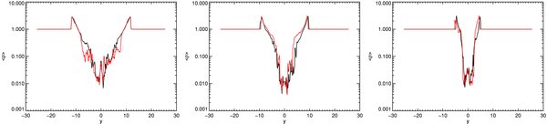
Figure 26. One-dimensional profiles of quantities transverse to the jet axis, ρavg(x) = 0.5[ρ(x, y = 0, z) + ρ(x, y, z = 0)] at x = 12.8 (left panel), x = 25.6 (center panel), and x = 38.4 (right panel) for the HLLC (black lines) and HLLD (red lines) solvers calculated at t = 100.
Download figure:
Standard image High-resolution image
Figure 27. Same as Figure 26, but for βavg(x) = 2(Pg)avg(x)/|b|2avg(x).
Download figure:
Standard image High-resolution imageAn alternative measure of the effective resolution of these jet simulations is through the normalized gradient of a quantity, |∇Q|/Q. Mignone et al. (2009) compared the evolution of the gradients of the poloidal magnetic field |∇B2p|/B2p for axisymmetric simulations computed at a range of resolutions for the HLLE and HLLD solvers, finding a factor of two increase in the effective resolution by this measure. Figure 28 shows the volume average of the normalized gradient of Q, 〈|∇Q|/Q〉 for Q = ρ, Γ, |b|2 at t = 100 for each of the simulations described above. According to the measures 〈|∇ρ|/ρ〉 and 〈|∇Γ|/Γ〉, simulations computed using the HLLC and HLLD solvers have the same effective resolution. The measure 〈|∇|b|2|/|b|2〉 indicates that the effective resolution of the HLLD solver is a factor of 3–4 greater than that of the HLLC solver; we also find that 〈|∇|b|2|/|b|2〉 for the HLLC solver at the highest resolution is still smaller than 〈|∇|b|2|/|b|2〉 for the HLLD solver at the lowest resolution. Examination of the profile of 〈|∂y|b|2 + ∂z|b|2|/|b|2〉 along the jet axis (where the averaging is now performed on surfaces of constant x) suggests that 〈|∇|b|2|/|b|2〉 is enhanced in the HLLD simulations throughout the jet, rather than being concentrated in one region, i.e., in the HLLD simulations, the entirety of the jet cocoon is filled with magnetic fields that are both stronger (by up to an order of magnitude) and possess steeper gradients (by up to a factor of four) than simulations conducted with the HLLC solver at the same resolution, further demonstrating the importance of the rotational discontinuity.

Figure 28. Volume-averaged normalized gradient, 〈|∇Q|/Q〉, for density, ρ (crosses), Lorentz factor, Γ (triangles), and magnetic field strength, |b|2 (squares), for simulations computed with the HLLC (blue lines) and HLLD (red lines) Riemann solvers for simulations with 5, 10, and 20 zones per jet radius.
Download figure:
Standard image High-resolution imageOverall, these simulations demonstrate that, for the second-order integration scheme presented here, use of more complex Riemann solvers for three-dimensional evolutions of relativistic jets is essential in order to correctly capture the dynamics of the magnetic field. However, we once again caution that without explicit dissipation and physical perturbations, the solutions shown here are not converged. Therefore, as in the previous section, these simulations serve as a qualitative demonstration of the importance of utilizing advanced Riemann solvers in studying multi-dimensional nonlinear flows.
6. SUMMARY
We have described a new, second-order accurate Godunov scheme for RMHD. This scheme is distinguished from previous work in two important respects. First, we utilize the staggered, face-centered field version of the CT algorithm with the method of Gardiner & Stone (2005, 2008) to compute the electric fields at cell edges, which keeps the cell-centered, volume-averaged discretization of the divergence to zero to machine precision. Second, we make use of a dimensionally unsplit integrator (Stone & Gardiner 2009) which preserves the conservative form of the RMHD equations without the need for characteristic decomposition of the equations of motion in the primitive variables. Because of the tight coupling between the conserved variables in RMHD, maintaining both the divergence condition and the conservative form of the equations offers clear advantages over either divergence cleaning methods (Anninos et al. 2005; Mignone et al. 2010) or dimensionally split methods (Powell et al. 1999).
We documented four additional parts of the algorithm that we have found important: a scheme for computing the primitive variables from conserved quantities, which we base on the 1 DW scheme described by Noble et al. (2006), as modified by Mignone et al. (2007); the method for calculating the wave speeds in RMHD, which amounts to finding the roots of a quartic polynomial; a variety of approximate Riemann solvers used to compute fluxes in RMHD; and a hierarchy of correction steps designed to correct errors corresponding to unphysical primitive variables. We have made the resulting numerical scheme publicly available as part of the Athena code (Stone et al. 2008).
We presented a variety of multi-dimensional numerical tests which build on those previously available in the literature for both relativistic and Newtonian MHD. The solutions to these tests are designed to highlight important properties of the numerical method, such as its ability to hold symmetry, or to test that the solenoidal constraint is preserved on the correct numerical stencil. Of these tests, we have found the large amplitude circularly polarized Alfvén wave test of Del Zanna et al. (2007) and the field-loop advection test to be particularly revealing. The former of these revealed failures in the HLLC Riemann solver due to Mignone & Bodo (2006) due to a flux singularity that exists for multi-dimensional MHD problems; the latter test probes both the codes ability to maintain the solenoidal constraint on the correct numerical stencil (Gardiner & Stone 2005, 2008) and the ability of the primitive variable inversion scheme to maintain a uniform, non-zero velocity field when fluid momentum, energy, density, and magnetic field are advected obliquely to the grid.
We demonstrated that the integration scheme is able to evolve strong blast waves in strongly magnetized media via a modified version of the relativistic blast wave originally due to Komissarov (1999a). In this modification, the blast wave achieves a terminal Lorentz factor of Γ = 1.8, while allowing the evolution of magnetic fields with strengths correspond to β = 10−8 in the ambient medium. Comparing results between blast waves of different strengths in media with different degrees of magnetization using both relativistic and non-relativistic physics led us to the conclusion that problems in previously reported blast wave tests arise not due to imbalances in the energy equation (see, e.g., Del Zanna et al. 2007), but due to errors in the primitive variable inversion scheme.
We applied the integration scheme to two interesting problems in computational relativistic astrophysics: the development of the KHI and the propagation of a relativistic magnetized jet. Simulations of the KHI were computed in both two and three dimensions using a variety of approximate Riemann solvers. The development and the turbulence arising from the instability was found to be strongly affected by the choice of Riemann solver. The most diffusive solver, the HLLE approximate Riemann solver, produced converged solutions at the end of the linear growth phase of the instability that lacked secondary vortices clearly present at the same time in solutions computed at a factor 322 lower in resolution with the HLLC and HLLD approximate Riemann solvers, which differ from the HLLE solver by the presence of contact (HLLC/D) and rotational discontinuities (HLLD). In three dimensions, these lacks strongly affected the structure of the nonlinear turbulence that arose from the instability. Since the scheme is stable and the HLLE solver is consistent, this result suggests that solutions computed using the HLLE solver converge to a different weak solution to the conservation law than those computed using the HLLC and HLLD solvers (LeVeque 2002).
The final problem that we considered was that of the evolution of a relativistic, magnetized jet, the highest resolution simulations of which were computed using SMR. These simulations were used to probe the impact of rotational discontinuities on the structure of the magnetic field within the jet. Simulations computed with Riemann solvers that contained these discontinuities (HLLD) exhibited magnetic fields within the jet cocoon that were an order of magnitude stronger and contained a factor of 3–4 more structure than simulation computed with Riemann solvers that did not (HLLE). Furthermore, simulations using the former exhibited strongly magnetized sheath that surrounded jet core, which was absent in simulations using the latter. The large-scale dynamics of astrophysical jets are thought to be intimately tied to the mechanisms through which magnetic fields close to the launch sites are dissipated and as such our results demonstrate the importance of utilizing more accurate Riemann solvers for such studies.
The algorithms described here are but a first step in extending the Athena code to RMHD. Future algorithmic projects will include extending the integrator described here to generalized curvilinear coordinates (i.e., GRMHD), extending the primitive variable inversion scheme to other equations of state (e.g., the Synge gas Mignone & McKinney 2007), and possibly an extension of the "CTU+CT" integrator of Gardiner & Stone (2005, 2008) to relativistic fluids, utilizing the work of Antón et al. (2010). Finally, we will apply the algorithms described here to a full investigation of the relativistic KHI and current-driven instabilities in relativistic magnetized jets in future work.
This work was supported by NASA under grant NNX09AG02G from the Astrophysics Theory and Fundamental Physics program, under NNX09AB90G from the Origins of Solar Systems Program, and by the NSF under grants AST-0807471 and AST-0908269. The authors acknowledge the Texas Advanced Computing Center (TACC) at The University of Texas at Austin, and the Princeton Institute of Computational Science and Engineering, for providing HPC and visualization resources. We thank Phil Armitage, Mitch Begelman, Alexander Tchekhovskoy, Jon McKinney, and Andrea Mignone for useful discussions and advice. Finally, we thank Phil Armitage, Charles Gammie, Alexander Tchekhovskoy, and an anonymous referee for careful reading of the manuscript and making several suggestions that greatly improved earlier versions of this work.
Footnotes
- 3
- 4
Note that this is not to say that we would be unable to recover the case Vz = 0 when ; this is guaranteed by the equation defining Vi in terms of these quantities.
