

Abstract
Quantum error correction (QEC) and fault-tolerant quantum computation represent one of the most vital theoretical aspects of quantum information processing. It was well known from the early developments of this exciting field that the fragility of coherent quantum systems would be a catastrophic obstacle to the development of large-scale quantum computers. The introduction of quantum error correction in 1995 showed that active techniques could be employed to mitigate this fatal problem. However, quantum error correction and fault-tolerant computation is now a much larger field and many new codes, techniques, and methodologies have been developed to implement error correction for large-scale quantum algorithms. In response, we have attempted to summarize the basic aspects of quantum error correction and fault-tolerance, not as a detailed guide, but rather as a basic introduction. The development in this area has been so pronounced that many in the field of quantum information, specifically researchers who are new to quantum information or people focused on the many other important issues in quantum computation, have found it difficult to keep up with the general formalisms and methodologies employed in this area. Rather than introducing these concepts from a rigorous mathematical and computer science framework, we instead examine error correction and fault-tolerance largely through detailed examples, which are more relevant to experimentalists today and in the near future.
Export citation and abstract BibTeX RIS
1. Introduction
The micro-computer revolution of the late 20th Century has arguably had a greater impact on the world than any other technological revolution in history. The advent of transistors, integrated circuits, and the modern microprocessor has spawned literally hundreds of devices, from pocket calculators to the iPod, all now integrated through an extensive worldwide communications system. However, as we enter the 21st Century, ever increasing computational power is driving us quickly to the realm where quantum physics dominates. The component size of individual transistors on modern microprocessors is becoming so small that quantum effects will soon begin to dominate. Unfortunately, quantum mechanical behaviour will tend to result in unpredictable and unwanted operation in classical microprocessor designs. We therefore have two choices: keep trying to suppress quantum effects in classically fabricated electronics, or move to the field of quantum information processing (QIP) where we exploit them. This leads to a paradigm shift in the way we view and process information and has commanded considerable interest from physicists, engineers, computer scientists and mathematicians. The counter-intuitive and strange rules of quantum physics offer enormous possibilities for information processing and the development of a large-scale quantum computer is the holy grail for many researchers worldwide.
While the advent of Shor's algorithm [Sho97] certainly spawned great interest in QIP, demonstrating that quantum algorithms could be far more efficient than those used in classical computing, there was a great deal of debate surrounding the practicality of building a large scale, controllable, quantum system. It was well known even before the introduction of quantum information that coherent quantum states were extremely fragile and many believed that to maintain large, multi-qubit, coherent quantum states for a long enough time to complete any quantum algorithm was unrealistic [Unr95]. Additionally, classical error correction techniques are intrinsically based on a digital framework, unlike quantum computing where the readout of qubits is digital but actual manipulations are analogue. Therefore, how can we adapt the vast knowledge gained from classical coding theory to the quantum regime?
Starting in 1995, several papers appeared, in rapid succession, proposing codes which were appropriate to perform error correction on quantum data [Sho95, Ste96a, CS96, LMPZ96, BSW96]. This was a key theoretical development needed to convince the general community that quantum computation was indeed a possibility. Since this initial introduction, the progress in this field has been extensive.
Initial research on error correction focused heavily on developing quantum codes [Ste96c, Ste96b, Got96, PVK97, KL97, Kni96], introducing a more rigorous theoretical framework for the structure, properties and operation of QEC [BSW96, KL00, CRSS98, Got97, CG97, KLV00]. Addi tionally, the introduction of concepts such as fault-tolerant quantum computation [Sho96, DS96, Got98, KLZ98, Got00] led directly to the threshold theorem for concatenated QEC [KLZ96, ABO97]. In more recent years, QEC protocols have been developed for various systems, such as continuous variables [LS98, Bra98, vL08, ATK+09], ion-traps and other systems containing motional degrees of freedom [ST00], adiabatic computation [JFS06] and globally controlled quantum computers [BBK03]. Work also continues on not only developing better (and in some ways, more technologically useful) protocols such as subsystem codes [KLP05, KLPL06, Bac06] and topological codes [Kit97, DKLP02, BMD06, BMD07b, BMD07a, RHG07, FSG09]. Advanced techniques to analyse fault-tolerant thresholds [AGP08, PR12, BMD08, BAO+12] have also been developed to implement error correction in a fault-tolerant manner with concatenated codes [Ste97a, Ste02, DA07, Kni05] and topological codes [BMD07b, KBAMD10, Bom11].
Along with QEC, other methods of protecting quantum information were also developed. These other techniques would technically be placed in a separate category of error suppression rather than error correction. The distinction between error suppression and error correction is also known as passive and active QEC, the latter terminology being much more prevalent in the theoretical community. The most well known techniques of error suppression are protocols such as decoherence free subspaces (DFS) [PSE96, DG97, LCW98, DG98b, ZR97b, ZR97a, DG98a, LW03]. DFS protocols are passive, encoding information in a subspace which is invariant under the dynamics that generate errors. Active methods for error suppression include applying repeated rotations to qubits such that these rotations, combined with the natural dynamics that induce errors, partially cancel. These methods were initially referred to as Bang-Bang control [VL98, VT99, Zan99] and developed primarily for NMR systems. In recent years these techniques have been further generalized and optimized for use in essentially all QIP systems [VKL99, FLP04, VK03, VK05, KL05, Uhr07]. These more advanced techniques are now routinely categorized as dynamical decoupling protocols. As with QEC, this field is vast, incorporating well established ideas from quantum control to create specially designed control sequences to suppress errors before more resource intensive encoding is applied.
This review deals exclusively with the concepts of QEC and fault-tolerant quantum computation. Many papers have reviewed error correction and fault-tolerance [Got97, NC00, Got02, KLA+02, Ste01, Got09], however to cater for a large audience, we attempt to describe QEC and fault-tolerance in a more basic manner, largely through examples. Instead of providing a more rigorous review of error correction, we instead focus on more practical issues involved when working with these ideas. For those who have recently begun investigating QIP or those who are focused on other important theoretical and/or experimental aspects related to quantum computing, searching through this enormous collection of work is daunting especially if a basic working knowledge of QEC is all that is required. This review of the basic aspects of QEC and fault-tolerance is designed to allow those with little knowledge of the field to quickly become accustomed to the various techniques and tricks that are commonly used. The examples in this review are selected due to their relative simplicity. For individuals seriously interested in examining new ideas for QEC and fault-tolerant computation we strongly advise that the references cited throughout are consulted.
We begin the discussion in section 2 where we describe some preliminary concepts on the required properties of any quantum error correcting protocol. In section 3 we review some basic noise models in the context of how they influence quantum algorithms. Section 4 introduces quantum error correction through the traditional example of the 3-qubit code, illustrating the circuits used for encoding and correction and why the principle of redundant encoding suppresses the failure of encoded qubits. Sections 5 and 6 introduce the first examples of complete quantum codes, Shor's 9-qubit code and a 4-qubit error detection code. Sections 7 and 8 introduce the stabilizer formalism, demonstrating how QEC circuits are synthesized once the structure of the code is known. In section 9 we briefly return to noise models and relate the abstract analysis of QEC, where errors are assumed to be discrete and probabilistic, to some of the physical mechanisms which can cause errors. Sections 10 and 11 introduce the concept of fault-tolerant error correction, the threshold theorem and how logical gate operations can be applied directly to encoded data. We then move onto circuit synthesis in section 12, presenting a fault-tolerant circuit design for state preparation using the 7-qubit Steane code as a representative example. Finally, in section 14, we review specific codes for qubit loss and examine two more modern techniques for error correction. We briefly examine quantum subsystem codes [KLP05, KLPL06, Bac06] and topological surface codes [DKLP02, FSG09] due to both their theoretical elegance and their increasing relevance in quantum architecture designs [IFI+02, DFS+09, SJ09, MLFY10].
2. Preliminaries
Before discussing quantum errors and how they can be corrected, we first introduce the basics of qubits and quantum gates. We assume a basic working knowledge with quantum information [EJ96, NC00] and this brief discussion is used simply to define our notation for the remainder of this review.
2.1. Basic structure of the qubit
The fundamental unit of quantum information is the qubit. Unlike the classical bit, the qubit can exist in coherent superpositions of its two states, denoted as |0〉 and |1〉. These basis states can be, for example, photonic polarization, atomic spin states, electronic states of an ion or charge states of superconducting systems. An arbitrary state of an individual qubit, |φ〉, can be expressed as

where |0〉 and |1〉 are the two orthonormal basis states of the qubit and |α|2 + |β|2 = 1. Quantum gate operations are represented by unitary operations acting on the Hilbert space of a collection of qubits. Unlike classical information processing, conservation of probability for quantum states requires that all operations be reversible and hence unitary.
When describing a quantum gate on an individual qubit, any dynamical operation, G, is a member of the unitary group U(2), which consists of all 2 × 2 matrices where G† = G−1. Up to a global (and unphysical) phase factor, any single qubit operation can be expressed as a linear combination of the generators of SU(2) as,

where

are the Pauli matrices, σI is the 2 × 2 identity matrix, cI is a real number, and (cx, cy, cz) are complex numbers satisfying,

Here ℜ and ℑ are the real and imaginary components, respectively.
2.2. Some general requirements of quantum error correction
Although the field of QEC is largely based on classical coding theory, there are several issues that need to be considered when transferring classical error correction techniques to the quantum regime.
First, coding based on data-copying, which is extensively used in classical error correction, cannot be used due to the no-cloning theorem of quantum mechanics [WZ82]. This result implies that there exists no transformation resulting in the following mapping,

i.e. it is impossible to perfectly copy an unknown quantum state. This means that quantum data cannot be protected from errors by simply making multiple copies. Secondly, direct measurement cannot be used to effectively protect against errors, since this will act to destroy any quantum superposition that is being used for computation. Error correction protocols must therefore be employed, which can detect and correct errors without determining any information regarding the qubit state. Unlike classical information, qubits are susceptible to both traditional bit errors |0〉 ↔ |1〉, and also phase errors |0〉 ↔ |0〉, |1〉 ↔ −|1〉. Hence any error correction procedure needs to be able to simultaneously correct for both. Finally, errors in quantum information are intrinsically continuous (i.e. qubits do not experience full bit or phase flips but rather an angular shift of the qubit state by any angle). This issue will be discussed in more depth in section 9.
At its most basic level, QEC utilizes the idea of redundant encoding. This is where the total size of the Hilbert space is expanded beyond what is needed to store a single qubit of information. This way, errors on individual qubits are mapped to a large set of mutually orthogonal subspaces, the size of which is determined by the number of qubits utilized in the code. Finally, the error correction protocol cannot allow us to gain information regarding the coefficients, α and β of the encoded state, as doing so would collapse the system.
3. Quantum errors: cause and effect
Before we begin discussing the details of QEC, we first examine some of the common sources of errors in QIP and contextualize what they imply for computation. We will consider several important sources of errors and how they influence two trivial, single qubit quantum algorithms.
The first algorithm is a computation consisting of a single qubit, initialized in the |0〉 state undergoing N identity operations. If this algorithm is performed perfectly the final state is,

where I ≡ σI is the identity gate. Measurement of the qubit in the |0〉, |1〉 basis will consequently yield the result 0 with a probability of unity.
The second illustration is an algorithm of three gates,

This algorithm will ideally yield a result |0〉 with probability of 1 when measured in the |0〉, |1〉 basis. This algorithm implements two H ≡ Hadamard operations separated by a wait stage, represented by the Identity gate.
We examine, independently, several common sources of error from the effect they have on these two quantum algorithms. Hopefully, this introductory section will show that while quantum errors are complicated physical effects, in QIP the relevant measure is the theoretical success probability of a given quantum algorithm.
Errors that exist on any quantum system are highly dependent on the specific physical mechanisms that govern the system. The situations that follow are only basic illustrative examples which can often arise in discussions related to errors and QEC. It is important to stress that the types of errors and the way in which they are analysed need to be considered in the context of the physical system under consideration.
3.1. Coherent quantum errors: gates which are incorrectly applied
The first possible source of error is coherent, systematic control errors. This type of error is typically associated with incorrect knowledge of the system dynamics. Namely, otherwise perfect control assuming a system governed by a Hamiltonian H' when the actual system dynamics is governed by H. As qubit systems must be characterized prior to being used [PCZ97, CSG+05], finite experimental resolution with these processes will lead to coherent control errors. As these errors are coherent inaccuracies applied to the qubit, they can be mitigated using coherent techniques such as composite pulse sequences [LF79, Lev86, BHC04, Jon09]. Other control errors (e.g. arising from fluctuations in control fields) are not coherent processes and are dealt with in a similar way to environmental coupling described further on.
As this source of error is coherent and systematic it causes one to apply the same, undesired gate operation and can be analysed without moving to the density matrix formalism. With respect to the first of our algorithms, we are able to model this in several different ways. To keep things simple, we assume that incorrect characterization of the control dynamics leads to a gate which is not σI, but instead introduces a small rotation around the X-axis of the Bloch sphere. This results in the state,

We now measure the system in the |0〉, |1〉 basis. Due to these errors, the probability of measuring the system in the |0〉 or |1〉 state is,

Hence, the probability of error in this trivial quantum algorithm is given by perror ≈ (N )2, which will be small given that N ≪ 1. The systematic error in this system is quadratic in both the small systematic over rotation and the total number of applied identity operations. This is expected as this rotational error always acts in the same direction every time it is applied.
3.2. Environmental decoherence
Environmental decoherence is another important source of errors in quantum systems. We will take a simple decoherence model and examine how our second algorithm behaves. Later in section 9 we will illustrate a more complicated decoherence model that arises from standard mechanisms.
Consider a very simple environment, which is another two level quantum system. This environment has two basis states, |e0〉 and |e1〉, that satisfy the completeness relations,

We will also assume that the environment couples to the qubit in a specific way. When the qubit is in the |1〉 state, the coupling flips the environmental state, while if the qubit is in the |0〉 state nothing happens to the environment. Finally, this model assumes the system/environment interaction only occurs during the wait stage of the algorithm (while the Identity gate is being applied). As with the first algorithm we should measure the state |0〉 with probability one. The reason for utilizing the second of our algorithms in this example is that this specific decoherence model acts to reduce coherence between the |0〉 and |1〉 states. Therefore, we require a coherent superposition to observe any effect from the environmental coupling. We assume the environment is initialized in the state, |E〉 = |e0〉, and then coupled to the system,

As we are considering environmental decoherence, pure states will be transformed into classical mixtures, hence we now move into the density matrix representation for the state HIH|0〉|E〉,

As we have no access to the environmental degrees of freedom, we trace over this part of the system, giving,

Measurement of the system will consequently return |0〉 50% of the time and |1〉 50% of the time. This final state is a complete mixture of the two qubit states and is consequently a classical system. The coupling to the environment removed all the coherences between the |0〉 and |1〉 states and the second Hadamard transform, intended to rotate
 , has no effect on the qubit state.
As we assumed that the system/environment coupling during the wait stage causes the environmental degree of freedom to 'flip' (when the qubit is in the |1〉 state) this decoherence model implicitly incorporates a temporal effect. The temporal interval of the identity gate in the above algorithm is long enough to enact the controlled-flip operation. If we assumed a controlled rotation that was not a full flip on the environment, the final mixture would not be 50/50. Instead there would be a residual coherence between the qubit states and an increased probability of our algorithm returning a |0〉. Section 9 revisits the decoherence model and illustrates how time-dependence is explicitly incorporated.
3.3. Simple models of loss, leakage, measurement and initialization
Other sources of error such as qubit initialization, measurement errors, qubit loss and qubit leakage can be modelled in a very similar manner. As with coherent control errors and environmental decoherence, the specifics of other error channels can be modelled in a coherent or incoherent manner, depending on the physical mechanisms. The examples shown below are commonplace within QEC analysis and adequately apply to a large number of systems.
Measurement errors can be modelled in the same way as environmental decoherence, acting incoherently on the system. Measurement errors can be described in two slightly different ways. The first is to use the following positive operator value measures (POVMs),

where pM is the probability of measurement error. These are not measurement projectors as
 and
and
 . The second method is to apply the following mapping to the qubit,

followed by a perfect measurement in the (|0〉, |1〉) basis. These two models give exactly the same probabilities for each outcome. Defining A0 = |0〉〈0| and A1 = |1〉〈1| as the measurement projectors onto the (|0〉, |1〉) basis we find


Hence, either method will result in the same probabilities for a given value of pM. The difference between these two models is the state the measured qubit is projected to.
When using the POVMs in equation (14), the collapsed state of the qubit is given by

where

Therefore the resulting state, after measurement, will not be initialized in a known state. If the second model is used, then the system is initialized to either |0〉 or |1〉 depending on which projector is used. To see this explicitly, consider the state,

Using both models, the probability of measuring |0〉 is 1/2 (as the above state is invariant under a bit-flip error). If the POVM model is used (using the F0 and M0 operators), the state after measurement is,

The collapsed state, after measurement, is a superposition of |0〉 and |1〉, with amplitudes related to pm. If we use the second model (using the projector A0), the state after measurement is simply |0〉. As measurement is generally followed by either discarding the qubit or reinitializing it in a known state, both models can generally be used interchangeably with no adverse consequences.
Qubit loss is modelled in a slightly different manner. When a qubit is lost, it is effectively removed from the system. This channel can be modelled by simply tracing out the lost qubit, Tri(ρ), where i is the index of the lost qubit. This reduces the dimensionality of the qubit space by a factor of two.
The loss of the physical object means that it cannot be directly measured or coupled to any other ancillary system. Even though this model of qubit loss (with regards to the information stored on the qubit) is equivalent to incoherent processes such as environmental coupling, correcting this type of error requires additional machinery on top of standard QEC protocols. Standard correction protocols can protect against the loss of information on a qubit, provided that the physical object still exists in the computer. Therefore, an initial non-demolition detection must be employed (which determines if the qubit is actually present without performing a projective measurement on the computational state) before standard correction can correct the error. Provided that these non-demolition protocols are employed, loss actually becomes a preferred channel in error correction. If a loss event is detected and the quit is replaced, this heralds the qubit experiencing the error. This additional information can be used within error correction protocols to increase performance.
Initialization of the qubit can be modelled either using a coherent systematic or incoherent process. If an incoherent model is employed, initialization can be modelled in essentially the same way as imperfect measurement. If we have a probability pI of initialization error (where pI encapsulates the internal mechanisms that introduce errors) and we initialize the qubit in the |0〉 state, the initial state of the system is given by the mixture,

In contrast, we could consider an initialization model which is achieved via a coherent unitary operation where the target is the desired initial state. In this case, the initial state is pure, but contains a non-zero amplitude of the undesired target, for example,

where |α|2 + |β|2 = 1 and |β|2 ≪ 1. The interpretation of these two types of initialization models is identical to the coherent and incoherent models presented. Again, the effect of these types of errors relates to the probabilities of measuring the system in an erred state.
One final type of error that we can briefly mention is qubit leakage. Qubit leakage manifests due to the fact that most systems utilized for qubits do not consist of just two levels. For example, figure 1 (from [Ste97b]) illustrates the energy level structure for a 43Ca+ ion utilized for ion trap quantum computing. The qubits in this system are defined with two electronic states, however the system itself contains many more levels (including some which are used for qubit readout and initialization). As with systematic errors, leakage can occur when improper control is applied to such a system. In the case of ion-traps, qubit transitions are performed by focusing finely tuned lasers resonant on the relevant transitions. If the laser frequency fluctuates or additional levels are not sufficiently detuned from the qubit resonance, the following transformation could occur,

where the state |2〉 is a third level, which is now populated due to improper control. The actual effect of this type of error can manifest in several different ways. As quantum circuits and algorithms are fundamentally designed assuming the computational array is of a 2-level system, the transformation shown in equation (24) (which in this case is operating over a 3-level space) will naturally induce unwanted dynamics. Another important implication of applying non-qubit operations is how these levels interact with the environment and hence how decoherence affects the system. For example, in the above case, the unwanted level, |2〉, may be extremely short lived leading to an emission of a photon and the system relaxing back to the ground state. For these reasons, leakage is one of the most problematic error channels to correct using QEC. In general, leakage induced errors need to be corrected in a similar manner to loss, which can also be thought of as a leakage process into a vacuum state. Non-demolition techniques are first required to determine if the system is still confined to the qubit subspace [Pre98, GBP97, VWW05] after which standard correction protocols can be utilized. As with qubit loss, if these additional protocols are employed, leakage errors are heralded and the performance of the resulting error correction will increase.

Figure 1. (From [Ste97b]) Energy level structure for the 43Ca+ investigated by the Oxford ion-trapping group. The structure of this ion is clearly not a 2-level quantum system. Hence leakage into non-qubit states is an important factor to consider.
Download figure:
Standard image High-resolution imageAnother well known method is to use a complicated pulse sequence which acts to re-focus an improperly confined operation back to the qubit subspace [WBL02, BLWZ05]. This can be advantageous as it does not require additional qubit resources.
Leakage effects arise from multiple sources, and the best method for correction is often heavily dependent on the error mechanisms. One example is when internal fluctuations in the system change otherwise perfect qubit dynamics. Unfortunately this leakage source generally cannot be predicted and/or characterized and so dedicated leakage protection will need to be employed. A second source is imprecise fabrication of an otherwise perfect qubit system. This source of leakage can, in principal, be engineered away, thereby eliminating the need for specialized leakage correction. In the context of mass manufacturing of qubit systems, leakage would ideally be quantified immediately after the fabrication of a device [DSO+07] to eliminate these systematic leakage errors. If a particular system was found to be improperly confined to the qubit subspace, it would simply be discarded. Employing characterization at this stage could potentially eliminate the need to implement a large amount of leakage protection in the computer, shortening gate times and ultimately reducing error rates in the computer.
In this section we have presented a very basic set of examples to explain some of the ideas of quantum errors and how they affect the success of a quantum algorithm. Section 9 will return to a more realistic set of error models. For those interested in a more complete treatment of quantum errors we encourage readers to refer to [Got97, NC00, Got02, KLA+02, Ste01, Got09].
4. The 3-qubit code: a good starting point for quantum error correction
The 3-qubit bit-flip code is traditionally used as a basic introduction to the concept of quantum error correction. It should be emphasized that the 3-qubit code does not represent a full quantum code. This is due to the fact that the code cannot simultaneously correct for both bit and phase flips (section 9). This code is a repetition code extended by Shor [Sho95] to construct the 9-qubit quantum code, demonstrating that QEC was possible.
The 3-qubit code encodes a single logical qubit into three physical qubits with the property that it can correct for a single, σx, bit-flip error. The two logical basis states |0〉L and |1〉L are defined as

such that an arbitrary single qubit state |ψ〉 = α|0〉 + β|1〉 is mapped to,

Figure 2 illustrates the quantum circuit required to encode a single logical qubit via the initialization of two ancilla qubits and two CNOT gates. The reason that this code is able to correct for a single bit-flip error is the binary distance between the two codeword states. Notice that three individual bit flips are required to take |0〉L ↔ |1〉L, hence if we assume |ψ〉 = |0〉L, a single bit flip on any qubit leaves the final state closer to |0〉L than |1〉L. The distance between two codeword states, d, defines the number of errors that can be corrected, t, as t = ⌊(d − 1)/2⌋. In this case, d = 3, hence t = 1.

Figure 2. Quantum circuit to prepare the |0〉L state for the 3-qubit code where an arbitrary single qubit state, |ψ〉 is coupled to two freshly initialized ancilla qubits via CNOT gates to prepare |ψ〉L.
Download figure:
Standard image High-resolution imageHow are we able to correct errors using this code without directly measuring or obtaining information about the logical state? Two additional ancilla qubits are introduced, which are used to extract syndrome information (information regarding possible errors) from the data block without discriminating the exact state of any qubit. The encoding and correction circuit is illustrated in figure 3. Correction proceeds by introducing two ancilla qubits and performing a sequence of CNOT gates, which checks the parity of the three qubit data block. For the sake of simplicity we assume that all gate operations are perfect and the only place where the qubits are susceptible to error is the region between encoding and correction (as illustrated in figure 3). We will return to this issue in section 10 when we discuss fault-tolerance. We also assume that at most a single, complete bit-flip error occurs on one of the three data qubits. Table 1 summarizes the state of the whole system, for each possible error, just prior to measurement.

Figure 3. Circuit required to encode and correct for a single σx-error. We assume that after encoding a single bit-flip occurs on one of the three qubits (or no error occurs). Two initialized ancilla are then coupled to the data block which only checks the parity between qubits. These ancilla are then measured, with the measurement result indicating where (or if) an error has occurred, without directly measuring any of the data qubits. Using this syndrome information, the error can be corrected with a classically controlled σx gate.
Download figure:
Standard image High-resolution imageTable 1. Final state of the five qubit system prior to the syndrome measurement for no error or a single X error on one of the qubits. The last two qubits represent the state of the ancilla. Note that each possible error will result in a unique measurement result (syndrome) of the ancilla qubits. This allows for a σx correction gate to be applied to the data block which is classically controlled from the syndrome result.
| Error location | Final state, |data〉|ancilla〉 |
|---|---|
| No error | α|000〉|00〉 + β|111〉|00〉 |
| Qubit 1 | α|100〉|11〉 + β|011〉|11〉 |
| Qubit 2 | α|010〉|10〉 + β|101〉|10〉 |
| Qubit 3 | α|001〉|01〉 + β|110〉|01〉 |
For each possible situation, either no error or a single bit-flip error, the ancilla qubits are flipped to a unique state based on the parity of the data block. These qubits are then measured to obtain the classical syndrome result. The result of the measurement will then dictate if a correction gate needs to be applied. This is illustrated in table 2.
Table 2. Ancilla measurements for a single σx error with the 3-qubit code. Each of the four possible results correspond to either no error or a bit flip on one of the three qubits.
| Ancilla measurement | Collapsed state | Consequence |
|---|---|---|
| 00 | α|000〉 + β|111〉 | No error |
| 01 | α|001〉 + β|110〉 | σx on qubit 3 |
| 10 | α|010〉 + β|101〉 | σx on qubit 2 |
| 11 | α|100〉 + β|011〉 | σx on qubit 1 |
Provided that only a single error has occurred, the data block is restored. At no point during correction do we gain any information regarding the coefficients α and β, hence superpositions of the computational state will remain intact during correction.
This code will only work if a maximum of one error occurs. The 3-qubit code is a d = 3 code, hence if t > 1, then the resulting state becomes 'closer' to the wrong logical state. This can be seen in table 3 when tracking multiple errors through the correction circuit. In each case, we assume that the total number of errors is >d/2, therefore our correction takes us to the wrong logical state. In every case where t > 1 our mis-correction induces a logical bit flip, causing the code to fail.
Table 3. Ambiguity of syndrome results when multiple errors occur.
| Error location | Final state, |data〉|ancilla〉 | Assumed error |
|---|---|---|
| Qubit 1 and 2 | α|110〉|01〉 + β|001〉|01〉 | σx on qubit 3 |
| Qubit 2 and 3 | α|011〉|11〉 + β|100〉|11〉 | σx on qubit 1 |
| Qubit 1 and 3 | α|101〉|10〉 + β|010〉|10〉 | σx on qubit 2 |
| Qubit 1, 2 and 3 | α|111〉|00〉 + β|000〉|00〉 | No error |
To be absolutely clear on how QEC acts to restore the system and protect against errors let us now consider a different and slightly more physically realistic example. We will assume that the errors acting on the qubits are coherent rotations of the form U = exp(iσx) on each qubit, with ≪ 1. We choose coherent rotations so that we can remain in the state vector representation. This is not a necessary requirement, however more general incoherent mappings would require us to move to density matrices.
We assume that each qubit experiences the same error, hence the error operator acting on the state is

where

Now let us examine the transformation that occurs when we run the error correction circuit in figure 3. This is represented via the unitary transformation, UQEC, over both the data and ancilla qubits,

Once again, the ancilla block is measured and the appropriate correction operator is applied, yielding the results (up to renormalization) shown in table 4. In each case, after correction (based on the syndrome result), we are left with approximately the same state, a superposition of a 'clean state' with the logically flipped state, σxσxσx|ψ〉. Let us now examine in detail the amplitudes now associated with each term in these states. If we consider the unitary U acting on a single, unencoded qubit, the rotation takes the state |ψ〉 to,

Table 4. Resulting logical state after a round of error correction with the 3-qubit code.
| Ancilla measurement | Collapsed state (with correction) |
|---|---|
| 00 | c0|ψ〉L + c3σxσxσx|ψ〉L |
| 01 | c1|ψ〉L + c2σxσxσx|ψ〉L |
| 10 | c1|ψ〉L + c2σxσxσx|ψ〉L |
| 11 | c1|ψ〉L + c2σxσxσx|ψ〉L |
Consequently, the fidelity of the single qubit state is,

In contrast, the worst case fidelity3 of the encoded qubit state after a cycle of error correction is,

with probability 1 − 32 + O(4) and

with probability 32 + O(4). This is the general idea of how QEC suppresses errors at the logical level. During a round of error correction, if no error is detected, the error on the resulting state is suppressed from O(2) to O(6). If a single error is detected, the fidelity of the resulting state remains the same. As the 3-qubit code is a single error correcting code, if one error has already been corrected then the failure rate of the logical qubit is conditional on experiencing one further error (which will be proportional to 2). As ≪ 1 the majority of correction cycles will detect no error and the fidelity of the resulting encoded state is higher than when unencoded.
It should be stressed that no error correction scheme will, in general, fully restore a corrupted state to the original logical state. The resulting state will generally contain a superposition or a mixture of a clean state and a logically erred state depending on whether the error process is coherent or incoherent. The point is that the fidelity of the corrupted states, at the logical level, is greater than the corresponding fidelity for unencoded qubits. Consequently the probability of measuring the correct result at the end of a specific algorithm increases when the system is encoded. The example shown here is somewhat unphysical, i.e. it assumes perfect gate operations, errors that only consist of σx-rotations at a specific point in the circuit. In the coming sections we will introduce the concepts necessary when relaxing these assumptions.
5. The 9-qubit code: the first full quantum code
The 9-qubit error correcting code was first developed by Shor [Sho95] in 1995 and is based largely on the 3-qubit repetition code. The Shor code is a degenerate4 single error correcting code, able to correct a logical qubit from one bit-flip, one phase-flip or one of each, on any of the nine physical qubits. This code is therefore sufficient to correct for an arbitrary single qubit error (section 9). The two basis states for the code are

and the circuit to perform the encoding is shown in figure 4. Correction for X errors, for each block of three qubits encoded to
 is identical to the 3-qubit code shown earlier. By performing the correction circuit shown in figure 3 for each block of three qubits, single σx ≡ X errors can be detected and corrected. Phase errors (σz ≡ Z) are corrected by examining the sign differences between the three blocks. The circuit shown in figure 5 achieves this. The first set of six CNOT gates compares the sign of blocks one and two and the second set of CNOT gates compares the sign for blocks two and three. Note that a phase flip on any one qubit in a block of three has the same effect, this is why the 9-qubit code is referred to as a degenerate code. In other error correcting codes, such as the 5- or 7-qubit codes [Ste96a, LMPZ96], there is a one-to-one mapping between correctable errors and unique states. In degenerate codes such as the 9-qubit code, the mapping is not unique. Hence provided we know in which block the error occurs it does not matter which qubit we apply the correction operator to.

Figure 4. Circuit required to encode a single qubit with Shor's 9-qubit code.
Download figure:
Standard image High-resolution image
Figure 5. Circuit required to perform Z-error correction for the 9-qubit code.
Download figure:
Standard image High-resolution imageAs the 9-qubit code can correct for a single X error in any one block of three and a single phase error on any of the nine qubits, this code is a full quantum error correcting code. Even if a bit and phase error occurs on the same qubit, the X correction circuit will detect and correct for bit flips, while the Z correction circuit will detect and correct for phase flips. As mentioned, the X error correction does have the ability to correct for up to three individual bit flips (provided each bit flip occurs in a different block of three). However, in general, the 9-qubit code is only a single error correcting code as it cannot handle multiple errors if they occur in certain locations.
The 9-qubit code is in fact related to a useful class of error correcting codes known as Bacon–Shor codes [Bac06]. These codes have the property that certain subgroups of error operators do not corrupt the logical space. For example, in the 9-qubit code, specific pairs of phase errors do not corrupt the logical states. Bacon–Shor codes are very nice codes from a computer architectural point of view. Error correction circuits and gates are generally simpler, allowing for circuit structures more amenable to the physical restrictions of a computer architecture [AC07]. Additionally, Bacon–Shor codes correcting a larger number of errors have a similar structure. Therefore, they are able to perform dynamical switching between codes, in a fault-tolerant manner. This allows us to adapt the amount of error correction to better reflect the noise present at a physical level [SEDH08]. We will return and revisit these codes later in section 14.1.
6. Quantum error detection
So far we have focused on the ability not only to detect errors, but also to correct them. Another approach is to not enforce the correction requirement. Post-selected quantum computation, developed by Knill [Kni05], demonstrated that large-scale quantum computing could be achieved with much higher noise rates when error detection is employed instead of more costly correction protocols. The basic idea in post-selected schemes is to encode a large number of ancilla qubits with error detecting circuits. Sets of encoded qubits which pass error detection are selected and further utilized as encoded ancillas for error correction. In general, error detection is faster and requires fewer qubits than performing active error correction. By producing and verifying large numbers of encoded ancillas which are post-selected after verification, error correction can be performed without data qubits waiting as long for appropriate ancilla to be prepared, decreasing the number of errors that need to be corrected. One of the downsides to these types of schemes is that although they lead to large tolerable error rates, the resource requirements are much higher.
The simplest error detecting circuit is the 4-qubit code [GBP97]. This encodes two logical qubits on to four physical qubits with the ability to detect a single error on either of the two logical qubits. The four basis states for the code are

Figure 6 illustrates the error detection circuit that can be utilized to detect a single bit and/or phase flip on one of these encoded qubits. If a single bit and/or phase flip occurs on one of the four qubits then the ancilla qubits will be measured in the state |1〉. For example, let us consider the cases when a single bit flip occurs on one of the four qubits. The state of the system, just prior to the measurement of the ancilla, is given in table 5. Regardless of the location of the bit flip, the ancilla system is measured in the state |10〉. Similarly if one considers a single phase error on any of the four qubits the ancilla measurement will return |01〉. In both cases no information is obtained regarding where the error has occurred, hence it is not possible to correct the state. Instead the circuit must reset and re-run.

Figure 6. Circuit required to detect errors in the 4-qubit error detection code. If both ancilla measurements return |0〉, then the code state is error free. If either measurement returns |1〉, an error has occurred. Unlike the 9-qubit code, the detection of an error does not give sufficient information to correct the state.
Download figure:
Standard image High-resolution imageTable 5. Qubit and ancilla state, just prior to measurement for the 4-qubit error detection code when a single bit-flip has occurred on at most one of the four qubits.
| Error location | Final state, |data〉|ancilla〉 |
|---|---|
| No error | |ψ〉L|00〉 |
| Qubit 1 | X1|ψ〉L|10〉 |
| Qubit 2 | X2|ψ〉L|10〉 |
| Qubit 3 | X3|ψ〉L|10〉 |
| Qubit 4 | X4|ψ〉L|10〉 |
7. Stabiliser formalism
So far we have described error correcting codes from the state vector representation of their encoded states. This is a rather inefficient method for describing the codes as the state representations and circuits will differ from code to code. Consequently we would like a representation that has a generalized method for error correction and circuit construction, regardless of the code used. The majority of error correcting codes that are used within the literature are members of a class known as stabilizer codes. Stabilizer codes are very useful to work with. The general formalism applies broadly and there exist general rules to construct preparation circuits, correction circuits and fault-tolerant logical gate operations once the stabilizer structure of the code is known.
The stabilizer formalism was first introduced by Daniel Gottesman [Got97] and uses the Heisenberg representation for quantum mechanics describing quantum states in terms of operators rather than the states. A state |ψ〉 is defined to be stabilized by some operator, K, if it is a +1 eigenstate of K, i.e.

For example, the single qubit state |0〉 is stabilized by the operator K = σz, i.e.

We can definine multi-qubit states in the same way, by examining some of the group properties of multi-qubit operators.
Within the group of all possible, single qubit operators, there exists a subgroup, denoted the Pauli group,
 , which contains the following elements,

By utilizing the commutation and anti-commutation rules for the Pauli set, {σi}i=x,y,z,

where

and

it is easy to show that
forms a group under matrix multiplication.
The Pauli group extends over N-qubits by simply taking the N fold tensor product of all elements of
, denoted as,

An N-qubit stabilizer state, |ψ〉N is then defined by the N generators of an Abelian (all elements commute) subgroup,
 , of the N-qubit Pauli group,

The state |ψ〉N can be equivalently defined either through the state vector representation or by specifying the generators of the stabilizer group,
. As each stabilized state, |ψ〉, satisfies, K|ψ〉 = |ψ〉, and each stabilizer is Hermitian, each stabilizer squares to the identity, K · K = I.
Many extremely useful multi-qubit states are stabilizer states, including two-qubit Bell states, Greenberger–Horne–Zeilinger (GHZ) states [GHZ89, GHSZ90], Cluster states [BR01, RB01] and codeword states for QEC. As an example, consider a 3-qubit GHZ state,

This state can be expressed via any three linearly independent generators of the |GHZ〉3 stabilizer group,

where the right-hand side of each equation is the shorthand representation of stabilizers. Similarly, the four orthogonal Bell states,

are stabilized by the operators, K1 = (−1)aXX, and K2 = (−1)bZZ, where [a, b] ∈ {0, 1}. Each of the four Bell states correspond to the four ±1 eigenstate combinations of these two operators,

8. Quantum error correction with stabilizer codes
The use of the stabilizer formalism to describe quantum error correction codes is extremely useful since it allows easy synthesis of correction circuits and also allows for quick determination of what logical operations can be applied directly on encoded data. The link between stabilizer codes and stabilizer states comes about by defining a relevant coding subspace within the larger Hilbert space of a multi-qubit system.
To illustrate this reduction let us examine a simple two qubit example. A 2-qubit system has a Hilbert space dimension of four, however if we require that this two qubit state is stabilized by the XX operator, then there are only two orthogonal basis states which satisfy this condition,

which can be used to define an effective logical qubit. Hence by using stabilizers we can reduce the size of the Hilbert space for a multi-qubit system to an effective single qubit system. In the context of QEC, the stabilizers that are used to define the logical subspace are utilized to detect and correct for errors. A stabilizer code is therefore a subspace defined via stabilizer operators for a multi-qubit system.
Returning to QEC, the example we focus on is the most well known quantum code; the 7-qubit Steane code first proposed in 1996 [Ste96a]. The 7-qubit code is defined as a [[n, k, d]] = [[7, 1, 3]] quantum code, where n = 7 physical qubits encode k = 1 logical qubit with a distance between basis states d = 3, correcting t = ⌊(d − 1)/2⌋ = 1 error. As the code contains a single logical qubit, the code must contain two valid code states: |0〉L and |1〉L basis states which are, in state vector notation,

For a general 7-qubit state, the total dimension of the Hilbert space is 27. For a single logically encoded qubit, we must restrict this to a two-dimensional subspace spanned by the states in equation (49). This reduction can be clearly seen via stabilizers.
The stabilizer set for the 7-qubit code is fully specified by the six operators,

Each of the valid codestates for the 7-qubit code are stabilized by these operators. As the dimensionality of a 7-qubit system is 27 and there are six stabilizers, the total dimension of this subspace defined by the stabilizer group is 27−6 = 2. The stabilizer set now defines an effective two-dimensional subspace, and thus a single encoded qubit5.
The final operator fixes the encoded state to one of the two codewords. For the Steane code this operator is
 , where
 and
and
 . Notice that these generators for the stabilizer set separate into elements consisting solely of X or Z operators. This defines the code as a Calderbank–Shor–Steane (CSS) code. CSS codes are useful since they allow for the straightforward application of several logical gate operations directly to the encoded data (section 11).
Although the 7-qubit code is the most well-known stabilizer code, there are other stabilizer codes which encode multiple logical qubits and correct for more errors [Got97]. Despite these advantages, larger codes generally require more complicated error correction circuits. As the complexity of the error correction circuits increases, adapting such codes to physical computer architectures becomes more difficult. Tables 6 and 7 show the stabilizer structure of two other well-known codes. The 9-qubit code [Sho95] examined earlier, and the 5-qubit code [LMPZ96] which represents the smallest possible quantum code that corrects for a single error.
Table 6. The eight stabilizers for the 9-qubit Shor code, encoding nine physical qubits into one logical qubit to correct for a single X and/or Z error.
| K1 | Z | Z | I | I | I | I | I | I | I |
| K2 | Z | I | Z | I | I | I | I | I | I |
| K3 | I | I | I | Z | Z | I | I | I | I |
| K4 | I | I | I | Z | I | Z | I | I | I |
| K5 | I | I | I | I | I | I | Z | Z | I |
| K6 | I | I | I | I | I | I | Z | I | Z |
| K7 | X | X | X | X | X | X | I | I | I |
| K8 | X | X | X | I | I | I | X | X | X |
Table 7. The four stabilizers for the [[5,1,3]] quantum code, encoding five physical qubits into one logical qubit to correct for a single X, Y or Z error. Unlike the 7- and 9-qubit codes, the [[5,1,3]] code is a non-CSS code, since the stabilizer set does not separate into X and Z sectors. Additionally, this code can only correct a single error whereas the 7- and 9-qubit codes can correct for a maximum of 2 errors (a single X and Z error provided they occur on different qubits).
| K1 | X | Z | Z | X | I |
| K2 | I | X | Z | Z | X |
| K3 | X | I | X | Z | Z |
| K4 | Z | X | I | X | Z |
8.1. State preparation
Using the stabilizer structure for QEC codes, the logical state preparation and error correcting procedure is straightforward. Recall that valid codeword states are defined as simultaneous +1 eigenstates of each generator of the stabilizer group. In order to prepare a logical state from an arbitrary input, we need to project qubits into eigenstates of each of these operators.
Consider the circuit shown in figure 7. For an arbitrary input state, |ψ〉I, an ancilla which is initialized in the |0〉 state is used as a control qubit for a unitary and Hermitian operation (U† = U, U2 = I) on |ψ〉I. After the second Hadamard gate is performed, the state of the system is,

The ancilla qubit is then measured in the computational basis. If the result is |0〉, the input state is projected to (neglecting normalization),

Since U is unitary and Hermitian, U|ψ〉F = |ψ〉F, hence |ψ〉F is a +1 eigenstate of U. If the ancilla is measured to be |1〉, then the input is projected to the state,

which is the −1 eigenstate of U. Therefore, provided U is Hermitian, the general circuit of figure 7 will project an arbitrary input state to a ±1 eigenstate of U6. This procedure is well known and is referred to as either a 'parity' or 'operator' measurement [NC00].

Figure 7. Quantum circuit required to project an arbitrary state, |ψ〉I into a ±1 eigenstate of the Hermitian operator, U = U†. The measurement result of the ancilla determines which eigenstate |ψ〉I is projected to and since the operator, U is Hermitian and unitary can only have the two eigenvalues ±1.
Download figure:
Standard image High-resolution imageFrom this construction it should be clear how QEC state preparation proceeds. Taking the [[7, 1, 3]] code as an example (the following technique is not unique or optimal for preparing and correcting the 7-qubit code [Ste97a, Ste02] but once this idea is understood, readers should have little difficultly understanding other correction techniques), 7-qubits are first initialized in the state |0〉⊗7. The circuit shown in figure 7 is applied three times with U = K1, K2, K3, projecting the input state into a simultaneous ±1 eigenstate of each X generator of the stabilizer group for the [[7, 1, 3]] code. The result of each operator measurement is then used to classically control a single qubit Z gate which is applied to one of the seven qubits at the end of the preparation. This single Z gate converts any −1 projected eigenstates into +1 eigenstates. Notice that the final three stabilizers do not need to be measured due to the input state, |0〉⊗7, already being a +1 eigenstate of K4, K5 and K6. Additionally as the state |0〉⊗7 is also a +1 eigenstate of K7, the initial state will be |0〉L state. Figure 8 illustrates the final circuit, where instead of one ancilla, three are utilized to speed up the state preparation by performing each operator measurement in parallel.

Figure 8. Quantum circuit to prepare the [[7, 1, 3]] logical |0〉 state. The input state |0〉⊗7 is projected into an eigenstate of each of the X stabilizers shown in equation (50). After each ancilla measurement the classical results are used to apply a single qubit Z gate to qubit
 which converts the state from a −1 eigenstates of (K1, K2, K3) to +1 eigenstates.
Download figure:
Standard image High-resolution imageAs a quick aside, let us detail exactly how the relevant logical basis states can be derived from the stabilizer structure of the code by utilizing this preparation procedure. We will use the stabilizer set shown in table 7 to calculate the |0〉L state for the 5-qubit code as we have not yet explicitly shown the state vectors for the two logical state. The four stabilizer generators are given by,

In an identical way to the 7-qubit code, projecting an arbitrary state into a +1 eigenstate of these operators defines the two logical basis states, |0〉L and |1〉L. The logical operator,
 , then fixes the state to either |0〉L or |1〉L. Therefore, calculating |0〉L from some initial unencoded state requires us to project the initial state into a +1 eigenstate of these operators. If we take the initial, unencoded state as |00000〉, then it is already a +1 eigenstate of
 . Therefore, to find |0〉L we simply calculate

up to normalization. Expanding out this product, we find,

Note that the above state vector does not match up with those given in [LMPZ96]7. However, these vectors are equivalent up to local rotations on each qubit.
8.2. Error correction
Error correction using stabilizer codes is an extension of the state preparation. Consider an arbitrary single qubit state that has been encoded as

Now assume that an error occurs on one (or multiple) qubits which is described via the operator E, where E is a combination of X and/or Z errors over the N physical qubits of the logical state (and therefore an element of the N-qubit Pauli group,
 ). By definition of stabilizer codes, Ki|ψ〉L = |ψ〉L, i ∈ [1, .., N − k], for a code encoding k logical qubits. Hence the erred state, E|ψ〉L, satisfies,

where m is defined as m = 0, if [E, Ki] = 0 and m = 1, if {E, Ki} = 0 (E and K are Pauli group operators and all Pauli group operators either commute or anti-commute). Therefore, if the error operator commutes with the stabilizer, the state remains a +1 eigenstate of Ki, if the error operator anti-commutes with the stabilizer then the logical state is flipped to a −1 eigenstate of Ki.
The general procedure for error correction is identical to state preparation. Each of the code stabilizers is sequentially measured. Since an error free state is already a +1 eigenstate of all the stabilizers, errors which anti-commute with any of the stabilizers describing the code will flip the relevant eigenstate and consequently measuring the parity of these stabilizers will return a result of |1〉. Taking the [[7, 1, 3]] code as an example, if the error operator is E = Xi (where i = 1, ..., 7), representing a bit-flip on any one of the 7 physical qubits, then regardless of the location, E will anti-commute with a unique combination of K4, K5 and K6. Hence the classical results of measuring these three operators will indicate if and where a single X error has occurred. Similarly, if E = Zi, then the error operator will anti-commute with a unique combination of, K1, K2 and K3. Consequently, the first three stabilizers for the [[7, 1, 3]] code correspond to Z error correction while the second three stabilizers correspond to X error correction. Note that correction for Pauli Y errors is achieved by correcting in the X and Z sector since a Y error on a single qubit is equivalent to both an X and Z error on the same qubit, i.e. Y = iXZ.
The circuit shown in figure 9 illustrates the circuit for full error correction with the [[7, 1, 3]] code. As you can see it is simply an extension of the preparation circuit shown in figure 8, where all six stabilizers are measured across the data block. Even though we have specifically used the [[7, 1, 3]] code as an example, this procedure for error correction and state preparation will work for all stabilizer codes (although other correction procedures are possible [Ste97a, Ste02, Kni05]).

Figure 9. Quantum circuit to to correct for a single X and/or Z error using the [[7, 1, 3]] code. Each of the six stabilizers is measured, with the first three detecting and correcting for Z errors, while the last three detect and correct for X errors.
Download figure:
Standard image High-resolution image9. Digitization of quantum errors
Up until now we have remained fairly abstract regarding the analysis of quantum errors. Specifically, we have examined QEC from the standpoint of a discrete set of Pauli errors occurring at certain locations within a larger quantum circuit. In this section we examine how this analysis of errors relates to some of the more realistic processes such as environmental decoherence and systematic gate errors.
Digitization of quantum noise is often assumed when people examine the stability of quantum circuit design or attempt to calculate thresholds for concatenated error correction (section 10.4). However, the link between discrete Pauli errors and more general, continuous noise only makes sense when we consider the stabilizer nature of the correction procedure. Recall from section 7 that correction is performed by re-projecting a potentially corrupt data block into +1 eigenstates of the code stabilizers. A general continuous mapping from a 'clean' codeword state to a corrupt one will not be eigenstates of the code stabilizers. Instead they will be in superpositions of eigenstates. Measuring the parity of each of the stabilizers acts to digitize the quantum noise. We will first introduce how a coherent systematic error, caused by imperfect implementation of quantum gates, is digitized during correction, after which we will briefly discuss environmental decoherence from the standpoint of a Markovian decoherence model.
9.1. Systematic gate errors
We have already shown a primitive example of how systematic gate errors are digitized into a discrete set of Pauli operators in section 3. However, in that case we only considered a very restrictive type of error, namely the coherent operator U = exp(i X). We can easily extend this analysis to cover all types of systematic gate errors. Consider an N qubit unitary operation, UN, which is valid on encoded data. Assume that UN is applied inaccurately such that the resultant operation is actually
 . Given a general encoded state |ψ〉N, the final state can be expressed as

where |ψ2〉L = UN|ψ〉L is the perfectly applied N qubit gate, (the stabilizer group for |ψ'〉L remains invariant under the operation UN (see section 11)) and UE is a coherent error operator which is expanded in terms of the N qubit Pauli Group, Ej ∈ PN. Now append two ancilla blocks, |A0〉X and |A0〉Z. These are generally initialized to the state that corresponds to no detected errors (but can be other initial states up to a redefinition of the measurement results) and are used for X and Z correction. We then run the syndrome extraction procedure, which we represent by the unitary operator, UQEC. It will be assumed that |ψ〉L is encoded with a QEC code which can correct for a single error (both X and/or Z), and the error operators Ej are a maximum of weight one (i.e. Ej contains at most one non-identity term e.g. E1 = X1 ⊗ I ⊗ (N−1)) 8, hence there is a one-to-one mapping between the error operators, Ej, and the orthogonal basis states of the ancilla blocks,

The above assumes a non-degenerate quantum code9. The ancilla blocks are then measured, projecting the data blocks into the state Ej|ψ'〉L with probability |αj|2. After measurement the correction
 is applied based on the syndrome result. As the error operation Ej is simply an element of
, correcting for X and Z independently is sufficient to correct for all error operators (as Y errors are corrected when a bit and phase error is detected and corrected on the same qubit).
is applied based on the syndrome result. As the error operation Ej is simply an element of
, correcting for X and Z independently is sufficient to correct for all error operators (as Y errors are corrected when a bit and phase error is detected and corrected on the same qubit).
For well designed gates, very small systematic inaccuracies lead to the expansion coefficient α0 ≈ 1, with all other coefficients, αj≠0 ≪ 1. Hence during correction there will be a very high probability that no error is detected. This is the digitization effect of QEC. Since codeword states are eigenstates of the stabilizers, re-projecting the state when each stabilizer is measured forces any continuous noise operator to collapse. The strength of the error is then related to the probability that the data block collapses to a specific Pauli error acting on the codestate. The physical mechanisms which are used to construct quantum gates are what determine the form of UE and hence the form of the error operators, Ej and their respective coefficients, αj.
9.2. Environmental decoherence
A complete analysis of environmental decoherence in relation to quantum information is a lengthy topic. Instead of a detailed review, we will instead present a simplified example to highlight how QEC relates to environmental effects.
The Lindblad formalism [Gar91, NC00, DWM03] provides an elegant method for analysing the effect of decoherence on open quantum systems. This model does have several assumptions, most notably that the environmental bath couples weakly to the system (Born approximation), the system and environment are initially in some separable state and that each qubit experiences temporally un-correlated noise (Markovian approximation). While these assumptions are utilized for a variety of systems [BHPC03, BM03, BKD04], it is known that they may not hold in some cases [HMCS00, MCM+05, APN+05, ALKH02]. This is particularly important in superconducting systems, where decoherence can be caused by small numbers of fluctuating charges which induces coloured noise therefore violating the assumption of non-Markovian dynamics. In this case more specific decoherence models need to be considered.
Using this formalism, the evolution of the density matrix can be written as

where H is the Hamiltonian, representing coherent, dynamical evolution of the system and
![$\mathcal{L}_k[\rho]=([L_k,\rho L_k^{\dagger}]+[L_k\rho, L_k^{\dagger}])/2$](https://content.cld.iop.org/journals/0034-4885/76/7/076001/revision1/rpp413273ieqn016.gif) represents the incoherent evolution. The operators Lk are known as the Lindblad quantum jump operators and are used to model specific decoherence channels, with each operator associated with some rate Γk ⩾ 0. This differential equation is known as the quantum Liouville equation or more generally, the density matrix master equation.
represents the incoherent evolution. The operators Lk are known as the Lindblad quantum jump operators and are used to model specific decoherence channels, with each operator associated with some rate Γk ⩾ 0. This differential equation is known as the quantum Liouville equation or more generally, the density matrix master equation.
To link Markovian decoherence to QEC, consider a special set of decoherence channels which represent a single qubit undergoing dephasing, spontaneous emission and spontaneous absorption. This helps to simplify the calculation. Dephasing of a single qubit is modelled by the Lindblad operator L1 = Z while spontaneous emission/absorption are modelled by the operators L2 = |0〉〈1| and L3 = |1〉〈0|, respectively. For the sake of simplicity, we assume that absorption/emission occur at the same rate, Γ. Although this is unphysical, it does simplify the calculation significantly for this example. The density matrix evolution is given by,

If we assumed that the qubit is not undergoing any coherent evolution (H = 0), i.e. a memory stage within a quantum algorithm, then equation (62) can be solved by re-expressing the density matrix in the Bloch formalism. Set ρ(t) = I/2 + x(t)X + y(t)Y + z(t)Z, then equation (62) with H = 0 reduces to ∂tS(t) = AS(t) with S(t) = (x(t), y(t), z(t))T and

This differential equation is easy to solve, leading to

where,

If this single qubit is part of an encoded data block, then each term represents a single error on the qubit experiencing decoherence. Two blocks of ancilla qubits, initialized to the state corresponding to no detected error, are added to the system. The error correction protocol is then run. Once the ancilla qubits are measured, the state will collapse to no error with probability 1 − p(t), or a single X, Y or Z error, with probabilities px(t), py(t) and pz(t) respectively. Although the above example is somewhat artificial, the above should allow the reader to perform their own calculations for expected QEC error rates given a more physical complete error model.
We can also see how temporal effects are incorporated into the error correction model. The temporal integration window t of the master equation will influence how probable an error is detected for a fixed rate Γ. The longer between correction cycles, the more probable the qubit experiences an error.
9.3. More general mappings
Both the systematic gate errors and the errors induced by environmental decoherence illustrate the digitization effect of QEC. However, we can generalize digitization to other mappings of the density matrix. In this case consider a more general Krauss map on a multi-qubit density matrix,

where
 . For the sake of simplicity let us choose a simple mapping where
 and Ak = 0 for k ≠ 1. This mapping essentially represents dephasing on two qubits. However, this type of mapping (when considered in the context of error correction) represents independent Z errors on either qubit one or two.
The above discussion assumes that we are working with a non-degenerate quantum code. If the code is degenerate, i.e. if the errors Z1 and Z2 have the same effect on the codestates then the correction protocol does not simplify this error mapping as described above.
To illustrate, first expand out the density matrix (neglecting normalization),

Note that only the first two terms in this expansion, on their own, represent physical mixtures. However, the last two off-diagonal terms are removed by the process of syndrome extraction and are irrelevant in the context of QEC. To illustrate, we assume that ρ represents a protected qubit, where Z1 and Z2 are physical errors on qubits comprising the code block. As we are only considering phase errors in this example, we will ignore X correction (but the analysis automatically generalizes if the error mapping contains X terms). A fresh ancilla block, represented by the density matrix
 , is coupled to the system and the unitary UQEC is run,

where |Z1〉 and |Z2〉 represent the two orthogonal syndrome states of the ancilla that are used to detect phase errors on qubits one and two respectively. The important part of the above expression is that when the syndrome qubits are measured, the state collapses to,

The two cross terms in the above expression are never observed. In this mapping the only two possible states that exist after the measurement of the ancilla system are,

Therefore, not only are the cross terms eliminated via error correction but the final density matrix again collapses to a single error perturbation of 'clean' codeword states with no correlated errors.
Consequently, it is common in standard QEC analysis to assume that discrete X and/or Z errors are applied stochastically to each qubit after each elementary gate operation, measurement, initialization and memory step with some probability p. The QEC protocol itself digitizes the continuous noise, either coherent or incoherent errors, into a discrete set of bit and/or phase flips. The set of discrete errors is determined by the set of errors that are distinguishable by the quantum code used. The magnitude of the continuous error is translated to the probability of detecting a discrete error. In this way error correction can be analysed by assuming perfect gate operations and discrete, probabilistic errors. The probability of these errors occurring can then be independently calculated via analysis of the physical mechanisms which produce errors. While a local, stochastic error model is generally the most common, depending on the physical system under consideration and the type of quantum codes being used a more complicated analysis may be needed [Pre98].
10. Fault-tolerant quantum error correction and the threshold theorem
Section 7 detailed the protocols required to correct for quantum errors, however in the discussion so far, we have implicitly assumed the following,
- 1.Errors only occur during 'memory' regions, i.e. when quantum operations or error correction are not being performed and ancilla qubits are error free.
- 2.The quantum gates themselves do not induce any systematic errors within the logical data block.
Clearly these are two very unrealistic assumptions. Fault-tolerant QEC is how we address these two issues. As the name suggests, fault-tolerance is a design methodology that allows us to tolerate faults, allowing QEC to remain effective. Combining error correction techniques with fault-tolerance allows us to design correction procedures and logical gate operations such that they can still function when the above assumptions are relaxed.
10.1. Error propagation
Before discussing the nature of fault-tolerant computation, we first examine how errors can propagate in quantum circuits. There are essentially two dominant channels that can cause errors to be copied: the first is quantum gates. For obvious reasons, gates operating on single qubits do not copy errors, however quantum gates which couple qubits can cause errors to propagate.
For example, take the two qubit state Ej|ψ〉, where Ej = {X1I2, Y1I2, Z1I2, I1X2, I1Y2, I1Z2} are each single qubit errors (either on qubit one or two respectively). We now perform a CNOT operation, U = CNOT, where the control is qubit one. This gives,

using the identity (U†U) = I. The effect of the gate is to transform the error Ej to E'j = (UEjU†). For the six single qubit errors, this gives

Therefore, the CNOT gate copies X errors from the control qubit to the target and copies Z errors from the target to the control. Error propagation rules for any multi-qubit unitary can also be calculated for an arbitrary gate, U, and error, E10.
The above example assumes a perfect 2-qubit gate operation, however the gates themselves can also introduce multiple errors when they fail. In the case of coherent errors, an arbitrary 2-qubit unitary, U, can be written in the form, UEUp, where Up is the perfectly applied gate and UE is some coherent error operator. This error operator can be expressed as a linear combination of the 2-qubit Pauli group,

Therefore inaccurate application of the gate Up (including complete failure) can introduce a single X, Y or Z error to each of the two qubits or it can introduce an error to both qubits (the details of what kind of errors can be introduced by faulty gates are dependent on the mechanisms causing the failure). Therefore, not only can gates coupling qubits copy pre-existing errors but a single failure event can introduce errors on both qubits involved in the interaction. Correlated errors also occur in the density matrix representation when incoherent noise causes gate inaccuracies. This generalizes for higher order operations, e.g. errors on three qubit gates can introduce errors on all three qubits, etc.
A second process which can cause errors to cascade is the classical correction of quantum data from a measurement result11. Take the circuit shown in figure 10. The measurement result on the top qubit is used to determine if the gate, X, is applied to the second qubit. In this case the gate is applied if the upper qubit is measured in the state |1〉. If we now assume that this measurement is faulty, then with some probability the 'classical' information extracted from the measurement device is wrong. Therefore the correction that is applied to the second qubit should not have been applied. Not only has a bit-flip error now occurred on qubit one (due to the inaccurate measurement result), but we also have accidentally introduced a bit-flip error on the second qubit due to this inaccurate information.

Figure 10. Error propagation due to measurement error. If the measurement result for qubit one is faulty, we inadvertently introduce an error to the second qubit.
Download figure:
Standard image High-resolution imageHence gates which couple qubits and measurement errors (which subsequently control further quantum gates) can copy errors from qubit to qubit.
10.2. Concatenation
Concatenation is where a group of encoded qubits are further encoded (not necessarily with the same error correction code). This forms a second level encoded qubit which figure 11 illustrates for the [[7, 1, 3]] code. Starting with a group of unencoded qubits, we first encode into level-1 logical qubits, each containing a block of seven. Each of these logical qubits are now protected with a distance three quantum code. If we now take seven of these level-1 logical qubits and perform the same encoding operation (using valid encoded gate operations, discussed in the following sections) we form a level-2 logical qubit. This is now a block containing 49 physical qubits and has a code distance of 32 = 9. A level-2 logical qubit can therefore be faithfully recovered if four or less errors occur on any of the 49 physical qubits. This process can be repeated indefinitely, for g levels of concatenation, the encoded state will consist of 7g physical qubits and have a code distance of 3g, allowing for the correction of (3g − 1)/2 individual errors. Hence for a concatenation scheme, both the number of physical qubits required and the number of errors it can correct scale exponentially (with the number of qubits growing faster than the number of correctable errors).

Figure 11. Illustration explaining the concept of concatenation with the [[7, 1, 3]] code. 49 physical qubits are first encoded into seven level-1 logical qubits (seven blocks of seven qubits). These seven logical qubits are then encoded into a level-2 logical qubit. This level-2 qubit can correct unto a maximum of ((32 − 1)/2) = 4 errors on the 49 physical qubits forming the encoded block.
Download figure:
Standard image High-resolution image10.3. Fault-tolerance
The concept of fault-tolerance in computation is not a new idea, it was first developed in relation to classical computing [Neu55, G83, Avi87]. However, in recent years the precise manufacturing of digital circuitry has made large-scale error correction and fault-tolerant circuits largely unnecessary.
The basic principle of fault-tolerance is that the circuits used for gate operations and error correction procedures should not cause errors to cascade. As shown in the previous section, gates which couple multiple qubits and measurements which are used to control a quantum operation can cause errors to be copied. How do we design operations to avoid cascading errors in quantum algorithms?
This can be seen more clearly when we look at a simple CNOT operation between two qubits (figure 12). In this circuit we are performing a sequence of three CNOT gates which act to take the state |111〉|000〉 → |111〉|111〉. In figure 12(a) we consider a single X error which occurs on the top most qubit prior to the first CNOT. This single error will cascade through each of the three gates such that the X error has now propagated to four qubits. Figure 12(b) shows a slightly modified design that implements the same operation, but the single X error now only propagates to two of the six qubits. If we consider each block of three as a single logical qubit, then the staggered circuit will only induce a total of one error in each logical block, given a single X error occurred somewhere during the circuit. Therefore, one of the standard definitions of fault-tolerance is
fault-tolerant circuit element: A single error will cause at most one error in the output for each logical qubit block.
It should be stressed that the idea of fault-tolerance is a discrete definition: either a certain quantum operation is fault-tolerant or it is not. What is defined to be fault-tolerant can change depending on the error correction code used. For example, for a single error correcting code, the above definition is the only one available, since any more than one error in a logical qubit will result in the error correction procedure failing. However, if the quantum code employed is able to correct multiple errors, then the definition of fault-tolerance can be relaxed, i.e. if the code can correct three errors then circuits may be designed such that a single failure results in at most three errors in the output (which is then correctable). In general, for a code correcting t = ⌊(d − 1)/2⌋ errors, fault-tolerance requires that ⩽t errors during an operation does not result in > t errors in the output for each logical qubit.

Figure 12. Two circuits to implement the transformation |111〉|000〉 → |111〉|111〉. (a) shows a version where a single X error can cascade into four errors while (b) shows an equivalent circuit where the error only propagates to a second qubit.
Download figure:
Standard image High-resolution image10.4. Threshold theorem
The threshold theorem is truly a remarkable result in quantum information and is a consequence of fault-tolerant circuit design and the ability to perform dynamical error correction. Rather than present a detailed derivation of the theorem for a variety of noise models, we will instead take a very simple case where we utilize a quantum code that can only correct for a single error, using a model that assumes uncorrelated errors on individual qubits. For more rigorous derivations of the theorem see [ABO97, Got97, Ali07].
Consider a quantum computer where each physical qubit experiences either an X and/or Z error independently with probability p, per gate operation. Furthermore, it is assumed that logical gate operations and error correction circuits are designed according to the rules of fault-tolerance and that a cycle of error correction is performed after each elementary logical gate operation using a code that corrects for a single error ([[n, k, 3]] code). If an error occurs during a logical gate operation, then fault-tolerance ensures this error will only propagate to at most one error in each block, after which a cycle of error correction will remove the error. Hence if the failure probability of unencoded qubits per time step is p, then a single level of error correction will ensure that the logical step fails only when two (or more) errors occur. Hence the failure rate of each logical operation, to leading order, is now
 , where
 is the failure rate (per logical gate operation) of a level-1 logical qubit and c is the upper bound for the number of possible 2-error combinations which can occur at a physical level within the sequence of operations consisting of a correction cycle, the logical gate operation and a second correction cycle [Ali07]. We now concatenate, encoding the computer further, such that a level-2 logical qubit is formed. We assume this is done using the same [[n, k, 3]] quantum code level-1 encoded qubit. It is assumed that all error correcting procedures and gate operations at level-2 are self-similar to the level-1 operations (i.e. the circuit structures for the level-2 encoding are identical to the level-1 encoding). Therefore, if the level-1 failure rate per logical time step is
, then by the same argument, the failure rate of a level-2 operation is given by,
is the failure rate (per logical gate operation) of a level-1 logical qubit and c is the upper bound for the number of possible 2-error combinations which can occur at a physical level within the sequence of operations consisting of a correction cycle, the logical gate operation and a second correction cycle [Ali07]. We now concatenate, encoding the computer further, such that a level-2 logical qubit is formed. We assume this is done using the same [[n, k, 3]] quantum code level-1 encoded qubit. It is assumed that all error correcting procedures and gate operations at level-2 are self-similar to the level-1 operations (i.e. the circuit structures for the level-2 encoding are identical to the level-1 encoding). Therefore, if the level-1 failure rate per logical time step is
, then by the same argument, the failure rate of a level-2 operation is given by,
 . This iterative procedure is then repeated up to level-g, such that the logical failure rate, per time step, of a level-g encoded qubit is given by

Equation (74) implies that for a finite physical error rate, p, per qubit, per time step, the failure rate of a level-g encoded qubit can be made arbitrarily small if cp < 1. This inequality defines the threshold. The physical error rate experienced by each qubit per time step must be pth < 1/c to ensure that multiple levels of concatenated error correction reduce the failure rate of logical components.
Hence, provided sufficient resources are available, an arbitrarily large quantum circuit can be successfully implemented to arbitrary accuracy, once the physical error rate is below threshold. The calculation of thresholds is therefore an extremely important aspect to quantum architecture design. Initial estimates at the threshold, which gave pth ≈ 10−4–10−6 [Kit97, ABO97, Got97], did not sufficiently model the physical architectures. Recent results [SFH08, SDT07, SBF+06, MCT+04, BKSO05] have been estimated for more realistic quantum processor architectures, showing significant differences in threshold when architectural considerations are taken into account. Many of these estimates are summarized in table 8 with a brief description of the constraints considered by the model. We order the entries by the level of detail presented in each of the papers with regards to physical implementation of fault-tolerant error correction protocols on realistic quantum architectures.
Table 8. Various threshold estimates, associated geometric constraints and architectural considerations when performing the calculation. We have ordered the table with respect to the level of architectural detail that has been developed compatible with the threshold result. Note that this is not an exhaustive list.
| Relevant work | Code | Threshold | Geometric constraints | Architectural context |
|---|---|---|---|---|
| [ABO08] | [[7, 1, 3]] | O(10−6) | A.I.a | None |
| [Got97] | [[7, 1, 3]] | O(10−4−10−6) | A.I. | None |
| [KLZ96] | [[7, 1, 3]] | O(10−6) | A.I. | None |
| [PR12] | [[23, 1, 7]] | O(10−3) | A.I. | None |
| [Kni05] | 4- and 6-qubit detection | O(10−2) | A.I. | None |
| [BAO+12] | Toric code | 18% | 2D NNb array, P.B.C.c | None, theoretical upper boundd |
| [MCT+04] | [[7, 1, 3]]e | O(10−4) | A.I. with movement penalty | Specific to ion-traps |
| [SFH08] | [[7, 1, 3]] | O(10−6) | Bilinear NN array | Kane P : Si system [Kan98] |
| [SBF+06] | [[7, 1, 3]] | O(10−7) | Variable width NN array | General NN systems |
| [SDT07] | [[7, 1, 3]] | O(10−5) | 2D NN arrays | General NN systems |
| [FTY+07] | [[7, 1, 3]] | O(10−6) | Bilinear NN array | Superconducting qubits |
| [BKSO05] | [[7, 1, 3]] | O(10−9) | A.I. with movement penalty | Ion-traps |
| [RHG07] | Topological cluster | O(10−2−10−3) | 3D NN array | Photonic qubits [DFS+09] |
| [WFSH10] | Surface codes | O(10−2−10−3) | 2D NN array | Quantum dots, diamond [JMF+12, YJG+12] |
aArbitrary interactions. bNearest neighbour. cPeriodic boundary conditions. dThis result is calculated assuming perfect quantum gates and is known as the code capacity. eOnly a preliminary estimate.
From the above table you can see the differences in threshold that occur once more specific architectural considerations are taken into account. This variation is heavily dependent on what error models are assumed in the analysis, if qubit transport can be done directly (such as in ion traps where the qubits are physically moved throughout the computational array) or via the application of SWAP gates (required in condensed matter systems such as P : Si, quantum dots or NV defects in diamond) and what is the structure of the QEC code that is ultimately used. In terms of concatenated QEC codes, the majority of analysis was done using the [[7, 1, 3]] Steane code and only the results of Knill [Kni05] show a threshold of the order of 1%. However, the results of Knill have not yet been adapted to a physical architecture and it remains unclear if the constraints of a 1D, 2D or 3D nearest neighbour architecture will reduce the threshold to that of other concatenated codes and/or substantially increase qubit resources to achieve a high threshold.
Currently, the most detailed architectural designs are based on topological cluster codes [RHG07] and surface codes [Kit97, DKLP02, FSG09]. The general framework for this type of error correction is discussed later in section 14.2. These codes are promising for large-scale computers as they exhibit significantly higher thresholds to concatenation and they have an intrinsic structure that is compatible with 2D or 3D nearest neighbour architectures.
11. Fault-tolerant operations on encoded data
Sections 7, 8 and 10 showed how fault-tolerant QEC allows for any quantum algorithm to be run to arbitrary accuracy. However, the results of the threshold theorem assume that logical operations can be performed directly on the encoded data without the need for continual decoding and re-encoding. Using stabilizer codes, a large class of operations can be performed on logical data in an inherently fault-tolerant way.
If a given logical state, |ψ〉L, is stabilized by K, and the logical operation U is applied, the new state, U|ψ〉L is stabilized by UKU†, i.e.

In order for the codeword states to remain valid, the stabilizer set for the code,
 , must remain fixed through every operation. Hence for U to be a valid operation on the data, UGiU† = Gj,
 ∀i. As a shorthand notation, we express this relationship as
 .
.
11.1. Single qubit operations
For an elementary operation A, the equivalent logical operator
 will now be formed via a sequence of elementary operations on the physical qubits comprising the code block. The logical
 and
operations on a single encoded qubit are the first examples of valid codeword operations. Taking the [[7, 1, 3]] code as an example,
and
are given by,
and
operations on a single encoded qubit are the first examples of valid codeword operations. Taking the [[7, 1, 3]] code as an example,
and
are given by,

Since the single qubit Pauli operators satisfy XZX = −Z and ZXZ = −X then,
 and
and
 for each of the [[7, 1, 3]] stabilizers given in equation (50). The fact that each stabilizer has a weight of four guarantees that UKU† picks up an even number of −1 factors. Since the stabilizers remain fixed, the operations are valid. However, what transformations do equation (76) actually perform on encoded data?
For a single qubit, a bit-flip operation X takes |0〉 ↔ |1〉. Recall that for a single qubit Z|0〉 = |0〉 and Z|1〉 = −|1〉, hence for
to actually induce a logical bit-flip it must take, |0〉L ↔ |1〉L. For the [[7, 1, 3]] code, the final operator which fixes the logical state is K7 = Z⊗7, where K7|0〉L = |0〉L and K7|1〉L = −|1〉L. As
 , any state stabilized by K7 becomes stabilized by −K7 (and vice-versa) after the operation of
. Therefore,
represents a logical bit flip. The same argument can be used for
by considering the stabilizer properties of the states
, any state stabilized by K7 becomes stabilized by −K7 (and vice-versa) after the operation of
. Therefore,
represents a logical bit flip. The same argument can be used for
by considering the stabilizer properties of the states
 . Hence, the logical bit- and phase-flip gates can be applied directly to logical data by simply using seven single qubit X or Z gates (figure 13).

Figure 13. Bit-wise application of single qubit gates in the [[7, 1, 3]] code. Logical X, Z H and P gates can trivially be applied by using seven single qubit gates, fault-tolerantly. Note that the application of seven P gates results in the logical
 being applied and vice versa.
Download figure:
Standard image High-resolution imageTwo other useful gates which can be applied in this manner are the Hadamard rotation and phase gates,

These gates are useful since when combined with the two-qubit CNOT gate, they can generate a subgroup of all multi-qubit gates known as the Clifford group (gates which map Pauli group operators back to the Pauli group). Again, using the stabilizers of the [[7, 1, 3]] code and the fact that for single qubits,

a seven qubit bit-wise Hadamard gate will switch X with Z and therefore will simply flip {K1, K2, K3} with {K4, K5, K6}, and is a valid operation. The bit-wise application of the P gate will leave any Z stabilizer invariant, but takes X → iXZ. This is still valid, since provided there are a multiple of four non-identity operators for each generator of the stabilizer group, the factors of i will cancel. Hence seven bit-wise P gates is valid for the [[7, 1, 3]] code.
What do these logical operators do to the logical state? For a single qubit, the Hadamard gate flips any Z stabilized state to an X stabilized state, i.e. |0, 1〉 ↔ |+, −〉. Looking at the transformation of K7, using
 we have,
 . Therefore, the bit-wise Hadamard gate,
 , is the logical Hadamard operation. The single qubit P gate leaves a Z stabilized state invariant, while an X eigenstate becomes stabilized by iXZ. Hence, denoting
 ,
,
 and the bit-wise gate,
 , is the logical P† gate. Similarly, bit-wise gate,
 , enacts a logical P gate (figure 13). Each of these fault-tolerant operations on a logically encoded block are commonly referred to as transversal operations. A transversal operation can be defined as a logical operator which is formed by applying the individual physical operators to each qubit in the code block (or between two equivalent physical qubits in the case of entangling operations such as the CNOT gate shown below). The physical operations forming a transversal logical operator need not be the same, for example in figure 13, the
gate is formed via individual P operations and vice versa. Hence, valid transversal gates may possibly be constructed from a set of physical operations which are unique to each qubit.
, enacts a logical P gate (figure 13). Each of these fault-tolerant operations on a logically encoded block are commonly referred to as transversal operations. A transversal operation can be defined as a logical operator which is formed by applying the individual physical operators to each qubit in the code block (or between two equivalent physical qubits in the case of entangling operations such as the CNOT gate shown below). The physical operations forming a transversal logical operator need not be the same, for example in figure 13, the
gate is formed via individual P operations and vice versa. Hence, valid transversal gates may possibly be constructed from a set of physical operations which are unique to each qubit.
11.2. Two-qubit gate
A two-qubit logical CNOT operation can also be applied in the same way, as a transversal bit-wise operation of individual CNOT gates between corresponding physical qubits. For unencoded qubits, a CNOT operation performs the following mapping on the two qubit stabilizer set,

where the first operator corresponds to the control qubit and the second operator corresponds to the target. Now consider the bit-wise application of seven CNOT gates between logically encoded blocks of data (figure 14). First the stabilizer set must remain invariant,

i.e. each element in
must be mapped to another element of
. Table 9 details the transformation for all the stabilizer generators under seven bit-wise CNOT gates, demonstrating that this operation is valid on the [[7, 1, 3]] code. The transformations in equation (79) are trivially extended to the logical space, showing that seven bit-wise CNOT gates invoke a logical CNOT operation.


Figure 14. Bit-wise application of a CNOT gate between two logical qubits. Since each CNOT only couples corresponding qubits in each block, this operation is inherently fault-tolerant.
Download figure:
Standard image High-resolution imageTable 9. Transformations of the [[7, 1, 3]] stabilizer generators under the gate operation U = CNOT⊗7, where
 . Note that the transformation does not take any stabilizer outside the group generated by Ki ⊗ Kj (i, j) ∈ [1, .., 6], therefore U = CNOT⊗7 represents a valid operation on the codespace.
| Ki ⊗ Kj | K1 | K2 | K3 | K4 | K5 | K6 |
|---|---|---|---|---|---|---|
| K1 | K1 ⊗ I | K1 ⊗ K1K2 | K1 ⊗ K1K3 | K1K4 ⊗ K1K4 | K1K5 ⊗ K1K5 | K1K6 ⊗ K1K6 |
| K2 | K2 ⊗ K1K2 | K2 ⊗ I | K2 ⊗ K2K3 | K2K4 ⊗ K2K4 | K2K5 ⊗ K2K5 | K2K6 ⊗ K2K6 |
| K3 | K3 ⊗ K3K1 | K3 ⊗ K3K2 | K3 ⊗ I | K3K4 ⊗ K3K4 | K3K5 ⊗ K3K5 | K3K6 ⊗ K3K6 |
| K4 | K4 ⊗ K1 | K4 ⊗ K2 | K4 ⊗ K3 | I ⊗ K4 | K4K5 ⊗ K5 | K4K6 ⊗ K6 |
| K5 | K5 ⊗ K1 | K5 ⊗ K2 | K5 ⊗ K3 | K5K4 ⊗ K4 | I ⊗ K5 | K5K6 ⊗ K6 |
| K6 | K6 ⊗ K1 | K6 ⊗ K2 | K6 ⊗ K3 | K6K4 ⊗ K4 | K6K5 ⊗ K5 | I ⊗ K6 |
The issue of fault-tolerance with these logical operations should be clear. The
,
,
,
and
 gates are trivially fault-tolerant since the logical operation is performed through seven bit-wise single qubit gates. The logical CNOT is also fault-tolerant since each two-qubit gate only operates between counterpart qubits in each logical block. Hence if any gate is inaccurate then, at most, a single error will be introduced in each block.
In contrast to the [[7,1,3]] code, let us also take a quick look at the [[5,1,3]] code. Unlike the 7-qubit code, the full set of Clifford gates cannot be implemented in the same transversal manner. To see this clearly we can examine how the generators of the stabilizer group for the code transforms under a transversal Hadamard operation,

The stabilizer group is not preserved under this transformation and therefore is not a valid logical operation for the [[5,1,3]] code. One thing to briefly note is that there are methods for performing logical Hadamard and phase gates on the [[5,1,3]] code [Got97]. However, they essentially involve performing a valid, transversal, three qubit gate and then measuring out two of the logical ancilla. Although it has been demonstrated that a valid set of transversal operations for universal computing is incompatible with a quantum code that corrects an arbitrary single error [EK09], it has not been shown that a non-CSS code cannot have a transversal set of operations generating the Clifford group. This example is used to illustrate the transformation for an invalid logical operation on an encoded state.
While these gates can be conveniently implemented on error protected data, they do not represent a universal set for quantum computation. In fact it has been shown that by using the stabilizer formalism, these operations can be efficiently simulated on a classical device [Got98, AG04]. In order to achieve universality one of the following gates is generally added to the available set,

or the Toffoli gate [Tof81]. Applying them in a similar transversal way, for the majority of stabilizer codes, transform the stabilizers out the group and is consequently not a valid operation. Circuits implementing these two gates in a fault-tolerant manner have been developed [NC00, GC99, SI05, SFH08], for various codes (most often the [[7, 1, 3]] code) but at this stage the circuits are complicated and resource intensive. This has practical implications for encoded operations. If universality is achieved by adding the T gate to the list, arbitrary single qubit rotations require long gate sequences (utilizing the Solovay-Kitaev theorem [Kit97, DN06]) to approximate arbitrary logical qubit rotations and these sequences often require many T gates [Fow05]. Finding more efficient methods to achieve universality on encoded data is therefore still an active area of research.
12. Fault-tolerant circuit design for logical state preparation
Section 10 introduced the basic rules for fault-tolerant circuit design and how these rules lead to the threshold theorem for concatenated error correction. However, what does a full fault-tolerant quantum circuit look like? Here, we introduce a full fault-tolerant circuit to prepare the [[7, 1, 3]] logical |0〉 state. As the [[7, 1, 3]] code is a single error correcting code, we use the one-to-one definition of fault-tolerance and therefore only need to consider the propagation of a single error during the preparation (any more than one error during correction represents a higher order effect and is ignored).
As described in section 7, logical state preparation can be done by initializing an appropriate number of physical qubits and measuring each of the X stabilizers that describe the code. Therefore, a circuit which allows the measurement of a Hermitian operator in a fault-tolerant manner needs to be constructed. The general structure of the circuit used was first developed by Shor [Sho96], however it should be noted that several more recent methods for fault-tolerant state preparation and correction now exist [Ste97a, Ste02, DA07, Kni05].
The circuits shown in figures 15(a) and (b), which measure the stabilizer K1 = IIIXXXX are not fault-tolerant, since a single ancilla is used to control each of the four CNOT gates. As CNOT gates can copy X errors (figure 12), a single X error on this ancilla can be copied to multiple qubits in the data block. Instead, four ancilla qubits are used which are prepared in the state
 . This can be done by initializing four qubits in the |0〉 state and applying a Hadamard, then a sequence of CNOT gates (figure 15(c)). Each of these four ancilla are used to control a separate CNOT gate, after which the ancilla state is decoded and measured. By ensuring that each CNOT is controlled via a separate ancilla, any X error will only propagate to a single qubit in the data block. However, during the preparation of the ancilla state there is the possibility that a single X error can propagate to multiple ancilla, which are then fed forward into the data block. In order to combat this, the ancilla block needs to be verified against possible X errors. Tracking through all the possible locations where a single X error can occur during ancilla preparation leads to the following unique states.

From these possibilities, the first four states correspond to no error or at most one bit flip and the last two states correspond to multiple errors cased by errors copied by the CNOT operations. In fact, only the last state,
 , needs to be identified since two bit-flip errors exist on the ancilla state. To verify this ancilla state, a fifth ancilla is added, initialized and used to perform a parity check on the ancilla block. This fifth ancilla is then measured. If the result is |0〉, the ancilla block can be coupled to the data. If the ancilla result is |1〉, then either a single error has occurred on the verification qubit or the ancilla state has been prepared in either the
 or
state. In either case, the entire ancilla block is reinitialized and prepared again. This is continued until the verification qubit is measured to be |0〉 (figure 16). The re-preparation of the ancilla block protects against multiple X errors, which can propagate forward through the CNOT gates. Z errors propagate in the other direction. Any Z error which occurs in the ancilla block will propagate straight through to the final measurement. This results in the measurement not corresponding to the actual errors which have occurred and can result in mis-correction once all stabilizers have been measured. To protect against this, each stabilizer is measured 2–3 times and a majority vote of the measurement results taken. As any additional error represents a second order process, if the first or second measurement has been corrupted by a Z error, then the third measurement will only contain additional errors if a higher order error process has occurred. Therefore, we are free to ignore this possibility and assume that the third measurement is error free. The full circuit for [[7, 1, 3]] state preparation is shown in figure 17, where each stabilizer is measured 2–3 times. The total circuit requires a minimum of 12 qubits (7-data qubits and a 5-qubit ancilla block).
or
state. In either case, the entire ancilla block is reinitialized and prepared again. This is continued until the verification qubit is measured to be |0〉 (figure 16). The re-preparation of the ancilla block protects against multiple X errors, which can propagate forward through the CNOT gates. Z errors propagate in the other direction. Any Z error which occurs in the ancilla block will propagate straight through to the final measurement. This results in the measurement not corresponding to the actual errors which have occurred and can result in mis-correction once all stabilizers have been measured. To protect against this, each stabilizer is measured 2–3 times and a majority vote of the measurement results taken. As any additional error represents a second order process, if the first or second measurement has been corrupted by a Z error, then the third measurement will only contain additional errors if a higher order error process has occurred. Therefore, we are free to ignore this possibility and assume that the third measurement is error free. The full circuit for [[7, 1, 3]] state preparation is shown in figure 17, where each stabilizer is measured 2–3 times. The total circuit requires a minimum of 12 qubits (7-data qubits and a 5-qubit ancilla block).

Figure 15. Three circuits which measure the stabilizer K1. (a) represents a generic operator measurement where a multi-qubit controlled gate is available. (b) decomposes this into single- and two-qubit gates, but in a non-fault-tolerant manner. (c) introduces four ancilla such that each CNOT is controlled via a separate qubit. This ensures fault-tolerance.
Download figure:
Standard image High-resolution image
Figure 16. Circuit required to measure the stabilizer K1, fault-tolerantly. A four qubit GHZ state is used as ancilla with the state requiring verification against multiple X errors. After the state has passed verification it is coupled to the data block and a syndrome is extracted.
Download figure:
Standard image High-resolution image
Figure 17. Circuit required to prepare the [[7, 1, 3]] logical |0〉 state fault-tolerantly. Each of the X stabilizers are sequentially measured using the circuit in figure 16. To maintain fault-tolerance, each stabilizer is measured 2–3 times with a majority vote taken.
Download figure:
Standard image High-resolution imageAs you can see, the circuit constructions for full fault-tolerant state preparation (and error correction) are not simple circuits. However, they are easy to design in generic ways when employing stabilizer coding.
13. Loss protection
So far we have focused the discussion on correction techniques which assume that error processes maintain a qubit structure to the Hilbert space. As we noted in section 3.3, the loss of physical qubits within the computer violates this assumption and in general requires additional correction machinery beyond what we have already discussed. This section examines a basic correction techniques for qubit loss. Specifically, we detail one such scheme which was developed with single photon based architectures in mind.
Protecting against qubit loss requires a different approach than other general forms of quantum errors such as environmental decoherence or systematic control imperfections. The cumbersome aspect related to correcting qubit loss is detecting the presence of a qubit at the physical level. The specific machinery that is required for loss detection is dependent on the underlying physical architecture, but the basic principal is that the presence or absence of the physical qubit must be determined without discriminating the actual quantum state.
Certain systems allow for loss detection in a more convenient way than others. Electronic spin qubits, for example, can employ single electron transistors (SETs) to detect the presence or absence of the charge without performing measurement on the spin degree of freedom [DS00, CGJH05, AJW+01]. Optics in contrast requires more complicated non-demolition measurement [MW84, IHY85, POW+04, MNBS05]. This is due to the fact that typical photonic measurement is performed via photo-detectors which have the disadvantage of physically destroying the photon.
Once the detection of the presence of the physical qubit has been performed, a freshly initialized qubit can be injected to replace the lost qubit. Once this has been completed, the standard error correcting procedure can correct for the error. A freshly initialized qubit state, |0〉 can be represented as projective collapse of a general qubit state, |ψ〉 ≠ |1〉, as

If we consider this qubit as part of an encoded block, then the above corresponds to a 50% error probability of experiencing a phase error on this qubit. Therefore, a loss event that is corrected by non-demolition detection and standard QEC, 50% of the time, will result in a detection event in the QEC cycle and, in the absence of other errors, correction. The probability of loss needs to be at a comparable rate to standard errors as the correction cycle after a loss detection event will, with high probability, detect an error.
If a loss event is detected and the qubit replaced, the error detection code shown in section 6 becomes a single error correction code. This is due to the fact that via the identification of the loss event, these errors subsequently have known locations. Consequently error detection is sufficient to perform full correction, in contrast to the error channels we have already considered where in general the location is unknown.
A second method for loss correction is related to systems that have high loss rates compared to systematic and environmental errors, for example in optical systems. Due to the high mobility of single photons and their relative immunity to environmental interactions, loss is a major error channel that generally dominates over other error sources. The use of error detection and correction codes for photon loss is undesirable due to the need for non-demolition detection of the lost qubit. While techniques for measuring the presence or absence of a photon without direct detection have been developed and implemented [POW+04], they require multiple ancilla photons and controlled interactions. Ultimately it may be more desirable to redesign the loss correction code such that it can be employed directly with photo-detection rather than more complicated non-demolition techniques [YNM06].
One such scheme was developed by Ralph, Hayes and Gilchrist in 2005 [RHG05]. This scheme was a more efficient extension of an original parity encoding method developed by Knill, Laflamme and Milburn [KLM01]. The general parity encoding for a logical qubit is an N photon GHZ state in the conjugate basis, i.e.

where
 . The motivation with this type of encoding is that measuring any qubit in the |0, 1〉 basis simply removes it from the state, reducing the resulting state by one,

where P(0,1),N are the projectors corresponding to measurement in the |0, 1〉 basis on the N-th qubit (up to normalization). The effect for the |1〉L state is similar. Measuring the N-th qubit in the |0〉 state simply removes it from the encoded state, reducing the logical zero state by one, while measuring the N-th qubit as |1〉 enacts a logical bit flip at the same time as reducing the size of the logical state.
Instead of introducing the full scheme developed in [RHG05], we give the general idea of how such encoding allows for loss detection without non-demolition measurements. Photon loss in this model is assumed equivalent to measuring the photon in the |0〉, |1〉 basis, but not knowing the answer (section 3.3). Our ignorance of the measurement result could lead to a logical bit flip error on the encoded state, therefore we require the ability to protect against logical bit-flip errors on the above states. As already shown, the 3-qubit code allows us to achieve such correction. Therefore the final step in this scheme is encoding the above states into a redundancy code (a generalized version of the 3-qubit code), where an arbitrary logical state, |ψ〉L is now given by,

where |0〉N, |1〉N are the parity encoded states shown in equation (87) and the fully encoded state is q-blocks of these parity states.
This form of encoding protects against the loss of qubits by first encoding the system into a code structure that allows for the removal of qubits without destroying the computational state and then protecting against logical errors that are induced by loss events. In effect, it maps errors un-correctable by standard QEC to error channels that are correctable, in this case qubit loss → qubit bit flip. Even though this code can be used to convert loss events into bit-flips, the size of the code will steadily decrease as qubits are lost.
This general technique is common with pathological error channels. If a specific type of error violates the standard 'qubit' assumption of QEC, additional correction techniques are always required to map this type of error to a correctable form, consequently additional physical resources are usually needed.
14. Some modern developments in quantum error correction
Up until this stage we have restricted our discussions on error correction to the most basic principals and codes. The ideas and methodologies we have detailed represent some of the introductory techniques that were developed when error correction was first proposed. For readers who are only looking for a basic introduction to the field, you can quite easily skip the remainder of this paper as we will now examine some of the more modern protocols that are utilized when considering the construction of a large-scale quantum computer.
Providing a fair and encompassing review of the more modern and advanced error correction techniques that have been developed is far outside our goal for this review. However, we would be remiss if we did not briefly examine some of the more advanced error correction techniques that have been proposed for large-scale QIP. For the remainder of this discussion we choose two closely related error correction techniques, subsystem coding and topological coding which have been receiving significant attention in the fields of architecture design and large-scale QIP. While some readers may disagree, we review these two modern error correction protocols because they are currently two of the most useful correction techniques when discussing the physical construction of a quantum computer.
We again attempt to keep the discussion of these techniques simple and provide specific examples when possible. However, it should be stressed that these error correcting protocols are far more complicated than the basic codes shown earlier. Topological error correction alone has, since its introduction, essentially become its own research topic within the broader error correction field. Hence we encourage the reader who is interested to refer to the cited articles below for more rigorous and detailed treatment of these techniques.
14.1. Subsystem codes: Bacon–Shor codes
Quantum subsystem codes [KLP05, KLPL06, Bac06] are one of the newer and highly flexible techniques to implement quantum error correction. The traditional stabilizer codes that we have reviewed are more formally identified as subspace codes, where information is encoded in a relevant coding subspace of a larger multi-qubit system. In contrast, subsystem coding identifies multiple subspaces of the multi-qubit system as equivalent. Specifically, multiple states are identified with the logical |0〉L and |1〉L states. Rather than review the subsystem codes in general, we will focus on a subset of these codes known as Bacon–Shor codes [Bac06].
The primary benefit to utilizing Bacon–Shor [BS] codes is the general nature of their construction. The description of arbitrarily large error correcting codes is conceptually straightforward, error correction circuits are much simpler to construct [AC07], and the generality of their construction introduces the ability to perform dynamical code switching in a fault-tolerant manner [SEDH08]. This final property gives BS coding significant flexibility as the strength of error correction within a quantum computer can be changed fault-tolerantly during operation of the computer.
As with the other codes presented in this review, BS codes are stabilizer codes but now defined over a square lattice. The lattice dimensions represent the X and Z error correction properties and the size of the lattice in either of these two dimensions dictates the total number of errors the code can correct. In general, a
 (n1,n2) BS code is defined over a n1 × n2 square lattice which encodes one logical qubit into n1n2 physical qubits with the ability to correct at least ⌊(n1 − 1)/2⌋Z errors and at least ⌊(n2 − 1)/2⌋X errors. Again, keeping with the spirit of this review, we focus on a specific example, the
(3,3) BS code. This code, encoding one logical qubit with nine physical qubits, can correct for one X and one Z error. In order to define the code structure we begin with a 3 × 3 lattice of qubits, where qubits are identified with the vertices of the lattice. Note that this 2D structure represents the structure of the code, it does not imply that a physical array of qubits must be arranged into a 2D lattice. Figure 18 illustrate three sets of stabilizer operators which are defined over the lattice. The first group, illustrated in figure 18(a) is the stabilizer group,
(n1,n2) BS code is defined over a n1 × n2 square lattice which encodes one logical qubit into n1n2 physical qubits with the ability to correct at least ⌊(n1 − 1)/2⌋Z errors and at least ⌊(n2 − 1)/2⌋X errors. Again, keeping with the spirit of this review, we focus on a specific example, the
(3,3) BS code. This code, encoding one logical qubit with nine physical qubits, can correct for one X and one Z error. In order to define the code structure we begin with a 3 × 3 lattice of qubits, where qubits are identified with the vertices of the lattice. Note that this 2D structure represents the structure of the code, it does not imply that a physical array of qubits must be arranged into a 2D lattice. Figure 18 illustrate three sets of stabilizer operators which are defined over the lattice. The first group, illustrated in figure 18(a) is the stabilizer group,
 , which is generated by the operators,

where we retain the notation utilized in [AC07, SEDH08]. Ui,* and U*,j represent an operator, U, acting on all qubits in a given row, i, or column, j, respectively, and
 . The second relevant subsystem is known as the gauge group (figure 18(b)),
 , and is described via the non-Abelian group generated by the pairwise operators

The third relevant subsystem is the logical space (figure 18(c)),
 , which can be defined through the logical Pauli operators


Figure 18. Stabilizer structure for the
(3,3) code. (a) gives two of the four stabilizers from the group
. (b) illustrates one of the four encoded sets of Pauli operators from each subsystem defined with the Gauge group,
. (c) gives the two logical operators from the group
which enact valid operations on the encoded qubit.
Download figure:
Standard image High-resolution imageThe stabilizer group
, defines all relevant code states, i.e. every valid logical space is a +1 eigenvalue of this set. For the
(3,3) code, there are a total of nine physical qubits and a total of four independent stabilizers in
, hence there are five degrees of freedom left in the system which can house 25 logical states which are simultaneous eigenstates of
. This is where the gauge group,
, becomes relevant. As the gauge group is non-Abelian, there is no valid code state which is a simultaneous eigenstate of all operators in
. However, if you examine closely there are a total of four encoded sets of Pauli operations within
. Figure 18(b) illustrates two such sets. As all elements of
commute with all elements of
we can identify each of these four sets of valid 'logical' qubits to be equivalent, i.e. we define {|0〉L, |1〉L} pairs which are eigenstates of
and one Abelian subgroup of
and then ignore exactly what gauge group we are in12. Therefore, each of these gauge states represent a subsystem of the code, with each subsystem logically equivalent.
The final group we consider is the logical group
. This is the set of two Pauli operators which enact a logical X or Z gate on the encoded qubit regardless of the gauge choice and consequently represent true logical operations to our encoded space.
In a more formal sense, the definition of these three group structures allows us to decompose the Hilbert space of the system. If we let
 denote the Hilbert space of the physical system,
forms an Abelian group and hence can act as a stabilizer set defining subspaces of
. If we describe each of these subspaces by the binary vector,
denote the Hilbert space of the physical system,
forms an Abelian group and hence can act as a stabilizer set defining subspaces of
. If we describe each of these subspaces by the binary vector,
 , formed from the eigenvalues of the stabilizers,
, then each subspace splits into a tensor product structure
, formed from the eigenvalues of the stabilizers,
, then each subspace splits into a tensor product structure

where elements of
act only on the subsystem
 and the operators
act only on the subsystem
and the operators
act only on the subsystem
 . In the context of storing qubit information, a logical qubit is encoded into the two dimensional subsystem
. As the system is already stabilized by operators in
and the operators in
act only on the space
, qubit information is only altered when operators in the group
act on the system.
. In the context of storing qubit information, a logical qubit is encoded into the two dimensional subsystem
. As the system is already stabilized by operators in
and the operators in
act only on the space
, qubit information is only altered when operators in the group
act on the system.
This formal definition of how BS coding works may be more complicated than the standard stabilizer codes shown earlier, but this slightly more complicated coding structure has significant benefits when we consider how error correction is performed.
In general, to perform error correction, each of the stabilizers of the codespace must be checked to determine which eigenvalue changes have occurred due to errors. The stabilizer group,
, consists of qubit operators that scale with the size of the code. In general, for a n1 × n2 lattice, the X stabilizers are 2n1 dimensional and the Z stabilizers are 2n2 dimensional. If techniques such as Shor's method (section 12) were used, we would need to prepare a large ancilla state to perform fault-tolerant correction, and this is clearly undesirable. This problem can be mitigated due to the gauge structure of these codes [AC07].
Each of the stabilizers in
is simply the product of certain elements from
, for example,

Therefore if we check the eigenvalues of the three, 2-qubit operators from
we are able to calculate what the eigenvalue is for the six-dimensional stabilizer. This decomposition of the stabilizer set for the code can only occur since the decomposition is in terms of operators from
which, when measured, has no effect on the logical information encoded within the system. In fact, when error correction is performed, the gauge state of the system will almost always change based on the order in which the eigenvalues of the gauge operators are checked.
This exploitation of the gauge properties of subsystem coding is extremely beneficial for the design of fault-tolerant correction circuits. As the stabilizer operators can now be decomposed into multiple two-dimensional operators, fault-tolerant circuits for error correction do not require any encoded ancilla states. Furthermore, even if we decide to scale the code-space to correct more errors (increasing the lattice size representing the code), we do not require measuring operators with higher dimensionality. Figure 19 taken from [AC07] illustrates the fault-tolerant circuit constructions for Bacon–Shor subsystem codes. As each ancilla qubit is only coupled to two data qubits, no further circuit constructions are required to ensure fault-tolerance13. The measurement results from these two-dimensional parity checks are then combined to calculate the parity of the higher dimensional stabilizer of the subsystem code.

Figure 19. (From [AC07]) Circuits for measuring the gauge operators and hence performing error correction for subsystem codes. (a) measures, fault-tolerantly, the operator Xj,kXj+1,k with only one ancilla. (b) measures Zk,jZk, j+1. The results of these two qubit parity checks can be used to calculate the parity of the higher dimensional stabilizer operators of the code.
Download figure:
Standard image High-resolution imageA second benefit to utilizing subsystem codes is the ability to construct fault-tolerant circuits to perform dynamical code switching. Dynamical code switching is a technique that could be utilized when noise sources are highly biased. In many systems the physical mechanisms which lead to errors are not symmetric in X and Z. For example, simple Markovian dephasing introduces only Z errors into the system and in all circumstances is the more dominant error channel.
One technique is to use concatenation in a clever way. The QEC codes we have largely examined in this review are symmetric in the X and Z sector. The 5-, 7- and 9-qubit codes correct for one X error and one Z error. Aliferis and Preskill considered a concatenated code, where the lower level code is a simple n qubit repetition code (section 4) that only corrected for Z errors [AP08]. By utilizing this lower level code, they symmeterize the Z and X noise (the size of the n qubit code is determined by the level of asymmetry in the physical noise). The subsequent levels are standard QEC codes, but it now operates at the next encoded level which will operate with symmetrical rates for logical X and Z errors. By utilising the simpler n-qubit repetition code at the lower level, qubit resources are reduced, compared to using a symmetric code at every level. This work was extended and adapted to a realistic model in superconducting systems [ABD+09].
Asymmetric coding may also be required if the noise acting on a quantum computer changes over the course of its operation. In this case it may be required to switch from a symmetric code to an asymmetric code, dynamically. Naively, this can be done by simply decoding all qubits and then re-encoding them with the new code. However, this procedure would not be fault-tolerant, as any error that occurs to the system when it is decoded will propagate through to the new encoded state. A second technique would be to encode the system with an asymmetric code at the next level of concatenation and then decode the lower level. However, when utilizing the BS codes, we can perform this code switching in a different way. As noted before, the
 code corrects for ⌊(n1−1)/2⌋ X errors and ⌊(n1−1)/2⌋ Z errors. The ability to convert between two codes,
and
code corrects for ⌊(n1−1)/2⌋ X errors and ⌊(n1−1)/2⌋ Z errors. The ability to convert between two codes,
and
 , in a fault-tolerant manner would allow for us to dynamically change the strength (or asymmetry) of the error correction whenever noise rates fluctuate in the computer. It was shown in [SEDH08] how such switching can be achieved, allowing for the fault-tolerant conversion between arbitrary sized QEC codes.
14.2. Topological codes
A conceptually similar (but technically distinct) coding technique to the Bacon–Shor subsystem codes is the idea of topological error correction, first introduced with the Toric code of Kitaev in 1997 [Kit97]. Topological coding is similar to subsystem codes in that the code structure is defined on a lattice (which, in general, can be of dimension ⩾ 2) and the scaling of the code to correct more errors is conceptually straightforward. However, in topological coding schemes the protection afforded to logical information relies on the unlikely application of error chains which define non-trivial topological paths over the code surface.
Topological error correction is a complicated area of QEC and fault-tolerance and any attempt to fairly summarize the field is not possible within this review. In brief, there are two ways of approaching these schemes. The first is simply to treat topological codes as a class of stabilizer codes over a qubit system. This approach is more amenable to current information technologies and is being adapted to methods in cluster state computing [RHG07, FG09], optics [DFS+09, DMN11], ion-traps [SJ09] and superconducting systems [IFI+02]. The second approach is to construct a physical Hamiltonian model based on the structure of the topological code or choose systems which appear to exhibit topological order. This leads to the more complicated field on anyonic quantum computation [Kit97]. For example, the coding structure of the Toric code [Kit97] can be treated as a physical Hamiltonian system, with the ground state corresponding to the logical states of the code (in the case of the Torus it is a 4-fold degenerate ground state corresponding to two encoded qubits). Excitations from the ground state of this Hamiltonian correspond to the creation of anyonic quasi-particles and are energetically unfavourable (since their physical Hamiltonian symmetries reflect the coding structure imposed).
This and other models of anyonic computation utilise quasi-particles that exhibit fractional quantum statistics (they acquire fractional phase shifts when their positions are exchanged twice with other anyons, in contrast to bosons or fermions which always acquire ±1 phase shifts). The unique properties of anyonic systems therefore allow for natural, robust, error protection. However, the major issue with this model is that it relies on quasi-particle excitations that do not, in general, arise naturally. Although certain physical systems have been shown to exhibit anyonic properties, most notably in the fractional quantum Hall effect [NSS+08]. However, it is a daunting task to both manufacture a reliable anyonic system and to reliably design and construct a large-scale computing system. Note: Recently it has been shown that anyonic models based on the 2D codes illustrated in this section do not exhibit self-correcting properties [KC08, BT09]. Higher dimensional topological coding models, currently a minimum of 4D, are actually required to implement self-correcting quantum memories [AHHH10].
As there are several extremely good discussions of both anyonic [NSS+08] and non-anyonic topological computing [DKLP02, FSG09, FG09], we will not review any of the anyonic methods for topological computing and simply provide a brief example of one topological coding scheme, namely the surface code [BK01, DKLP02, FSG09]. The surface code for QEC is a desirable error correction model for several reasons. As it is defined over a two-dimensional lattice of qubits it can be implemented on architectures that only allow for the coupling of nearest neighbour qubits (rather than the arbitrary long distance coupling of qubits in separate regions of the computer). The surface code also exhibits one of the highest fault-tolerant thresholds of any QEC scheme; recent simulations estimate a threshold approaching 1% [RHG07, WFSH10]. Finally, the surface code has been analysed with respect to loss errors, showing a high tolerance when such errors are heralded [SBD09]. This subfield of error correction has been heavily researched in recent years. Methods in statistical physics are now routinely utilized to help calculate fault-tolerant thresholds [BMD08, KBMD09, BAO+12, ABKMD12], more advanced coding models and methods for computing with these models are under investigation [BMD07b,BMD07a,KBAMD10, Bom11, Fow12]. This section will present a basic introduction, hopefully readers will feel more comfortable studying these advanced techniques afterwards.
The surface code, as with subsystem codes, is a stabilizer code defined over a two-dimensional qubit lattice, as figure 20 illustrates. We identify each edge of the 2D lattice with a physical qubit. The stabilizer set consists of two types of operators. The first is the set of Z⊗4 operators which circle every lattice face (or plaquette). The second is the set of X⊗4 operators which encircle every vertex of the lattice. The stabilizer set is consequently generated by the operators,

where b(p) is the four qubits surrounding a plaquette and s(v) is the four qubits surrounding each vertex in the lattice and identity operators on the other qubits are implied. First note that all of these operators commute as any plaquette and vertex stabilizer will share either zero or two qubits. If the lattice is not periodic in either dimension, this stabilizer set completely specifies one unique state, i.e. for a N × N lattice there are 2N2 qubits and 2N2 stabilizer generators. Hence this stabilizer set defines a unique multi-qubit entangled state which is generally referred to as a 'clean' surface. Detailing exactly how this surface can be utilized to perform robust quantum computation is far outside the scope of this review and there are several papers to which such a discussion can be referred [RH07, RHG07, FSG09, FG09]. Instead, we can quite adequately show how robust error correction is possible by simply examining how a 'clean' surface can be maintained in the presence of errors. The X and Z stabilizer sets, Ap and Bv, define two equivalent 2D lattices which are interlaced, as figure 21 illustrates. If the total 2D lattice is shifted along the diagonal by half a cell then the operators Bv are now arranged around a plaquette and the operators Ap are arranged around a lattice vertex. Since protection against X errors is achieved by detecting eigenvalue flips of Z stabilizers and vice versa, these two interlaced lattices correspond to error correction against X and Z errors respectively. Therefore we can quite happily restrict our discussion to one possible error channel, for example correcting X errors (since the correction for Z errors proceeds identically when considering the stabilizers Bv instead of Ap).

Figure 20. General structure of the surface code. The edges of the lattice correspond to physical qubits. The four qubits surrounding each face (or plaquette) are +1 eigenstates of the operators Ap while the four qubits surrounding each vertex are +1 eigenstates of the operators Bv. If all eigenstate conditions are met, a unique multi-qubit state is defined as a 'clean' surface.
Download figure:
Standard image High-resolution image
Figure 21. The surface code imbeds two self similar lattices that are interlaced, generally referred to as the primal and dual lattice. (a) illustrates one lattice where plaquettes are defined with the stabilizers Ap. (b) illustrates the dual structure where plaquettes are now defined by the stabilizer set Bv. The two lattice structures are interlaced and are related by shifting along the diagonal by half a lattice cell. Each of these equivalent lattices are independently responsible for X and Z error correction.
Download figure:
Standard image High-resolution imageFigure 22(a) illustrates the effect a single X error has on a pair of adjacent plaquettes. Since X and Z anti-commute, a single bit-flip error on one qubit in the surface will flip the eigenvalue of the Z⊗4 stabilizers on the two plaquettes adjacent to the respective qubit. As single qubit errors act to flip the eigenvalue of adjacent plaquette stabilizers we examine how chains of errors affect the surface. Figures 22(b) and (c) examine two longer chains of errors. As you can see, if multiple errors occur, only the eigenvalues of the stabilizers associated with the ends of the error chains flip. Each plaquette along the chain will always have two X errors occurring on different boundaries and consequently the eigenvalue of the Z⊗4 stabilizer around these plaquettes will flip twice.

Figure 22. Examples of error chains and their effect on the eigenvalues for each plaquette stabilizer. (a): a single X error causes the parity of two adjacent cells to flip. (b) and (c): longer chains of errors only cause the end cells to flip eigenvalue as each intermediate cell will have two X errors and hence the eigenvalue for the stabilizer will flip twice.
Download figure:
Standard image High-resolution imageIf we now consider an additional ancilla qubit which sits in the centre of each plaquette and can couple to the four surrounding qubits, we can check the parity by running the simple circuit shown in figure 23. If we assume that we initially prepare a perfect 'clean' surface we then, at some later time, check the parity of every plaquette over the surface. If X errors have occurred on a certain subset of qubits, the parity associated with the endpoints of error chains will have flipped. We now take this two-dimensional classical data tree of eigenvalue flips and pair them up into the most likely set of error chains. Since it is assumed that the probability of error on any individual qubit is low, the most likely set of errors which reflects the eigenvalue changes observed is the minimum weight set (i.e. connect up all plaquettes where eigenvalues have changed into pairs such that the total length of all connections is minimized). This classical data processing is quite common in computer science and minimum weight matching algorithms such as the Blossom package [CR99, Kol09] have a running time polynomial in the total number of data points in the classical set. Once this minimal matching is achieved, we can identify the likely error chains corresponding to the end points and correction can be applied accordingly.

Figure 23. (a) Lattice structure to check the parity of a surface plaquette. An additional ancilla qubit is coupled to the four neighbouring qubits that comprise each plaquette. (b) Quantum circuit to check the parity of the Z⊗4 stabilizer for each surface plaquette.
Download figure:
Standard image High-resolution imageThe failure of this code is therefore dictated by error chains that cannot be detected through changes in plaquette eigenvalues. If you examine figure 24, we consider an error chain that connects one edge of the surface lattice to another. In this case every plaquette has two associated qubits that have experienced a bit flip and no eigenvalues in the surface have changed. Since we have assumed that we are only wishing to maintain a 'clean' surface, these error chains have no effect, but when one considers the case of storing information in the lattice, these types of error chains correspond to logical errors on the qubit [BK98, FSG09]. Hence undetectable errors are chains which connect boundaries of the surface to other boundaries (in the case of information processing, qubits are artificial boundaries within the larger lattice surface). It should be stressed that this is a simplified description of the full protocol, but it does encapsulate the basic idea. The important thing to realize is that the failure rate of the error correction procedure is suppressed, exponentially with the size of the lattice. If we consider an error model where each qubit experiences a bit flip, independently, with probability p, then an error chain of one occurs with probability p, error chains of weight two occur with probability O(p2), chains of three O(p3), etc. If we have an N × N lattice and we extend the surface by one plaquette in each dimension, then the probability of having an error chain connecting two boundaries will drop by a factor of p (one extra qubit has to experience an error)14. Extending an N × N lattice by one plaquette in each dimension requires O(N) extra qubits, hence this type of error correcting code suppresses the probability of having undetectable errors exponentially with a qubit resource cost which grows linearly.

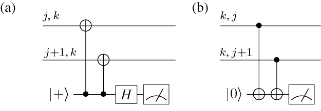
Figure 24. Example of a chain of errors which do not cause any eigenvalue changes in the surface. If errors connect boundaries to other boundaries, the error correction protocol will not detect them. In the case of a 'clean' surface, these error chains are invariants of the surface code. When computation is considered, qubit information are artificial boundaries within the surface. Hence if error chains connect these information qubits to other boundaries, logical errors occur.
Download figure:
Standard image High-resolution image
As we showed in section 10, standard concatenated coding techniques allow for an error rate suppression which scales with the concatenation level as a double exponential while the resource increase scales exponentially. For the surface code, the error rate suppression scales exponentially while the resource increase scales linearly. While these scaling relations might be mathematically equivalent, the surface code offers much more flexibility at the architectural level. Being able to increase the error protection in the computer with only a linear change in the number of physical qubits is far more beneficial than using an exponential increase in resources when utilizing concatenated correction. Specifically, consider the case where an error protected computer is operating at a logical error rate which is just above what is required for an algorithm. If concatenated error correction is employed, then adding another layer of correction will not only increase the number of qubits by an exponential amount, but it will also drop the effective logical error rate far below what is actually required. In contrast, if surface codes are employed, we increase the qubit resources by a linear factor and drop the logical error rate sufficiently for successful application of the algorithm.
We now leave the discussion regarding topological correction models. We emphasize again that this was a very broad overview of the general concept of topological codes. There are many details and subtleties that we have deliberately left out of this discussion and we urge the reader, if interested, to refer to the referenced articles for a more thorough treatment of this topic.
15. Conclusions and future outlook
This review has hopefully provided a basic introduction to some of the most important theoretical aspects of QEC and fault-tolerant quantum computation. The ultimate goal of this discussion was not to provide a rigorous theoretical framework for QEC and fault-tolerance, but instead attempted to illustrate most of the important rules, results and techniques that have evolved out of this field. Hopefully this introduction will serve as a starting point for individuals introducing themselves to this topic. For those wishing to continue research into the QEC field, we highly recommend consulting the papers referenced throughout this review and especially references [Got97, NC00, Got02, KLA+02, Ste01, Got09] which provide a more mathematically rigorous review of QEC and fault-tolerance.
We have not only covered the basic aspects of QEC through specific examples, but also briefly discussed how physical errors influence quantum computation and how these processes are interpreted within the context of QEC. One of the more important aspects of this review is the discussion related to the stabilizer formalism, circuit synthesis and fault-tolerant circuit construction. Stabilizers are arguably the most useful theoretical formalism in QEC as once it is sufficiently understood, most of the important properties of error correcting codes can be investigated and understood largely by inspection.
The study of QEC and fault-tolerance is still an active area of QIP research. Although the library of quantum codes and error correction techniques is vast there is still a significant disconnect between the abstract framework of quantum coding and the more physically realistic implementation of error correction for large-scale quantum information processing.
There are several future possibilities for the direction of quantum information processing. Even with the development of many of these advanced techniques, the physical construction and accuracy of current qubit fabrication is still insufficient to obtain any benefit from QEC. Many in the field now acknowledge that the future development of quantum computation will most likely split into two broad categories. The first is arguably the more physically realistic, namely small qubit applications in quantum simulation. Beyond these smaller qubit applications, we move to truly large-scale quantum computation, i.e. implementing large algorithms such as Shor on qubit arrays well beyond 1000 physical qubits. This would undoubtably require active techniques in error correction. Future work needs to focus on adapting the many codes and fault-tolerant techniques to the architectural level. As we noted in section 10.4, the implementation of QEC at the design level largely influences the fault-tolerant threshold exhibited by the code itself. Being able to efficiently incorporate both the actual quantum code and the error correction procedures at the physical level is extremely important when developing an experimentally viable, large-scale quantum computer.
There are many differing opinions within the quantum computing community as to the future prospects for quantum information processing. Many remain pessimistic regarding the development of a million qubit device and instead look towards quantum simulation in the absence of active error correction as the realistic goal of quantum information. However, in the past few years, the theoretical advances in error correction and the fantastic speed in the experimental development of few qubit devices continues to offer hope for the near-term construction of a large-scale computer, incorporating many of the ideas presented within this review. While we could never foresee the possible successes or failures in quantum information science, we remain hopeful that a large-scale quantum computer is still a goal worth pursuing.
Acknowledgments
The authors wish to thank A M Stephens, R Van Meter, A G Fowler, L C L Hollenberg and A D Greentree for helpful comments and acknowledge the support of MEXT, JST and FIRST projects.
Footnotes
- 3
Worst case fidelity assumes that the state |ψ〉L is orthogonal to the state σxσxσx|ψ〉L.
- 4
Degenerate quantum codes are ones where different types of errors have the same effect on the codestates.
- 5
In general, for an n qubit system, the total dimensionality of the Hilbert space is 2n. If a stabilizer set is defined over this system containing k multiplicativity independent generators, then the dimension of the subspace is 2n−k and therefore the stabilizer set defines a subspace containing n − k logical qubits.
- 6
An operator, U, which is both Hermitian and unitary can only have eigenvalues of ±1.
- 7
The stabilizer formalism was introduced after the 5-qubit code.
- 8
This assumption is for demonstration purposes. In reality, all qubits will experience errors and hence Ej can be of higher weight (up to a weight N operator on an N qubit system). The ability of the error correction code to correct for higher weight errors depends on how all these Ej map the ancilla states under UQEC.
- 9
A degenerate quantum code is one where multiple unique errors can map to the same state; in the case of equation (60) this would mean two operators Ej and E'j, under the unitary UQEC map |A0〉X and |A0〉Z to the same ancilla state.
- 10
If U is not a member of the Clifford group (operators which map Pauli operators to Pauli operators) then E will map to a linear combination of Pauli errors.
- 11
It should be noted that this process is equivalent to directly coupling qubits with quantum gates and then measuring one of the qubits, hence errors will be copied in the same manner as direct coupling.
- 12
Provided we are in eigenstates of
 we can, in principal, be in superpositions of eigenstates of the operators in
. However, the error correction procedure for the BS code projects us back to eigenstates of the gauge operators.
we can, in principal, be in superpositions of eigenstates of the operators in
. However, the error correction procedure for the BS code projects us back to eigenstates of the gauge operators. - 13
It should be noted that for higher distance BS codes, specifically for d ⩾ 5, multiple measurements for each syndrome are required to ensure fault-tolerance.
- 14
The reduction is not exactly p as there is a combinatorial factor that accounts for all the extra error chains that are now possible.