
Abstract
A version of cascaded systems analysis was developed specifically with the aim of studying quantum noise propagation in x-ray detectors. Signal and quantum noise propagation was then modelled in four types of x-ray detectors used for digital mammography: four flat panel systems, one computed radiography and one slot-scan silicon wafer based photon counting device. As required inputs to the model, the two dimensional (2D) modulation transfer function (MTF), noise power spectra (NPS) and detective quantum efficiency (DQE) were measured for six mammography systems that utilized these different detectors. A new method to reconstruct anisotropic 2D presampling MTF matrices from 1D radial MTFs measured along different angular directions across the detector is described; an image of a sharp, circular disc was used for this purpose. The effective pixel fill factor for the FP systems was determined from the axial 1D presampling MTFs measured with a square sharp edge along the two orthogonal directions of the pixel lattice. Expectation MTFs were then calculated by averaging the radial MTFs over all possible phases and the 2D EMTF formed with the same reconstruction technique used for the 2D presampling MTF. The quantum NPS was then established by noise decomposition from homogenous images acquired as a function of detector air kerma. This was further decomposed into the correlated and uncorrelated quantum components by fitting the radially averaged quantum NPS with the radially averaged EMTF2. This whole procedure allowed a detailed analysis of the influence of aliasing, signal and noise decorrelation, x-ray capture efficiency and global secondary gain on NPS and detector DQE. The influence of noise statistics, pixel fill factor and additional electronic and fixed pattern noises on the DQE was also studied. The 2D cascaded model and decompositions performed on the acquired images also enlightened the observed quantum NPS and DQE anisotropy.
Export citation and abstract BibTeX RIS

Original content from this work may be used under the terms of the Creative Commons Attribution 3.0 licence. Any further distribution of this work must maintain attribution to the author(s) and the title of the work, journal citation and DOI.
1. Introduction
Metrics such as presampling modulation transfer function (MTF), noise power spectrum (NPS) and detective quantum efficiency (DQE) are commonly used to describe detector imaging performance. They can be considered as summary measures, of great utility when making comparisons between different detectors, but they may fail to provide information about the potential causes of image quality degradation. In practice, the x-ray signal and noise are transferred through a cascade of multiple amplification and gain stages that can be described with linear system theory and make up the quality of an image (Rabbani et al 1987, Cunningham et al 1994, Cunningham and Shaw 1999, Liaparinos et al 2013, Zhao et al 2015). Cascaded models cover the conversion and interaction steps of x-ray photons and associated secondary particles, from the x-ray quanta fluence incident on the x-ray converter layer to the digital image consisting of an array of pixels. They use gain and scattering processes to model the underlying conversion and transport of particles within the detector and relate the MTF, NPS and DQE to physical detector parameters. A number of authors have developed cascaded models for different types of detectors such as direct- and indirect-conversion digital radiography (DR) (Zhao and Rowlands 1997, Cunningham et al 2002, Gallas et al 2004, Zhao et al 2004), computed radiography (CR) (Hillen et al 1987, Vedantham and Karellas 2010), and more recently photon counting (PC) systems (Tanguay et al 2013, Tanguay et al 2015, Xu et al 2014).
More information on image noise generation may be obtained by splitting the noise into its three main sources: quantum, electronic and fixed pattern components (Evans et al 2002, Mackenzie and Honey 2007, Monnin et al 2014). Detailed studies have shown how detector parameters such as detector composition and thickness affect the noise sources in relation to the detector air kerma and beam quality (Tkaczyk et al 2001, Mackenzie et al 2014). One aspect of cascaded analysis that has not been developed in particular detail is the separation of quantum noise into correlated and uncorrelated components at different stages within the detector and hence the study of these elements is the principal aim of this paper. To achieve this, a new procedure is implemented to measure the 2D presampling MTF and expectation MTF (EMTF) as first described by Dobbins (1995). The 1D mean radial MTF and radial EMTF curves that follow from our method are then used to perform two distinct decompositions of the quantum NPS: into the correlated and uncorrelated components and into the presampling and aliased parts. This distinction between colored and white quantum noises enables the investigation of several key parameters in the cascaded model, such as the Poisson excess noise, the x-ray absorption efficiency and the global secondary gain. In the second part of the work, the DQE is decomposed using the cascaded signal and noise components into successive stages: primary capture, conversion and spreading, secondary capture (coupling), collection and sampling. The influence of additional noise sources such as electronic and fixed pattern noise on DQE (relative to quantum noise) is then investigated using the RN factor defined by Nishikawa and Yaffe (1990). Finally, the NPS and DQE are calculated in 2D across the Fourier plane and compared to measured data in order to examine signal and noise anisotropy for selected systems.
2. Background and theoretical development
Advanced models for the signal and noise transfer through cascaded linear detector models have been already developed for CR systems (Vedantham and Karellas 2010), for scintillation phosphors (Siewerdsen et al 1997, Cunningham et al 2004, Kim 2006) and a-Se (Zhao and Rowlands 1997, Hunt et al 2007), and were recently extended to photon counting (Tanguay et al 2013, Xu et al 2014, Tanguay et al 2015) detectors. In these approaches, signal and noise can be transferred through three types of stages: (1) a gain stage represented as a binary selection process, (2) a stochastic blurring stage represented as a convolution integral with the point spread function (PSF) and (3) a deterministic blurring stage such as an integration over the pixel aperture (Rabbani et al 1987, Cunningham and Shaw 1999). For a gain stage 'i', for input signal amplitude and input NPS respectively di−1 and NPSi−1, the output signal amplitude and NPS will be noted as di and NPSi. The signal amplitude and NPS transfer through a gain stage of mean gain gi and gain variance  can be stated as


For a stochastic blur stage characterized by a convolution process with a PSF, and where Ti(fx, fy) is the Fourier transform of the PSF for the stage 'i', the resulting signal and NPS are given by (Rabbani et al 1987):


For a deterministic blur stage, the NPS transfer is simpler (Cunningham et al 1995):

The detective quantum efficiency (DQE) at stage 'i' was calculated according to its usual definition for images linearized in x-ray fluence units (Q) (IEC 2005):

The signal and noise propagations of an incident x-ray fluence Q through the x-ray detectors were modeled by dividing the detection chain into seven successive elementary stages. The stages 1 to 5 prior sampling have already been extensively described in the literature and are therefore not explicitly derived. The mean output signal, quantum NPS and DQE for these stages are given in table 1 for an image whose pixel values are expressed in incident quantum fluence (Q) unit. The (sampling) stage 6 is developed in detail.
Table 1. Mean signal gain, mean quantum NPS gain and DQE for images expressed in primary quanta values (Q) at the different stages of the cascaded model of x-ray detector.
| Stage | Type | Mean signal gain d(fx, fy)/Q | Mean quantum NPS gain NPSq(fx, fy)/Q | DQE(fx, fy) |
|---|---|---|---|---|
| 1. Capture of incident x-rays | Stochastic gain α |  |
 |
 |
| 2. Conversion of x-rays into secondary quanta | Stochastic gain β |  |
 |
 |
| 3. Spread of secondary quanta | Stochastic spreading T |  |
 |
 |
| 4. Capture of secondary quanta | Stochastic gain κ |  |
 |
 |
| 5. Collection of secondary quanta | Stochastic gain η and deterministic spreading |  |
 |
 |
| 6. Sampling | Aliasing |  |
 |
 |
2.1. Capture of incident x-rays by the detector converter
This is a stochastic gain stage with a gain (probability of x-ray capture or primary detection efficiency) α and gain variance α(1 − α) (binary selection process).
2.2. Conversion of x-rays into secondary quanta
This describes the stochastic gain conversion of x-rays into secondary quanta (light quanta or electronic charges for a-Se or PC detectors): gain β and gain variance  . The fluctuations in this gain term are caused by two principal factors (Swank 1973). First, the use of a polyenergetic spectrum gives a variation in x-ray photon energy which then leads to a variation in generated light or charge—even if there is no variability in light or charge gain per interaction. Moreover, stochastic variations in this conversion gain add additional variability. The variation in the absorbed energy distribution (AED) has been called radiation Swank noise, i.e. the distribution of the amount of energy absorbed in the detector for each interacting x-ray photon, while optical Swank noise represents the variation in the optical pulse distribution (OPD), i.e. the distribution of the number of optical photons detected for each unit of energy absorbed in a scintillator (Swank 1973, Chan and Doi 1984). Note that Swank initially developed these ideas for x-ray scintillators but the gain variability also applies to photoconductors leading to a variation in charge produced per x-ray photon (Fahrig, Rowlands and Yaffe 1995). For PC systems, a noise factor ISPC, equal to the probability that a true photon count is recorded given an interaction event (true positive fraction), was recently introduced, based on a depth dependent interaction statistical model (Tanguay et al 2013). Its effect on noise and DQE is similar to the Swank factor and was thus not distinguished from the Swank factor in this study. The noise associated with this gain stage is described by the Swank factor As (Cunningham et al 1994)

2.3. Spreading of secondary quanta within the converter
This stage represents stochastic spreading of secondary quanta in the detector described in the frequency domain by multiplication with a transfer function describing the scatter spreading characteristics of the detector converter (T) (scintillator or photoconductive layer).
2.4. Capture of secondary quanta (optical or electrical coupling)
This is a stochastic stage that describes the optical or electrical coupling of the x-ray converter to the electronic readout sub-system. The coupling efficiency is a gain stage with a gain κ and gain variance κ (1 − κ) (binary process) which gives the probability that the generated secondary quanta are converted to electronic signal.
2.5. Collection of secondary quanta in the detector elements (pixel aperture)
This is a stochastic gain and deterministic spreading stage with a gain equal to the pixel fill factor  , where Δx and Δy are the detector pixel spacing and ax and ay the pixel aperture (active pixel size) in the x and y directions, and gain variance η (1 − η) (binary process). The spreading is determined by the rectangular pixel aperture and characterized by the modulation transfer function of the pixel using the spatial frequency domain description.
2.6. Sampling
Stage 6 describes the sampling of signal and noise by the pixel lattice and is developed here. The sampling action causes signal and noise spectra to be replicated, with a replicate centred on every harmonic of the sampling frequency 1/a, where a is the pixel pitch. Noise after sampling consists of the infinite sum of aliased presampling NPS centred at the frequencies k/Δx and k/Δy. The noise components with frequency greater than the Nyquist frequency get aliased into the image noise at lower frequencies. The mean sampled signal at stage 6 can be obtained from the respective expressions for stage 5 (table 1) by multiplication with an infinite train of δ functions, uniformly spaced by intervals equal to the pixel sampling (Giger, Doi and Metz 1984):
The product between the converter transfer function T and the pixel aperture function is equal to the modulus of the presampling optical transfer function (OTFpre):

The digital (sampled) OTF is given by (Giger, Doi and Metz 1984, Dobbins 1995) and corresponds to the digital MTFd:

The expectation value of MTFd averaged over all phases (EMTF) and introduced by Dobbins in 1995 is usually used to describe the digital MTF since it satisfies the stationarity property:

The mean sampled quantum NPS at stage 6 can be obtained using the same formalism:


The coefficient kq1 represents the amplitude of the correlated noise component, and depends on the x-ray absorption efficiency (α) and the Poisson excess noise  which arises if conversion noise is not Poisson-distributed (Mackenzie and Honey 2007). The coefficient kq1 will always be greater than 1. The coefficient kq2 represents the non-correlated noise component and is expected to be close to zero since a large average conversion gain (β) is required to ensure no secondary sink occurs and the DQE scales with the quantum absorption efficiency α.
Zhao and Rowlands (1997) showed for a pixel size (ax) smaller than the pixel spacing (Δx):
and hence for the NPS measured on a 2D detector array, the quantum NPS reduces to:

The OTFd is phase dependent (Giger, Doi and Metz 1984, Dobbins 1995), however the NPS components are averaged over an ensemble of different phase realizations and the modulus of the Fourier transform cancels phase information. The NPS will therefore be phase independent and thus satisfies the condition of stationarity. The average over all possible phases of the modulus of OTFd is the expectation MTF (EMTF) (Dobbins 1995) and hence the NPS for stage 6 can be written as:

While Rossmann (1962) proposed that the quantum NPS should be proportional to the square of the detector MTF, Lubberts (1968) predicted a decorrelation between MTF2 and quantum NPS caused by a variation in shape of the light bursts originated at different depths in fluorescent screens. This decorrelation means that signal and noise are transferred through the detector layer with different efficiencies. Nishikawa, Yaffe and Holmes (1989) introduced the quantum noise transfer function (NTFq) to describe the spatial frequency dependence (shape) of the quantum NPS. The factor Rc was then defined to describe the difference in expected signal (quantified using the MTF2) transfer and quantum noise as a function of spatial frequency. The detector DQE at stage 6 can be expressed using the presampling MTF for signal transfer and the Rc factor:


Here, the quantum noise transfer function NTFq can be expressed using the terminology in equation (17):

For converters with considerable presampling blurring such as scintillators, the signal beyond the Nyquist frequency is largely eliminated before pixel sampling, and there is little or no aliasing and hence the EMTF reduces to the presampling MTF (Dobbins 1995). Presampling spread of secondary quanta forces signal sharing with many pixels and the DQE is approximately independent of fill factor (Cunningham 2000). The quantum NPS is in this case expected to be proportional to the presampling MTF2.


Conversely, for sharp detectors with little or no presampling blurring, as is the case of photoconductors such as a-Se, spread of secondary quanta before sampling is small (i.e.  and
and  ). The presampling NPS extends well above the Nyquist frequency and the pixel pitch is not fine enough to sample this signal sufficiently finely to avoid aliasing. The sampling step folds the noise power present above the Nyquist frequency down below the Nyquist frequency. The sampled quantum NPS will be white. This makes the DQE mostly proportional to the fill factor.


2.7. Additional noise components
Electronic NPS (NPSe) and fixed pattern NPS (NPSfp) are not correlated to quantum NPS and can simply be summed together. These noise components were isolated using the method proposed in a previous study (Monnin et al 2014). The importance of the additional noise sources can be quantified by the factor RN that describes the extent to which the system is quantum limited at a given detector (Nishikawa and Yaffe 1990).


It is important to note that differences have to be taken in account in the cascaded model between indirect-conversion (CsI) and direct-conversion (a-Se and PC) detectors. For photoconductor based detectors (e.g. a-Se) we assume the charge spread is negligible, equivalent to taking T = 1 at stage 3—justified given the intrinsic sharpness of this x-ray conversion material since the spatial distribution of primary electrons is much narrower than the pixel size (FWHM of 1.35 μm at 20 keV for a-Se) (Sakellaris et al 2005 and 2007) and further charge spread is practically eliminated by an electric field. Only K-fluorescence escape from the primary x-ray interaction site and reabsorption at a remote position can blur the signal before the conversion stage (Hajdok et al 2008). The NPS is not modified at this stage and remains white (Zhao and Rowlands 1997). The converter transfer function T for direct-conversion detectors is simply determined by x-rays spreading as charge diffusion is negligible, whereas T is determined by optical scattering for CsI converters.
The expressions derived for the quantum NPS are now examined for detectors used in digital mammography, and curve fitting is used to establish the parameters kq1 and kq2, which respectively represent the correlated and non-correlated quantum noise components for a given x-ray detector.
3. Materials and methods
3.1. Properties of the mammography systems and image acquisition
Six digital mammography systems were included in the study: four flat-panel units, a photon counting system that utilizes a scanned multi-slit geometry and a computed radiography system (CR). Basic technical parameters for the detectors are given in table 2. Images for the noise assessment were acquired as described in a previous study (Monnin et al 2014) at nine detector air kerma (DAK) levels. Target values were 6.25, 12.5, 25, 50, 100, 200, 400, 800 and 1600 μGy. The tube load (mAs) was varied to give the DAK closest to these values.
Table 2. Characteristics of the mammography detectors, acquisition parameters and photon fluences obtained with the AEC settings for a 40 mm PMMA block.
| Detector name | Technology | Pixel pitch (μm) | Tube potential | Anode/filter | Effective energy (keV) | Photon fluence/DAK(mm−2 μGy−1) |
|---|---|---|---|---|---|---|
| Carestream SNP-M1 | single-side needle CR | 49 | 28 kV | Mo/Mo | 19.3 | 5167 |
| GE Essential | CsI/a-Si TFT switch | 100 | 29 kV | Rh/Rh | 21.0 | 6275 |
| Hologic Selenia Dimensions | a-Se/TFT switch | 70 | 29 kV | W/Rh | 21.0 | 6189 |
| IMS Giotto | a-Se/TFT switch | 85 | 28 kV | W/Ag | 21.8 | 6734 |
| Philips MicroDose L30 | Photon counter/Si-wafer | 50 | 29 kV | W/Al | 22.5 | 6884 |
| Siemens Inspiration | a-Se/TFT switch | 85 | 29 kV | W/Rh | 21.0 | 6189 |
The MTF images were acquired with the same beam quality (kV and anode/filter combination) as the images used for the noise assessment, but with a tube-current time product (mAs) set to obtain a target DAK of 200 μGy. In order to reduce the amount of scatter at the detector, the additional filter of 40 mm PMMA at the tube exit was replaced by a 2 mm Al filter for the MTF images, as recommended by the IEC standard (IEC 2005). The 40 mm PMMA and 2 mm Al filters are approximately equivalent in terms of mean spectrum energy for the energy range used in mammography.
Detector air kerma values were then converted to their corresponding total photon fluence (Q) by means of Boone's data (Boone 1998) and used to generate detector response functions in conjunction with mean pixel values (PV) following the methodology given in a previous study (Monnin et al 2014). The photon fluence per unit DAK and the AEC settings obtained for the 40 mm PMMA filter are given in table 2 for the different mammography units. Pixel values of the images used for MTF and NPS calculations were systematically re-expressed in x-ray fluence units by means of a linearization process based upon the system response curve.
3.2. Presampling and expectation modulation transfer functions (MTF and EMTF)
The 1D presampling modulation transfer function (MTF) along the two main orthogonal directions defined by the pixel lattice was established using an angled edge method similar to that of Samei et al (1998). The impulse response was obtained from the image of a 50 × 50 mm tungsten (W) sharp edge, 0.5 mm thick, tilted at about 2° with respect to the pixel grid, and positioned at 60 mm from the chest wall side along the central axis of the x-ray beam, directly on the surface of the x-ray table. The angle of the edge with respect to the pixel grid was calculated using a least squares fit to the edge transition position, obtained by estimating the image gradient in the direction perpendicular to the edge line. The projection of the pixel values along the edge line gave the oversampled edge spread function (ESF). In order to assure a constant sampling distance, the ESF was resampled using a curve interpolated over all the points (without smoothing). The MTF is the zero-frequency normalized modulus of the fast Fourier transform of the line spread function (LSF), the derivative of the ESF. The signal-to-noise ratio (SNR) of the MTF curve decreases gradually as the frequency increases (Cunningham and Reid 1992) and hence an average MTF curve for each system was formed from ten MTF images in order to increase MTF precision at high spatial frequencies.
The 1D MTFs in the directions of the pixel lines and columns were used to find the spatial frequency at which the first minimum of the MTF occurs (f0), from which the two orthogonal effective pixel sizes were determined and the effective fill factor of the pixel (η) for the flat panel systems.

The conventional presampling MTF methods are limited to two orthogonal directions across the detector, yet the NPS is available in two dimensions and hence requires reduction to a 1D curve, either by band averaging for the two orthogonal directions or by using the radially averaged NPS for detectors whose NPS is isotropic. We implemented an alternative approach. A 2D MTF was estimated and then used in combination with the 2D NPS. The method utilises a circular W disc of diameter 50 mm and thickness 0.5 mm in place of the standard square edge. The disc was fabricated in the workshop associated with the physics section using a slow wire electron discharge machining (EDM) method. This gives excellent edge orthogonality, i.e. the 0.5 mm edge is machined at 90° to the large circular disc region. Lateral precision was stated as 10−3 mm. The accuracy of the circular disc for MTF calculation was checked by comparison with a sharp square shaped W plate of the same size (50 × 50 × 0.5 mm) for a system with a well-established isotropic MTF. Maximum difference between the presampling MTF curves obtained with the two test objects for the two orthogonal directions (front-back and left-right directions) was less than 3%.
For a given disc image, a threshold method was used to determine the edge of the circular disc while the disc centre was defined as the centre of gravity of the pixels within the disc perimeter. A radial coordinate positioned at the disc centre was then used to divide the disc into angular portions with the same aperture. The presampling ESF for a given angular section was generated by rearranging the pixel data for the corresponding angular aperture according to their distance from the disc centre, and then uniformly re-sampled with an interpolated curve. The 1D MTFs for the different angles were formed in the same manner as described above. In order to facilitate interpolation to a 2D MTF grid, seventh-order polynomial fits were applied to the measured angular 1D MTFs. The 2D MTF matrix was the sum of the 2N different angular MTFi weighted by the 2N angular cos2N functions according to the formula below, where  is the angular aperture and pitch:

Where 
The cos2N functions sum at any point of the matrix is equal to a constant whose value depends on N. This weighting reduces to the 2D weighting method proposed by Konstantinidis et al (2011) for 2D MTF estimation for the particular case where N = 1. The 2D MTF was finally normalized by its value at zero frequency given by the sum of the series:

An angular aperture and pitch of 2.5° (N = 18) was used for the 2D MTF computations in this study. It represents a reasonable compromise between angular resolution and noise in angular ESFs. The mean radial presampling MTF was obtained by averaging the 2D MTF over all the directions.
For undersampled systems, the sampled angular MTFs are phase dependent and the overlap of aliased frequency components can be considered through the calculation of the expectation MTF (EMTF), the average of the sampled MTFs over all possible phase values. The EMTF for an angle i was calculated by averaging the corresponding angular digital optical transfer function (OTFd—the Fourier transform of the LSF) over all possible radial phase values r0 (Dobbins 1995):

Where  is the radial frequency and
  gives the pixel size in the radial direction. The 2D EMTF matrix was then constructed using the method described for 2D MTF and the mean radial EMTF obtained by averaging the non-isotropic 2D EMTF over all the directions.
The converter scattering function T(fx, fy) was calculated from the presampling MTF and the pixel aperture function (Zhao and Rowlands 1997). For CsI scintillators, this term represents optical blur after the x-ray-light conversion stage while for a-Se photoconductors this term accounts for K-shell layers fluorescence reabsorption before the conversion stage.

The mean radial T function was obtained by averaging the 2D T function over all the directions.
3.3. Quantum NPS decomposition
The 2D noise power spectra (NPS) were calculated and decomposed into their three components (quantum, electronic and fixed pattern NPS) as described in a previous study (Monnin et al 2014). The further decomposition of the quantum NPS (NPSq) into its coloured and white parts was computed numerically by determining the kq1 and kq2 coefficients in equation (17) that provide best match to the measured 1D radially averaged NPSq and EMTF2. An iterative procedure with different kq1 and kq2 coefficients was repeated until the quadratic sum of the errors between equation (17) and NPSq for each frequency bin up to the Nyquist frequency was minimized. The kq1 and kq2 coefficients which gave the smallest least square difference were chosen to calculate the parameters α and βκ. The quantities kq1 and kq2 were supposed constant in the Fourier plane and therefore used to calculate the theoretical 2D NPSq with equation (17) and the 2D DQE with equation (18). These calculated data were then compared to the measured 2D NPSq and DQE.
The quantum NPS decomposition in colored and white quantum components enabled several key parameters in the cascaded model to be calculated: the Poisson excess noise (nex), the x-ray absorption efficiency (α) and the global secondary gain (βκ). The Poisson excess noise is directly related to the Swank factor, as the very small term 1/β was neglected:

The x-ray absorption efficiency α scales with the kq1 noise coefficient, after neglecting the very small term 1/β in equation (13).

The global secondary quantum gain given by the product βκ scales with the inverse of the kq2 noise coefficient, and was estimated from equation (14).

The Swank factors As were taken from values published in the literature for an effective energy around 20 keV: 0.95 for CsI layers (Zhao et al 2004), 0.94 for a-Se converters (Fahrig et al 1995) and 0.98 for the Si-wafer PC detector (Tanguay et al 2010).
4. Results and discussion
4.1. Signal transfer properties
Figures 1(a)–(f) show the mean radial MTF, EMTF and converter transfer function T obtained for the six mammography systems. Presampling blurring due to optical photon scattering reduces the MTF of indirect DR and CR systems compared to direct conversion DR detectors. As the presampling MTF reaches zero at or before the Nyquist frequency, no aliasing occurs for the CR system and only a negligible part of signal is aliased for the GE Essential. The EMTF is therefore strictly equal to the presampling MTF for the CR and closely follows the presampling MTF for the GE Essential. For direct conversion detectors, resolution loss comes primarily from the signal sampling process (deterministic blurring by the pixel aperture) as any presampling blurring from x-ray fluorescence is weak (Que and Rowlands 1995). Substantial aliasing of both signal and noise is therefore expected for this kind of system (Dobbins 1995). This was confirmed by the significant difference between the presampling MTF and EMTF measured for the three a-Se x-ray converter based detectors: Selenia Dimensions, Giotto and Inspiration. The inherent spatial resolution of a-Se is high (Hajdok et al 2006) and the converter transfer function T should remain close to unity even at high spatial frequencies (~20 mm−1). From this we would expect the presampling MTF to follow the pixel sinc aperture closely, and while presampling MTF was certainly closer to the pixel sinc function than for the phosphor based detectors, presampling MTF was some way lower than pixel aperture. One possible explanation is x-ray drift toward the pixels due to the spread of electric field lines (interface trapping blurring) (Zhao et al 2003, Hunt et al 2004). There may also be some presampling filtering intentionally introduced to reduce signal and quantum noise aliasing, which is commonly applied for direct-conversion detectors (Ji et al 1998). The radially averaged presampling MTFs measured for the GE Essential, Siemens Inspiration and Hologic Selenia Dimensions are comparable to MTF curves averaged over the left-right and front-back directions published in an earlier study (Marshall et al 2011). The scanning system is a case apart, since charge sharing between neighboring Si strips blurs the signal in the scan direction but the spatial resolution in this direction is mostly determined by the width of the pre-collimator slit and the continuous source motion during image acquisition while the spatial resolution orthogonal to the scan direction is limited by the detector properties (Lundqvist 2003) (figure 2(a)). The presampling MTF approaches zero at the Nyquist frequency in the front-back direction due to a sufficiently small pixel spacing. The presampling MTF is lower in the scan direction where geometric blurring may not enable the primary event to be located with sub-pixel resolution. Eventually no signal aliasing occurs for this system. MTF anisotropy is also seen for the Inspiration, Giotto and SNP-M1 systems whereas the Essential and Selenia MTFs are nicely isotropic. MTF directionality for the Giotto and Inspiration may be due to an asymmetry in the readout electronics that makes the sensitive area of the pixel non square (figure 2(b)). Anisotropy was expected for the CR system because signal lag and temporal filtering used to reduce aliasing during the readout introduce signal correlation along the (fast) scan read direction. This is absent in the (slow) subscan direction (Rowlands 2002, Vedantham and Karellas 2010) (figure 2(c)).

Figure 1. Signal transfer: radially averaged converter transfer function T, presampling MTF and EMTF. (a) Carestream SNP-M1 (b) GE Essential (c) Hologic Selenia Dimensions (d) IMS Giotto (e) Philips MicroDose L30 (f) Siemens Inspiration.
Download figure:
Standard image High-resolution image
Figure 2. Presampling MTF anisotropy. (a) Philips MicroDose (b) Siemens Inspiration (c) Carestream SNP-M1.
Download figure:
Standard image High-resolution imageThe sensitive pixel area (aperture) is smaller than the pixel pitch for flat panel detectors because of the finite size of the pixel electrode. The pixel aperture in the two orthogonal directions of the pixel lattice makes the presampling MTF reach its first minimum at a spatial frequency slightly greater than the inverse of the pixel pitch—this axial touching point can be used to determine the effective fill factor of the pixel. Figure 3 shows a typical example. This method cannot be applied if the MTF has already fallen to zero above the Nyquist frequency e.g. due to strong optical presampling blurring; the mean pixel aperture (averaged over the two orthogonal directions) and the corresponding fill factors used for flat panel systems in this study are given in table 3. Pixel fill factors estimates were close to 90% for the three a-Se detectors and 72.3% for the Essential. The fill factor for the photon counter system could not be estimated through the presampling MTF because presampling blur makes the MTF touch zero before the Nyquist frequency. Such detectors are not susceptible to aliasing, and the NPSq and DQE are approximately independent of fill factor (Cunningham 2000). Thus an approximation was made and the pixel fill factor was assumed to be equal to 1 in the calculations for this system.
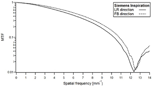
Figure 3. Typical example of the calculation of pixel aperture in the two orthogonal directions of the pixel grid from the first minimums of the presampling MTFs (data: Siemens Inspiration).
Download figure:
Standard image High-resolution imageTable 3. Detector parameters obtained in the study.
| Detector name | Pixel aperture (μm) | Fill factor (η) | Swank factor (As) | Noise coefficient kq1 | Noise coefficient kq2 | Absorption efficiency (α) | Noise excess (nex) | Secondary quantum gain (βκ) |
|---|---|---|---|---|---|---|---|---|
| Carestream SNP-M1 | 48.5 | 1.000 | 0.95 | 1.611 | 0.234 | 0.653 | 0.052 | 6.54 |
| GE Essential | 85 | 0.723 | 0.95 | 1.407 | 0.059 | 0.748 | 0.052 | 43.4 |
| Hologic Selenia Dimensions | 66 | 0.891 | 0.94 | 1.331 | 0.170 | 0.799 | 0.063 | 9.27 |
| IMS Giotto | 80 | 0.896 | 0.94 | 1.372 | 0.309 | 0.775 | 0.063 | 5.20 |
| Philips MicroDose L30 | 50 | 1.000 | 0.98 | 1.350 | 0.221 | 0.756 | 0.021 | 5.99 |
| Siemens Inspiration | 80 | 0.896 | 0.94 | 0.659 | 0.768 | — | 0.063 | — |
4.2. Quantum NPS decomposition
A basic quantum NPS decomposition into the correlated and uncorrelated components has been made using the assumption that quantum noise at the Nyquist frequency was only white and the colored component negligible (i.e. removed by strong presampling blurring) (Evans et al 2002, Mackenzie and Honey 2007). This method is suitable for low-resolution converters with large presampling blurring, but not for a-Se detectors and thus another decomposition method was used. In this study the mean radial EMTF2 curves were used to decompose the quantum NPS into the correlated and uncorrelated components and into the presampling and aliased parts using equation (17) of the cascaded model. The decomposition was successful for the four flat panel systems and the CR. The fitting procedure for the MicroDose system was only successful for the NPSq and EMTF2 measured along the front-back direction; no correlation between quantum noise and EMTF2 or MTF2 could be found in the scan direction. This is due to the fact that there is no relationship between the intrinsic sharpness and noise in the tube motion direction—the MTF in the scan direction is limited by geometrical blurring (the x-ray source motion length and the width of the pre-collimator slit) and is independent of the detector sharpness. The detector resolution and its influence on quantum noise is therefore only seen in the orthogonal direction. The fitted noise coefficients kq1 and kq2 obtained for the different mammography systems are given in table 3. The comparison between the measured and fitted quantum NPS can be seen in figures 3(a)–(f).
The correlated noise coefficient kq1 is related to the x-ray absorption efficiency (α) and Poisson excess noise (nex), and must therefore be greater than 1.

The excess factor describes the increase in quantum noise above the level predicted only on the basis of Poissonian statistics from the number of detected x-rays (Van Metter and Rabbani 1990). Poisson excess noise was found to increase the coloured quantum noise component by 5.2%, 6.3% and 2.1% for the thin needles of Cs-based scintillators (CsI for the GE Essential and CsBr for the Carestream SNP-M1), a-Se (Hologic Selenia Dimensions, Siemens Inspiration and IMS Giotto) and Si-wafer PC (Philips MicroDose) detectors, respectively (table 3). The kq1 noise coefficient for the Siemens Inspiration was however found to be lower than unity, and considering just the conversion processes within the x-ray converter and pixel matrix, this result has no physical meaning. A factor less than one suggests that noise has been reduced by pre-processing or filtering. Some evidence for this explanation comes from the low-frequency bump seen in the measured electronic NPS for this system in a previous study, as electronic noise is expected to be white (Monnin et al 2014). The noise coefficients measured for this system cannot reflect the real detection performance and hence the parameters α, β and κ were not calculated for the Siemens Inspiration.
The x-ray absorption efficiency α calculated from equation (33) includes the x-ray absorption within the detector, but is reduced by the fraction of photons absorbed in the detector protective cover and breast support table, which are expected to be of the order of 10%, and by the fraction of photons that are not photo-absorbed in the converter (the energy deposited when a photon is scattered and does not create a detectable signal). The absorption efficiency α is closely related to the zero frequency DQE. Primary absorption efficiencies between 65.3% (Carestream SNP-M1) and 79.9% (Hologic Selenia Dimensions) were measured for the systems in this study. The x-ray absorption efficiency obtained for the CR system is between the values of 56% measured by Hillen et al for an old powder standard (ST) Fuji CR phosphor layer (1987) and the absorption fraction of 85% measured by Marshall et al (2012) for a needle CsBr layer with coating and support layer for a more recent Agfa HM5.0 plate. The primary absorption efficiency for the Philips MicroDose is also reduced because part of the energy deposited through Compton electrons is rejected when smaller than the electronic discriminator threshold.
The white quantum noise component kq2 scales with 1/β and is expected to be close to zero for all systems. The conversion gain β is of the order 1200 at 20 keV for the CsI (Rowlands 2000) and 400 for a-Se (Zhao and Rowlands 1997). The kq2 coefficients obtained from quantum noise fitting were however all higher than predicted by these values (table 3). It is important to note that the secondary quantum gain β gives the number of secondary quanta produced by absorbed x-ray (and emitted in all directions). The global secondary quantum gain (βκ) calculated from the kq2 noise coefficient (table 3) does however not provide the gain directly following the x-ray interaction but the quantity of electronic signal obtained per x-ray photon absorbed in the converter. This global gain includes only the photons or electrons transported in the forward direction towards the pixel and losses that occur for example in light self-absorption within the scintillator, fiberoptic or lens coupling, absorption and loss of optical quanta within the CCD, secondary quanta scattering or escape in the converter before collection for indirect-conversion detectors. For direct-conversion detectors electron-hole pairs may recombine or be trapped in the x-ray converter, and the final secondary quantum gain will depend on the converter thickness, the applied bias voltage (electric field) and mean-free drift lengths for electrons and holes.
Such analyses are usually represented in quantum accounting diagrams (QAD) (Cunningham et al 1994). If secondary quantum gain β is not sufficiently high to overcome the conversion losses, and the number of light quanta or electronic charges at a given stage falls below that at the primary quantum sink (βκ < 1), a secondary quantum sink occurs (Cunningham et al 1994, Maidment and Yaffe 1994). In this case the uncorrelated quantum noise source becomes important and causes a reduction in DQE, especially at high spatial frequencies (due to the uncorrelated nature of the secondary noise). The global secondary gain was found to be the highest for the GE Essential (βκ = 43.4), and between 5 and 10 for the a-Se and PC detectors, from 5.2 for the Giotto to 9.3 for the Hologic Selenia Dimensions. The secondary gain βκ = 43.4 is higher than the value of 5.5 used in the study of Cunningham et al (2002) to model a CsI-based detector. We could however not find other similar data in the literature for comparison, especially for a-Se based detectors. The secondary gain of 6.54 obtained for the Carestream SNP-M1 system is close to the values already published for a similar needle CR Agfa HM5.0 system, between 6.3 (Marshall et al 2012) and 9, which was estimated by the manufacturer (Leblans et al 2000). The discharge fraction by the readout laser (readout depth) and collection efficiency of the photomultiplier tube are relatively small for CR systems; this reduces quantum gain to a value below 10 and hence these factors become a source of uncorrelated quantum noise on CR images (Rowlands 2002, Vedantham and Karellas 2010).
The white part of quantum noise appears as a constant offset and increasingly gains in importance towards high frequencies. The value of the kq2 coefficient is thus determined by the shape of the NPSq at high frequency, which may be modified by filtering or image pre-processing like low-pass presampling filtering used to reduce quantum noise aliasing for direct conversion detectors. For this reason the effective secondary gains estimated from kq2 coefficients may not reflect true detector performance, in particular for the Siemens. The importance of the uncorrelated NPSq compared to the component correlated to the MTF2 can be appreciated in figures 4(a)–(f). As expected, the correlated NPSq is dominant at low frequency for all the systems, except for the Inspiration. Our results show clearly the amount of white quantum noise is inversely proportional to the secondary quantum gain and becomes an important noise source for detectors with low secondary quantum gain. This link was already shown by Maidment and Yaffe (1994) for mammography detectors optically coupled to CCD. Difference between NPSq and MTF2 increases with frequency and makes the quantum noise transfer function (NTFq) diverge from the MTF, as shown by Lubberts (1968). Loss of correlation between the propagation of signal and noise through the detector can be described by the factor Rc(f) introduced by Nishikawa and Yaffe (1990), as shown in figures 4(a)–(f). As expected, the calculated Rc factors show that the quantum noise transfer (NTFq) is more efficient than the signal transfer (MTF) for all the detectors. The Rc factor may be first lowered by decorrelation between signal and quantum noise before sampling, and then by noise aliasing. The difference between the presampling and sampled Rc factors in figures 4(a)–(f) shows the respective importance of these two effects on signal and quantum noise decorrelation.

Figure 4. Decomposition of NPSq/Q and Rc factor. (a) Carestream SNP-M1 (b) GE Essential (c) Hologic Selenia Dimensions (d) IMS Giotto (e) Philips MicroDose L30 (FB direction) (f) Siemens Inspiration.
Download figure:
Standard image High-resolution imageThe presampling quantum NPS was calculated from equation (37).

The aliased part of quantum NPS is estimated from the difference between formulas (17) and (37). Aliasing increases both the coloured (difference between EMTF2 and MTF2) and white (difference between 1 and  ) components of NPSq. The direct conversion detectors have higher presampling MTFs that cause more noise aliasing than scintillators, resulting in an increased NPS. The aliased quantum NPS gains in importance at higher frequencies, reaching a factor of two greater than the magnitude of the presampling quantum NPS for the a-Se detectors. The quantity of aliased noise was found to be negligible for the Carestream SNP-M1 and Philips MicroDose, and very small for the GE Essential, an indication that these three systems sample finely enough to avoid signal and noise aliasing. Alternatively, one could say that the sampling spacing is well matched to the degree of presampling blurring. The GE Essential has the smallest quantity of aliased noise of the DR systems and the lowest uncorrelated noise of the studied systems. It also follows that this is the unit with the smallest difference between NPSq and MTF2, with the highest Rc factor up to 3.6 mm−1, equal to 1.0 below 1 mm−1. The Hologic Selenia Dimensions have the highest Rc factor for frequencies above 3.6 mm−1.
Regarding the assumptions and limitations of the model used for quantum noise decomposition, our noise model does not consider the effect of the stochastic signal variations caused by the x-ray interaction depth within the scintillators (i.e. the Lubbert's effect). This effect has been investigated for granular (Nishikawa et al 1989, Nishikawa and Yaffe 1990) and columnar phosphors (Badano et al 2004, Kalyvas et al 2015). Neglecting the depth dependence of light emission, MTF and escape efficiency leads an error to the NPS shape at high spatial frequency only, i.e. only the frequency dependency of the quantum noise in EMTF2 may be affected, but not the secondary efficiency coefficients β and κ (Van Metter and Rabbani 1990). Depth dependent blur occurs in columnar CsI as in powder phosphor screens, but not as much. The importance of this effect in our study was estimated from the difference between the presampling  and MTF2, using the calculated presampling Rc factor (figures 4). A maximal low difference of 0.020 and 0.078 was calculated at the Nyquist frequency for the GE Essential (at 5 mm−1) and Carestream SNP-M1 (at 10 mm−1), respectively. The approximation can affect only a small fraction of quantum NPS and is thus not expected to have a practical importance. These two systems have a very low presampling MTF near the Nyquist frequency and the depth dependent blur may hardly result in degradation of DQE at high spatial frequency. Furthermore our measurements have shown that other factors, for example noise aliasing, have a strong influence on the high frequency NPS, especially for systems that have a high MTF at the Nyquist frequency. We therefore think that neglecting the Lubberts effect should only lead to a small increase in the value of the fitted kq2 coefficient, which is determined by the shape of the NPSq at high frequency.
4.3. DQE decomposition
The mean radial quantum DQE measured for the different mammography systems involved in this study were decomposed through the cascaded model (figures 5(a)–(e)). The Siemens data are not reported in this section because the non-physical outcome of the fitting results. The electronic and fixed pattern NPS, taken from a previous study (Monnin et al 2014), were simply added to NPSq to form the total NPS (stage 7). For the Philips MicroDose system, electronic noise was found to be zero and fixed pattern noise was also found to be negligible (less than 1% of total noise, up to the target DAK of 100 μGy). The DQEs measured from the radially averaged MTF and NPS peak at 64% for the GE Essential and Philips MicroDose, 60% for the Hologic Selenia without fixed pattern noise but 50% with, and 48% for the Giotto. The DQEs for the GE Essential and Hologic Selenia Dimensions are in line with DQE curves averaged over the left-right and front-back directions published in previous works: DQE peak at 60% for the GE Essential and 48% for the Hologic Selenia (Marshall et al 2011) and DQE at 0.5 mm−1 was measured at 58% for the GE Essential and 54% for the Hologic Selenia (Mackenzie et al 2014).
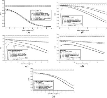
Figure 5. DQE decomposition. (a) Carestream SNP-M1 (b) GE Essential (c) Hologic Selenia Dimensions d) IMS Giotto e) Philips MicroDose L30 (FB direction).
Download figure:
Standard image High-resolution imageThe DQE may be decreased by several factors. Zero-frequency DQE without additional noise sources is given by:

The magnitude of DQE(0) is thus mainly determined by the primary absorption efficiency, but may be further decreased by variations in the statistical processes that govern the production and escape of secondary quanta (Poisson excess noise) and by the global efficiency in producing and collecting secondary quanta, i.e. the mean number of secondary quanta detected per captured x-ray (total secondary efficiency βκη). An ideal detector would have a unity factor kq1 and a factor kq2 equal to zero. The term 1/(βκη2) should be close to zero for a well-designed detector, otherwise a secondary quantum sink develops that degrades the image through the addition of white noise. This is governed by the total secondary quantum gain represented in the cascaded model by the uncorrelated quantum noise coefficient (kq2). A low number of secondary quanta detected per detected x-ray will increase this noise component and lower the DQE. Nishikawa and Yaffe (1990) suggest that the minimum secondary gain should be of the order of secondary quanta (electrons or light photons) per x-ray interaction. The CR system was found to have the lowest zero-frequency DQE (0.55) because of the lowest primary capture efficiency (0.653). The DR systems have zero-frequency DQE between 0.6 and 0.7. The GE Essential is characterized by the highest total secondary gain of the DR systems (43.4) and the absence of noise aliasing, which leads to a zero-frequency DQE reduction of just 5% below the primary capture efficiency.
The DQE decrease with spatial frequency is due to noise aliasing and loss of correlation between signal and noise in the converter. The DQE scales with the Rc factor as shown by equation (18). The loss of correlation between signal and noise makes the MTF lower than NTFq and hence decreases the DQE of the detector at non-zero spatial frequencies.
Only the presampling DQE (DQE at stage 5) represents the simple transfer amplitude of signal to noise ratio (i.e. information) through the imaging system. Thus, the difference between DQE and presampling DQE in figures 5(a)–(e) shows how the DQE is affected by noise aliasing and is a helpful indication of the relative importance of image degradation due to the overlap of the noise. Noise aliasing has two principal effects on DQE: (a) DQE reduction by a constant factor at all spatial frequencies by enhancing the white quantum noise component and (b) DQE reduction increasing with frequency by overlapping the coloured quantum noise components. Aliasing thus reinforces the deleterious effect of the uncorrelated noise on the DQE at all frequencies, and this effect will be relatively more important at high spatial frequency where the presampling DQE is low and may impair the visibility of small objects. The decrease in DQE due to sampling and noise aliasing is thus highest for the a-Se flat panel systems and reaches 0.3 for the Selenia and 0.25 for the Giotto at the Nyquist frequency. Reduction of noise aliasing through presampling blurring is therefore commonly applied for direct-conversion detectors (Ji et al 1998).
The role of the pixel fill factor on the DQE degradation may be also examined using the cascaded model. The GE Essential was found to have the lowest fill factor of the studied systems but this does not negatively affect the DQE—for converter sharpness limited detectors (generally scintillator based), DQE is seen to be largely independent of pixel fill factor (equation (22)). This is in stark contrast to direct-conversion detectors where the DQE scales proportionally to the fill factor. The high fill factors measured for these systems show that special care has to be taken in this parameter for the design of a-Se detectors.
4.4. Anisotropy
For most of the detectors in this study, the 2D measured NPS and DQE showed variations in magnitude that depended on the direction with respect to the detector. According to the cascaded model, quantum noise directionality may be related to the MTF anisotropy through the correlated quantum noise component and to noise aliasing which is anisotropic in the Fourier plane because of differences in pixel size with the direction (EMTF anisotropy). The model explains the sources of NPS and DQE anisotropy and the close agreement from the theory and the measured 2D quantum NPS and DQE is a good indication of the validity of the noise model. Noise anisotropy due to the MTF was seen for the Siemens Inspiration, IMS Giotto and Carestream SNP-M1 systems while the GE Essential and Hologic Selenia Dimensions systems have isotropic MTF shapes and NPS anisotropy that is due to noise aliasing only. Figures 6(a) and (b) compare as an example for the GE Essential the measured 2D quantum NPS to the quantum NPS predicted by the cascaded model. Anisotropy in the NPS only occurs for this system close to the Nyquist frequency since it originates solely from noise aliasing (EMTF anisotropy due to square pixels). Figures 7(a) and (b) show the case of the Giotto with a strong quantum NPS anisotropy. The cascaded model indicates the NPS anisotropy is explained in this case by the MTF anisotropy and the strong noise aliasing. The MTF anisotropy for the IMS Giotto and Siemens Inspiration may be due to an asymmetry in the readout electronics leading to a non-square sensitive area of the pixels. Anisotropic behaviour in the MTF of the Anrad detector, employed in both of these systems, was described by Bissonnette et al (2005). Anisotropy of quantum noise was expected for the CR system because of the differences in MTF along the scan and subscan directions (Rowlands 2002, Vedantham and Karellas 2010). Quantum NPS for the Philips MicroDose shows an anisotropy which is not related to the MTF directionality (the MTF and quantum NPS are not correlated except for the direction orthogonal to the scan) or aliasing (there is almost no aliasing for this system), but is due mostly to the directionality of charge sharing across the detector elements. With charge sharing, photons may be double counted in two adjacent channels of the Si-strip and introduce a correlation that colors the NPS in the front-back direction. In the scan direction, however, the successive readouts are still uncorrelated and the NPS is expected to be more constant along this axis (Lundqvist 2003).

Figure 6. Quantum NPS for the GE Essential. (a) Cascaded model (b) measured.
Download figure:
Standard image High-resolution image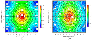
Figure 7. Quantum NPS for the IMS Giotto. (a) Cascaded model (b) measured.
Download figure:
Standard image High-resolution imageBoth uncorrelated quantum noise and noise aliasing cause decorrelation between signal and noise and can make the DQE anisotropic. In their absence, the anisotropy seen in both the MTF and NPSq cancels out in DQE. The uncorrelated NPSq component is, for instance, the only source of DQE anisotropy for the CR system, which is free of aliasing (figures 8(a) and (b)). The opposite situation is seen for the Giotto and Siemens Inspiration: the strong NPS anisotropy originating from the MTF is almost completely removed in the DQE (figures 9(a) and (b) for the Giotto). The Philips MicroDose system is somewhat different in that its DQE shows the strongest anisotropy of all the systems studied. The anisotropy in MTF and NPS do not compensate for each other; geometrical blurring due to the focus motion during the acquisition correlates the signal along the scan direction but not the noise—hence signal and noise are not correlated in this direction. This decorrelation causes a reduction in DQE along the direction of motion compared to the orthogonal direction (figure 10). When measuring the DQE for anisotropic systems, it is important to take the full 2D MTF and NPS in the calculation, for example by computing the 1D MTF and NPS curves by radial averaging. Axial 1D DQE curves may not include the full 2D resolution and noise pattern and noise spikes, and could therefore fail to capture all the SNR properties of the image.

Figure 8. DQE for the Carestream SNP-M1. (a) Cascaded model (b) measured.
Download figure:
Standard image High-resolution image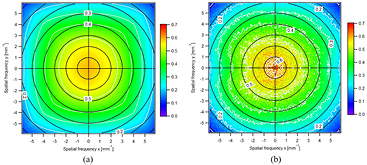
Figure 9. DQE for the Giotto. (a) Cascaded model (b) measured.
Download figure:
Standard image High-resolution image
Figure 10. Measured DQE for the MicroDose.
Download figure:
Standard image High-resolution image
5. Conclusion
This study has introduced and applied a new methodology for measuring of 2D presampling MTF measurement using a circular sharp edge and 2D matrix reconstruction using cosines weightings. This method has shown to be useful for 2D MTF and EMTF computation with any choice of angular pitch, and was successfully applied to compute 2D DQE with an angular precision of 2.5°. Cascaded linear system theory was then used to describe signal and noise characteristics measured on the images acquired on six different digital mammography systems. A methodology was applied to decompose the 2D quantum NPS into the correlated and uncorrelated parts by fitting the 1D radial averaged NPS with the 1D mean radial EMTF2 calculated from the 2D MTF. The pixel fill factors, determined from the minimum point of the presampling MTF along both directions of the pixel lattice, enabled the determination of the aliased part of the quantum NPS, from which the presampling NPS and DQE were calculated. These methods were then successfully used to determine the main physical parameters of the detectors—such as primary absorption fraction and global secondary quantum gain. Knowledge of these parameters gave insight into the magnitude of DQE at low and high spatial frequencies and into DQE anisotropy in the Fourier plane. This study therefore provides a comprehensive model for a 2D analysis of detector performance and quantum noise characterization.