

Abstract
This study aims at developing a joint FDG-PET and MRI texture-based model for the early evaluation of lung metastasis risk in soft-tissue sarcomas (STSs). We investigate if the creation of new composite textures from the combination of FDG-PET and MR imaging information could better identify aggressive tumours. Towards this goal, a cohort of 51 patients with histologically proven STSs of the extremities was retrospectively evaluated. All patients had pre-treatment FDG-PET and MRI scans comprised of T1-weighted and T2-weighted fat-suppression sequences (T2FS). Nine non-texture features (SUV metrics and shape features) and forty-one texture features were extracted from the tumour region of separate (FDG-PET, T1 and T2FS) and fused (FDG-PET/T1 and FDG-PET/T2FS) scans. Volume fusion of the FDG-PET and MRI scans was implemented using the wavelet transform. The influence of six different extraction parameters on the predictive value of textures was investigated. The incorporation of features into multivariable models was performed using logistic regression. The multivariable modeling strategy involved imbalance-adjusted bootstrap resampling in the following four steps leading to final prediction model construction: (1) feature set reduction; (2) feature selection; (3) prediction performance estimation; and (4) computation of model coefficients. Univariate analysis showed that the isotropic voxel size at which texture features were extracted had the most impact on predictive value. In multivariable analysis, texture features extracted from fused scans significantly outperformed those from separate scans in terms of lung metastases prediction estimates. The best performance was obtained using a combination of four texture features extracted from FDG-PET/T1 and FDG-PET/T2FS scans. This model reached an area under the receiver-operating characteristic curve of 0.984 ± 0.002, a sensitivity of 0.955 ± 0.006, and a specificity of 0.926 ± 0.004 in bootstrapping evaluations. Ultimately, lung metastasis risk assessment at diagnosis of STSs could improve patient outcomes by allowing better treatment adaptation.
Export citation and abstract BibTeX RIS
1. Introduction
Soft-tissue sarcomas (STSs) constitute a heterogeneous group of malignant neoplasms of mesenchymal cell origin. More than 50 sub-types are recognized by the World Health Organization (WHO). STSs are relatively uncommon, representing approximately 0.7% of new adult malignancies in the United States (Siegel et al 2014). The majority of new cases are either intermediate or high-grade tumours and may arise in virtually all sites, with the extremities as the most common site of origin (Brennan 2005). In general, the different forms of therapy lead to excellent local control of STSs of the extremities. However, approximately 25% of all patients with STSs develop distant metastases (Billingsley et al 1999). In the case of high-grade tumours specifically, the metastatic rate goes up to approximately 50% (Brennan 2005). The lungs are the main site of metastases with approximately 80% of metastatic cases in STSs of the extremities (Lewis and Brennan 1996). The prognosis of patients who develop lung metastases is generally poor, with a 3-year survival rate of 46% for patients who have undergone surgical resection of lung metastases, and 17% for patients who did not (Billingsley et al 1999). Better systemic therapies at earlier stages are thus needed for the management of STSs of the extremities with risk for lung metastases (Brennan 2005). In this situation, more aggressive chemotherapy regimens or targeted cancer therapy adapted to the histopathology of the tumour could be considered (Komdeur et al 2002). The specific and early evaluation of lung metastasis risk (or prediction of lung metastases) in the course of STS management is therefore of great interest since it could potentially allow for better adapted treatments and consequently, improve overall survival.
Most tumours do not represent a homogeneous entity, but rather are composed of multiple clonal sub-populations of cancer cells forming complex dynamical systems that exhibit rapid evolution as a result of different therapy perturbations. In solid cancers such as STSs, the tremendous extent of heterogeneous characteristics is expressed at multiple levels. Genes, proteins, cellular microenvironments, tissues and anatomical landmarks within tumours exhibit considerable spatial and temporal variations that could potentially yield valuable information about tumour aggressiveness. However, studying tumour heterogeneity using histopathological samples from biopsies is very difficult since the procedure is invasive and the information obtained may vary depending on which part of the tumour is sampled (Longo 2012). This issue is addressed by the new emerging field of 'radiomics', which refers to the extraction and analysis of large amounts of information from medical images using advanced quantitative feature analysis (Kumar et al 2012, Lambin et al 2012). The central hypothesis of radiomics is that the genomic heterogeneity of aggressive tumours could translate into heterogeneous tumour metabolism and anatomy, a concept demonstrated by Segal et al (2007) and Diehn et al (2008), and recently verified by Aerts et al (2014). Diagnostic images could thus reveal important prognostic information about disease risk. In this work, we attempt to quantify intratumoural heterogeneity in STSs using texture analysis performed on 2-deoxy-2-[18F]fluoro-D-glucose (FDG) positron emission tomography (PET) and magnetic resonance imaging (MRI). Figure 1 depicts how functional FDG-PET and anatomical MR imaging information together reflect the heterogeneous sub-region characteristics of aggressive STSs.
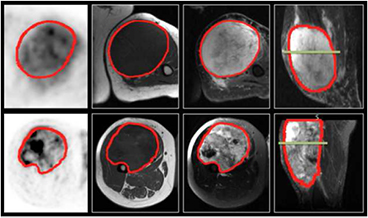
Figure 1. FDG-PET and MRI diagnostic images of two patients with soft-tissue sarcomas of the extremities. Top row: patient that did not develop lung metastases. Bottom row: patient that eventually developed lung metastases. 1st column: FDG-PET images, axial plane. 2nd column: T1-weighted images, axial plane. 3rd column: T2-weighted fat-saturated images, axial plane. 4th column: short tau inversion recovery images, sagittal plane. The green lines in the two images of the 4th column correspond to the plane shown in the three other respective images.
Download figure:
Standard image High-resolution imageThe texture of an image could be globally defined as the spatial arrangement of pixels of different intensities (i.e. gray levels). Texture analysis is concerned with the quantitative description of the spatial distributions of different gray-levels within a region of interest from the extraction of different imaging features. The interest for this method by the radiomics community has grown up rapidly in the last few years, as it is considered to have the potential to extensively characterize the complexity of imaging intensity patterns within tumours (i.e. intratumoural heterogeneity). The association of different texture features with different clinical endpoints (i.e. predictive value) have been previously reported in different cancer sites on single patient cohorts: El Naqa et al (2009), Tixier et al (2011) and Cook et al (2013) using texture features extracted from FDG-PET scans, and Vaidya et al (2012) using texture features separately extracted from FDG-PET and CT scans. More recently, Aerts et al (2014) assessed the prediction performance of a prognostic radiomics signature extracted from CT scans on multiple patient cohorts of different cancer types, whereas Hatt et al (2015) evaluated the complementarity of a few texture features with the metabolically active tumour volume extracted from FDG-PET scans.
With the emergence of individualized medicine, a growing need exists for the development of clinically-integrated prediction models that support treatment decision-making (Lambin et al 2013). Once useful imaging biomarkers (e.g. texture features) are identified to be relevant prognostic factors of a given tumour outcome, models combining those factors may be constructed to improve outcome prediction performance. Although studies based on single feature response (univariate analysis) can be informative, multivariable models are expected to more comprehensively characterize intratumoural heterogeneity. Considering the high risk of lung metastases in STSs of the extremities and the resulting poor prognosis, the main objective of this work is to develop a joint texture-based multivariable model from pre-treatment FDG-PET and MRI scans for the evaluation of lung metastasis risk at the time of diagnosis of primary STSs of the extremities. This information could eventually assist physicians in their choice of treatment and potentially improve patient survival. Towards this goal, we first investigate if the creation of new composite textures from the combination of FDG-PET and MR imaging information via volume fusion could better identify aggressive tumours. We then develop multivariable modeling strategies for the construction of texture-based models with optimal predictive and generalizability properties from a large number of radiomics features. To our knowledge, this is the first study that explores the potential of texture features for the prediction of lung metastases in STS cancer, and the first study that explores the potential of joint FDG-PET and MRI texture features for the assessment of biological properties of any type of cancer.
2. Materials and methods
To ease reading, some acronyms and definitions frequently used in the text are described in table 1.
Table 1. Acronyms/definitions used in the text.
| Acronym/Definition | Description |
|---|---|
| STS | Soft-tissue sarcoma |
| T1 | T1-weighted |
| T2FS | T2-weighted fat-supression |
| LungMets | Patients that developed lung metastases |
| NoLungMets | Patients that did not develop lung metastases |
| Separate scans | FDG-PET, T1 and T2FS scans |
| Fused scans | FDG-PET/T1 and FDG-PET/T2FS scans |
| SUV | Standard uptake value |
| Global | First-order histogram |
| GLCM | Gray-level co-occurence matrix |
| GLRLM | Gray-level run-length matrix |
| GLSZM | Gray-level size zone matrix |
| NGTDM | Neighbourhood gray-tone difference matrix |
| MRI Inv. | Inversion of MRI intensities |
| MRI weight | Weight given to MRI sub-bands in the fusion process |
| WBPF | Wavelet band-pass filtering |
| Scale | Isotropic voxel size |
| Quant. algo. | Quantization algorithm |
| Ng | Number of gray levels |
| Predictive value | Degree to which a feature is associated to tumour outcome |
| Degree of freedom | Combination of texture extraction parameter types allowed to vary |
| rs | Spearman's rank correlation coefficient |
| AUC | Area under the receiver operating characteristic curve |
2.1. Data
2.1.1. Patient cohort.
Subsequent to research ethics board (REB) approval, a database of 51 patients with histologically proven primary STSs of the extremities (denoted as 'STSs' only for the rest of the text) was retrospectively retrieved. Patients with metastatic and/or recurrent STSs at presentation were excluded from the study. The patient cohort was divided into two groups: (1) 32 patients that did not develop lung metastases (denoted as 'NoLungMets'; median follow-up time of 27 months, range 12–70 months); and (2) 19 patients that developed lung metastases (denoted as 'LungMets'; median follow-up time of 20 months, range 4–31 months) during the follow-up period. Patients from the NoLungMets group with a follow-up time smaller than 12 months were excluded from the study. Lung metastases were either proven by biopsy or diagnosed by an expert physician from the appearance of typical pulmonary lesions on CT and/or FDG-PET images. Table 2 provides summary characteristics of the patient cohort.
Table 2. Characteristics of STS patient cohort.
| Characteristic | Type | No. of patients (%), n = 51 |
|---|---|---|
| Sex | Male | 24 (47) |
| Female | 27 (53) | |
| Age (y) | Range | 16–83 |
| Mean ± STD | 55 ± 17 | |
| Histology | Liposarcoma | 11 (21) |
| Malignant fibrous histiocytomas | 17 (33) | |
| Leiomyosarcoma | 10 (20) | |
| Synovial sarcoma | 5 (10) | |
| Fibrosarcoma | 1 (2) | |
| Extraskeletal bone sarcoma | 4 (8) | |
| Other | 3 (6) | |
| Extremity site | Lower | 47 (92) |
| Upper | 4 (8) | |
| Grade | High | 28 (55) |
| Intermediate | 15 (29) | |
| Low | 5 (10) | |
| Ungraded | 3 (6) | |
| Recurrence/Spread | Distant–Lungs | 19 (37) |
| Distant–Other than Lungs | 6 (12) | |
| Locoregional | 4 (8) | |
| None | 24 (47) | |
| Treatment | Radiotherapy + Surgery | 30 (59) |
| Surgery + Chemotherapy | 7 (14) | |
| Radiotherapy + Surgery + Chemotherapy | 14 (27) |
2.1.2. Imaging data.
All 51 eligible patients had pre-treatment FDG-PET/CT and MRI scans between November 2004 and November 2011. All FDG-PET/CT scans were performed on a PET/CT scanner (Discovery ST, GE Healthcare, Waukesha, WI) at the McGill University Health Centre (MUHC). For the PET portion of the scans, a median of 420 MBq (range: 210–620 MBq) of FDG was injected intravenously. Approximately 60 min following the injection, whole-body 2D imaging acquisition was performed using multiple bed positions, with a median of 180 s (range: 160–300 s) per bed position. PET attenuation corrected images were reconstructed (axial plane) using an ordered subset expectation maximization (OSEM) iterative algorithm. The FDG-PET slice thickness resolution was 3.27 mm for all patients and the median in-plane resolution was 5.47 × 5.47 mm2 (range: 3.91–5.47 mm).
The MRI scans resulted from clinical acquisitions with non-uniform protocols across patients. Twelve patients had their images acquired at the MUHC, and 39 in an outside institution. Three types of MRI sequences routinely used in clinical protocols were selected for the study, namely T1-weighted (T1), T2-weighted fat-saturated and short tau inversion recovery (STIR) sequences. Overall, the median in-plane resolution was 0.74 × 0.74 mm2, 0.63 × 0.63 mm2 and 0.86 × 0.86 mm2 (range: 0.23–1.64 mm, 0.23–1.64 mm and 0.23–1.72 mm pixel width), and the median slice thickness was 5.5 mm, 5.0 mm and 5.0 mm (range: 3.0–10.0 mm, 3.0–8.0 mm and 3.0–10.0 mm) for T1, T2-weighted fat-saturated and STIR scans, respectively. T1 sequences were acquired in the axial plane for all patients. On the other hand, patients were scanned in different planes with either or both T2-weighted fat-saturated and STIR sequences, which macroscopically are both T2-weighted sequences aiming to supress the fat signal in the body. From a texture point of view, T2-weighted fat-saturated and STIR images are considered similar, and they were thus combined in the same scan category with only one of the two sequences used per patient. T2-weighted fat-saturated scans were selected by default due to their higher axial scan availability (n = 26). When T2-weighted fat-saturated scans were not available, STIR scans were used (n = 25). For the rest of the text, this category of scans is referred to as T2FS (T2-weighted fat-suppression) scans.
2.2. Tumour volume definition
Contours defining the 3D tumour region for each patient were manually drawn slice-by-slice on T2FS scans by an expert radiation oncologist. For patients with visible edema in the vicinity of the tumours (n = 32), two contours were drawn: one incorporating the visible edema and one excluding it, as shown in figure 2. Contours were propagated to FDG-PET and T1 scans using rigid registration with the commercial software MIM® (MIM software Inc., Cleveland, OH). The results presented in this work were obtained from texture analysis performed on the volume of interest of each patient as defined by the contour containing no edema.
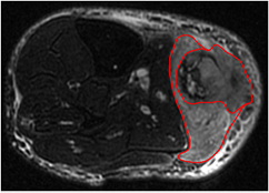
Figure 2. Example of soft-tissue sarcoma tumour volume definition performed on the T2-weighted fat-saturated scan of a patient of the LungMets group. The inner contour exclude visible edema in the vicinity of the tumour.
Download figure:
Standard image High-resolution image2.3. Imaging data pre-processing
Prior to texture analysis, FDG-PET and MRI DICOM data were transferred into MATLAB® (The MathWorks Inc., Natick, MA) format using the software CERR (Deasy et al 2003). All subsequent analyses were performed in MATLAB®. FDG-PET scans were first converted to standard uptake value (SUV) maps, followed by the application of a square-root transform to help in the stabilization of the PET noise in the images. MRI scans were kept in raw data form, and voxels within the tumour region with intensities outside the range μ ± 3σ were rejected and not considered in subsequent texture computations, as suggested by Collewet et al (2004) for making MRI texture measurements more reliable.
2.4. FDG-PET/MR volume fusion
The fusion of FDG-PET and MRI volumes first starts with the registration of the scans as described in section 2.2. The 3D discrete wavelet transform (DWT) is then used to combine the spatial and frequency characteristics of the two modalities as follows:
- (i)Downsample the MRI volume (raw data, no pre-processing) to the resolution of the FDG-PET volume (pre-processed, see section 2.3) using cubic interpolation. Normalize the intensity range of FDG-PET and MRI tumour regions between 0 and 255. Invert MRI intensities if needed.
- (ii)Apply the 3D DWT to the FDG-PET and MRI volumes up to one decomposition level using the wavelet basis function symlet8.
- (iii)Apply the μ ± 3σ normalization scheme (see section 2.3) respectively to the wavelet coefficients of the tumour region of the different MRI sub-bands. The rejected MRI wavelet coefficients are then replaced by the spatially corresponding coefficients of the FDG-PET sub-bands.
- (iv)Perform a weighted average of the spatially corresponding wavelet coefficients of all PET and MRI sub-bands to obtain a single set of fused wavelet coefficients. If the weight given to MRI wavelet coefficients is denoted as 'MRI weight' and the weight given to PET wavelet coefficents is denoted as 'PET weight', MRI weight ranges from 0 to 1 and PET weight = 1 − MRI weight.
- (v)Apply the 3D inverse DWT to the set of fused wavelet coefficients using the reconstruction wavelet basis function symlet8 to obtain a fused FDG-PET/MRI tumour volume.
The choice of the wavelet basis function symlet8 is based on our previous work (Vallières 2013), in which that basis function was shown to produce fused textures with best predictive value. This could be explained from the fact that symlets is a family of orthogonal and compactly supported wavelets with the least asymmetry and highest number of vanishing moments for a given support width, which would help in the local preservation of spatial characteristics of images.
The fusion process yields two new types of scans: FDG-PET/T1 and FDG-PET/T2FS. We also tested if the inversion of MRI intensities prior to fusion with FDG-PET could enhance texture characteristics in the fused volumes. Figure 3 shows an example of the fusion of FDG-PET and T2FS scans for a patient of the LungMets group.

Figure 3. Example of the fusion (middle) of a T2-weighted fat-saturated scan (left) and a FDG-PET scan (right) with a MRI weight value of 0.5, for a patient of the LungMets group. The T2-weighted fat-saturated scan was registered and downsampled to the FDG-PET scan resolution and is presented in raw data format (no pre-processing). The FDG-PET scan is presented in pre-processed format. The intensity range of the 3D tumour region of the three scans was normalized between 0 and 255.
Download figure:
Standard image High-resolution image2.5. Feature extraction
The methodology used to extract the imaging features from the tumour region of the pre-treatment FDG-PET and MRI scans is described below.
2.5.1. Non-texture features (9).
In total, nine non-texture features were extracted for completeness.
SUV metrics (5).
Five non-texture features were extracted from the tumour region of the FDG-PET scans.
- (i)SUVmax: Maximum SUV of the tumour region.
- (ii)SUVpeak: Average of the voxel with maximum SUV within the tumour region and its 26 connected neighbours.
- (iii)SUVmean: Average SUV value of the tumour region.
- (iv)AUC-CSH: Area under the curve of the cumulative SUV-volume histogram describing the percentage of total tumour volume above a percentage threshold of maximum SUV (Van Velden et al 2011).
- (v)Percent Inactive: Percentage of the tumour region that is inactive. A threshold of 0.005 × (SUVmax)2 followed by closing and opening morphological operations were used to differentiate active and inactive regions on FDG-PET scans.
Volume.
Number of voxels in the tumour region extracted from T2FS scans multiplied by the dimension of voxels.
Size.
Longest diameter of the tumour region extracted from T2FS scans.
Solidity.
Ratio of the number of voxels in the tumour region to the number of voxels in the 3D convex hull of the tumour region (smallest polyhedron containing the tumour region). This metric is extracted from T2FS scans.
Eccentricity.
The ellipsoid that best fits the tumour region is first computed using the framework of Li and Griffiths (2004). The eccentricity is then given by [1 − a × b/c2]1/2, where c is the longest semi-principal axes of the ellipsoid, and a and b are the second and third longest semi-principal axes of the ellipsoid.
2.5.2. Texture features (41).
In total, 41 texture features were extracted from the tumour regions of 5 different types of scans: FDG-PET, T1 and T2FS scans ('separate scans'), and FDG-PET/T1 and FDG-PET/T2FS scans ('fused scans'). Table 3 presents the list of texture features used in this study. Global features are extracted from the intensity histogram of the tumour region, whereas GLCM, GLRLM, GLSZM and NGTDM textures are matrix-based features. In this work, histograms with 100 bins were used for the computation of Global features. GLCMs, GLRLMs, GLSZMs and NGTDMs were constructed using 3D analysis of the tumour region with 26-voxel connectivity. Only one GLCM, GLRLM, GLSZM and NGTDM was computed per scan by simultaneously taking into account the neighbouring properties of voxels in the 13 directions of 3D space. However, the 6 voxels at a distance of 1 voxel, the 12 voxels at a distance of  voxels, and the 8 voxels at a distance of
  voxels around center voxels were treated differently in the calculations of the GLCMs, the GLRLMs and the NGTDMs in order to take into account discretization length differences (assuming that resampling to isotropic voxel size is applied beforehand, see section 2.5.3). Detailed description and methodology employed to extract the 41 texture features is available in supplementary appendix A (stacks.iop.org/PMB/60/145471/mmedia).
Table 3. Texture features used in this study.
| Texture type | Reference(s) | Texture name |
|---|---|---|
| Global | — | Variance |
| Skewness | ||
| Kurtosis | ||
| GLCM |
(Haralick et al 1973) | Energy |
| Contrast | ||
| Correlation | ||
| Homogeneity | ||
| Variance | ||
| Sum Average | ||
| Entropy | ||
| GLRLM |
(Galloway 1975) | Short Run Emphasis (SRE) |
| Long Run Emphasis (LRE) | ||
| Gray-Level Non-uniformity (GLN) | ||
| Run-Length Non-uniformity (RLN) | ||
| Run Percentage (RP) | ||
| (Chu et al 1990) | Low Gray-Level Run Emphasis (LGRE) | |
| High Gray-Level Run Emphasis (HGRE) | ||
| (Dasarathy and Holder 1991) | Short Run Low Gray-Level Emphasis (SRLGE) | |
| Short Run High Gray-Level Emphasis (SRHGE) | ||
| Long Run Low Gray-Level Emphasis (LRLGE) | ||
| Long Run High Gray-Level Emphasis (LRHGE) | ||
| (Thibault et al 2009) | Gray-Level Variance (GLV) | |
| Run-Length Variance (RLV) | ||
| GLSZM |
(Galloway 1975) | Small Zone Emphasis (SZE) |
| Large Zone Emphasis (LZE) | ||
| (Thibault et al 2009) | Gray-Level Non-uniformity (GLN) | |
| Zone-Size Non-uniformity (ZSN) | ||
| Zone Percentage (ZP) | ||
| (Chu et al 1990) | Low Gray-Level Zone Emphasis (LGZE) | |
| (Thibault et al 2009) | High Gray-Level Zone Emphasis (HGZE) | |
| (Dasarathy and Holder 1991) | Small Zone Low Gray-Level Emphasis (SZLGE) | |
| Small Zone High Gray-Level Emphasis (SZHGE) | ||
| (Thibault et al 2009) | Large Zone Low Gray-Level Emphasis (LZLGE) | |
| Large Zone High Gray-Level Emphasis (LZHGE) | ||
| (Thibault et al 2009) | Gray-Level Variance (GLV) | |
| Zone-Size Variance (ZSV) | ||
| NGTDM |
(Amadasun and King 1989) | Coarseness |
| Contrast | ||
| Busyness | ||
| Complexity | ||
| Strength |
aGLCM: Gray-level co-occurence matrix. bGLRLM: Gray-level run-length matrix. cGLSZM: Gray-level size zone matrix. dNGTDM: Neighbourhood gray-tone difference matrix.
2.5.3. Texture extraction parameters (6).
The influence of the following six extraction parameters on the predictive value of textures was investigated.
Fusion parameters (2).
The following two parameters apply only to fused scans (FDG-PET/T1 and FDG-PET/T2FS scans):
- (i)Inversion of MR imaging intensities in the FDG-PET/MRI fusion process (see section 2.4). This parameter is denoted as 'MRI Inv'. MRI Inv. of 0 and 1 (no inversion/inversion) were tested.
- (ii)Weight applied to MRI wavelet sub-bands in the FDG-PET/MRI fusion process (see section 2.4). This parameter is denoted as 'MRI weight'. MRI weight values of
 , , , and were tested in this work.


Wavelet band-pass filtering (1).
This parameter is denoted as 'WBPF'. This operation is carried out by applying a different weight to band-pass sub-bands (LHL, LHH, LLH, HLL, HHL and HLH) of the tumour region as compared to low- and high-frequency sub-bands (LLL and HHH) in the wavelet domain. The ratio of the weight applied to band-pass sub-bands to the weight applied to the other sub-bands is defined by R. Ratios of  ,
,  , 1,
, 1,  and 2 were tested.
Isotropic voxel size (1).
This parameter is denoted as 'Scale'. Prior to the computation of texture features, all volumes were resampled to an isotropic voxel size set to a desired resolution using cubic interpolation. Scale values of 1 mm, 2 mm, 3 mm, 4 mm, 5 mm and initial in-plane resolution (denoted 'in-pR') were tested. For example, if the desired Scale was set to 5 mm, a FDG-PET volume with voxel size of 5.47 × 5.47 × 3.27 mm3 would be isotropically resampled to a voxel size of 5 × 5 × 5 mm3. If the desired Scale was set to in-pR, a MRI volume with voxel size of 0.86 × 0.86 × 5 mm3 would be isotropically resampled to a voxel size of 0.86 × 0.86 × 0.86 mm3. Note that Global texture features are extracted after isotropically resampling to the in-plane resolution without further processing.
Quantization of gray levels (2).
Prior to the computation of texture features, the full intensity range of the tumour region was quantized to a smaller number of gray levels Ng. The quantization process maps the voxel values of a volume to a finite set  of reconstruction levels by defining a set
  of decision levels. Two extraction parameters are related to the quantization of gray levels in the volumes:
- (i)Quantization algorithm. This parameter is denoted as 'Quant. algo'. Equal-probability and Lloyd-Max quantization algorithms were implemented in this work using the functions histeq and lloyds of MATLAB®, respectively. Equal-probability quantization attempts to define decision thresholds in the volume such that the number of voxels with reconstructed level rk is the same in the quantized volume for all k (i.e. for all gray levels), whereas Lloyd-Max quantization attempts to minimize the mean-squared quantization error of the output (Max 1960, Lloyd 1982).
- (ii)Number of gray levels (Ng) in the quantized volume. Ng of 8, 16, 32 and 64 were tested.
Texture extraction summary.
Considering the full set of texture extraction parameters of Global features and higher-order texture features (GLCM, GLRLM, GLSZM and NGTDM), a total of 27 405 and 182 700 scan-texture-parameter combinations were computed in this work for separate and fused scans, respectively. Figure 4 presents a summary of the workflow of extraction of texture features.
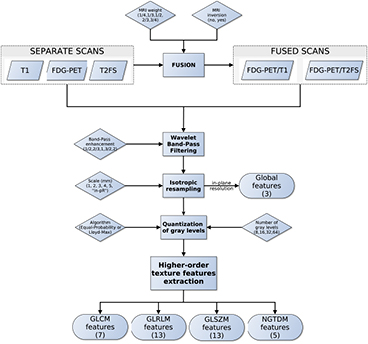
Figure 4. Workflow of extraction of texture features.
Download figure:
Standard image High-resolution image2.6. Univariate analysis
Univariate association between the whole set of features (9 non-texture features and 210 105 scan-texture-parameter features) and lung metastases development in STSs was investigated using Spearman's rank correlation (rs). To correct for multiple tests comparisons, the Bonferroni correction method was applied: the significance level was lowered to a value p < α/K, where K is the number of comparisons and α the significance level set to 0.05.
2.7. Multivariable analysis
The process of combining features into a multivariable model was achieved using the logistic regression utilities of the software DREES (El Naqa et al 2006). We are interested in finding a linear combination of p variables such that the multivariable model of interest takes the form:

where the vector of input variables (imaging data) of the ith patient is  , for a number N of patients. The set
  is the set of regression coefficients of the model to be determined such that the conditional probability of the set of outcome states {0,1} given the input data xi is maximized for i = 1, 2, ..., N. This operation is carried out using a logistic regression model (logit transformation) of the form:

Following the work by Sahiner et al (2008), we adopted the 0.632+ bootstrap method and the area under the receiver operating characteristic curve (AUC) metric to estimate which models learned from our patient cohort would best predict lung metastases on new prospective data from the whole (or true) STS population. Let AUC(Strain, Stest) denote the value of the test AUC obtained when the classifier is trained on set Strain (computing logistic regression coefficients) and tested in set Stest (testing g(xi)). Also, let the observed sample (imaging data of our patient cohort) be denoted as the matrix X={xi : i = 1, 2, ..., N}. A bootstrap sample denoted as  is a sample of input variables xi of N patients randomly drawn with replacement from the available sample X. The set of original data vectors that do not appear in X* is denoted as X*(0). The generation of a large number B of randomly drawn bootstrap samples X*b for b = 1, 2, ..., B is used to estimate a statistical quantity of interest on the unknown true population distribution. With the 0.632+ bootstrap method, the estimated AUC is then calculated as:
In this work, each time a bootstrap sample X*b was drawn from X in the multivariable analysis, the probability of choosing a negative instance (NoLungMets patient group class) was made equal to the probability of choosing a positive instance (LungMets patient group class), a procedure hereby denoted as 'imbalance-adjusted bootstrap resampling'.
Prediction models were constructed for three different types of initial feature sets: (i) 9 non-texture features + 9 135 FDG-PET scan-texture-parameter features; (ii) 9 non-texture features + 27 405 separate FDG-PET and MRI scan-texture-parameter features; and (iii) 9 non-texture features + 182 700 fused FDG-PET/MRI scan-texture-parameter features. First, feature set reduction was performed through a stepwise forward feature selection scheme in order to create reduced feature sets containing 25 different scan-texture features from larger initial sets, a procedure carried out using the Gain equation:
In (4), rs(xj, y) is the Spearman's rank correlation computed between feature j defined as  and the outcome vector y = {yi ∈ {0: NoLungMets, 1: LungMets} : i = 1, 2, ..., N}. PIC(xk, xj) is the potential information coefficient defined as PIC(xk, xj) = 1 − MIC(xk, xj), where MIC(xk, xj) is the maximal information coefficient between feature j and k as defined by Reshef et al (2011). The sum over k is a sum over all f features that have already been chosen to be part of the reduced feature set (employed in forward selection schemes), whereas the sum over l is a sum over all F features that have not yet been removed from a larger initial set (employed in backward selection schemes). The sum over the k features is always done in order of appearance of the different features in the reduced set in order to favour the features from the larger initial set with the least dependence with the features chosen first in the reduced set. In this work, γ was set to 0.5, δa to 0.5 and δb to 0. Every time a new feature had to be chosen in the reduced set from a larger initial set, a new Gain was calculated for all remaining features in the larger initial set using imbalance-adjusted bootstrap resampling (1000 samples). Note that (4) allows to rank specific scan-texture-parameter features, as part 1 of the Gain equation uses Spearman's rank correlations varying over the whole set of texture extraction parameters. However, to speed up calculations, average scan-texture features over all texture extraction parameters were used in part 2 (and 3 if needed) of the Gain equation.
From the reduced feature sets, stepwise forward feature selection was then carried out by maximizing the 0.632+ bootstrap AUC. For a given model order and a given reduced feature set, the feature selection step was divided into 25 experiments. In each of these experiments, a different feature from the reduced set was used as a different 'starter'. For a given starter, 1000 logistic regression models g(xi) or order 2 were first created using imbalance-adjusted bootstrap resampling (1000 samples) for each of the remaining features in the reduced feature set. Then, the single remaining feature that maximized the 0.632+ bootstrap AUC of the models was chosen, and the process was repeated up to model order 10. Finally, for each model order, the experiment that yielded the highest 0.632+ bootstrap AUC was identified, and combination of features were chosen for model orders of 1–10 (only features of the models were selected, but logistic regression coefficients were not yet computed).
The feature reduction and feature selection processes were repeated for all possible combinations of texture extraction parameter types being allowed to vary or not (i.e. degrees of freedom): 24 combinations in the case of the initial feature set containing textures extracted from FDG-PET scans and the initial feature set containing textures extracted from separate scans, and 26 combinations in the case of the initial feature set containing textures extracted from fused scans. For example, in an experiment where only MRI weight and Quant. algo. texture extraction parameters were allowed to vary, the FDG-PET initial feature set contained 9 non-texture features + 79 scan-texture-parameter features, the separate scan initial feature set contained 9 non-texture features + 237 scan-texture-parameter features, and the fused scan initial feature set contained 9 non-texture features + 790 scan-texture-parameter features. Then, separately for each model order of 1–10 for the three feature sets, the degree of freedom on texture extraction parameters yielding the multivariable models with the highest 0.632+ bootstrap AUC was found. For the experiments in which specific extraction parameters were not allowed to vary, baseline parameters had to be defined. Table 4 presents the baseline texture extraction parameters used for the five different types of scans.
Table 4. Baseline texture extraction parameters.
| MRI Inv. | MRI weight | WBPF | Scale | Quant. algo. | Ng |
|---|---|---|---|---|---|
| No |  |
R = 1 | in-pR | Lloyd-Max | 32 |
Note: MRI Inv.: MRI Inversion, MRI weight: weight in FDG-PET/MR fusion process, WBPF: wavelet band-pass filtering, Scale: isotropic voxel size, Quant. algo.: quantization algorithm, Ng: Number of gray-levels, R: ratio of the weight applied to band-pass sub-bands to the weight applied to low- and high-frequency sub-bands. in-pR: in-plane resolution.
Once optimal combination of features were identified for model orders of 1–10 for the three different types of feature sets, imbalance-adjusted bootstrap resampling (1000 samples) was again performed for all models. Prediction performance was then estimated using the 0.632+ bootstrap method in terms of AUC as defined in (3), and in terms of sensitivity and specificity metrics as defined in (5). Using the prediction estimates for the three initial feature sets, a single combination of features possessing the best parsimonious properties was then determined.
The last step in the construction of the final prediction model was to compute the coefficients of the optimal combination of features using imbalance-adjusted bootstrap resampling (1000 samples). Let the logistic regression coefficient of feature j computed in a bootstrap sample X*b and modeling an outcome vector y be denoted as βj(X*b, y) for j = 0, 1, ..., p, where p is the multivariable model order and j = 0 refers to the offset of the model g(xi). The computation of the different coefficient estimates of the final prediction model was then performed as follows:

Figure 5 summarizes the workflow of multivariable analysis.
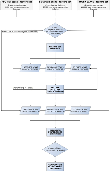
Figure 5. Workflow of multivariable analysis.
Download figure:
Standard image High-resolution image3. Results
3.1. Univariate results
Table 5 presents the Spearman's rank correlation (rs) between the nine non-texture features and lung metastases development in STSs. Table 6 presents the Spearman's rank correlation between the 205 different scan-texture features and lung metastases development in STSs. For each entry in table 6, two values appear: the rs in the case of texture features extracted using baseline parameters as defined in table 4 (left), and the maximal rs in the case of texture features extracted using the optimal set of extraction parameters when all parameters are allowed to vary, i.e. with full degrees of freedom (right). In tables 5 and 6, the values in italic font indicate features for which p < α/K < 0.05/(9 non-texture features + 5 scans × 41 textures × 2 extraction parameter degrees of freedom) ≈ 0.000 12 according to the correction for multiple testing comparison.
Table 5. Spearmans rank correlation (rs) between non-texture features and lung metastases development in STSs.
| Feature | rs | p-value |
|---|---|---|
| SUVmax | 0.52 | 0.0001 |
| Percent Inactive | 0.51 | 0.0001 |
| SUVpeak | 0.5 | 0.0002 |
| AUC-CSH | − 0.29 | 0.04 |
| Volume | 0.28 | 0.04 |
| SUVmean | 0.28 | 0.04 |
| Solidity | 0.24 | 0.09 |
| Size | 0.18 | 0.19 |
| Eccentricity | − 0.17 | 0.25 |
Note: The values in italic font indicate features for which p < 0.05/419 ≈ 0.000 12. AUC-CSH: Area under the curve of the cumulative SUV-volume histogram.
Table 6. Spearmans rank correlation between texture features and lung metastases development in STSs using baseline | optimal texture extraction parameters.
| Type | Texture | FDG-PET | T1 | T2FS | FDG-PET/T1 | FDG-PET/T2FS |
|---|---|---|---|---|---|---|
| Global | Variance | 0.12 | 0.13 | 0.21 | 0.21 | 0.03 | 0.05 | − 0.06 | −0.31 | − 0.44 | −0.49 |
| Skewness | 0.23 | 0.25 | − 0.36 | −0.36 | 0.16 | 0.17 | 0.13 | 0.28 | 0.28 | 0.39 | |
| Kurtosis | − 0.02 | 0.06 | − 0.28 | −0.31 | − 0.15 | −0.15 | − 0.11 | −0.24 | 0.33 | 0.42 | |
| GLCM | Energy | − 0.01 | 0.49 | − 0.22 | −0.44 | 0.14 | 0.23 | − 0.04 |  |
0.37 |  |
| Contrast | − 0.14 | −0.44 | − 0.08 | −0.33 | − 0.15 | 0.33 | − 0.19 |  |
− 0.36 |  |
|
| Entropy | 0.01 | −0.43 | 0.12 | 0.41 | − 0.15 | 0.22 | − 0.02 | −0.46 | − 0.38 |  |
|
| Homogeneity | 0.28 | 0.49 | 0.04 | 0.26 | 0.18 | 0.26 | 0.23 |  |
0.42 |  |
|
| Correlation | 0.28 | 0.42 | 0.18 | 0.32 | 0.15 | 0.25 | 0.26 | 0.42 | 0.10 | 0.38 | |
| Sum Average | − 0.35 |  |
0.28 |  |
− 0.11 | −0.29 | − 0.18 |  |
− 0.27 |  |
|
| Variance | 0.31 | −0.43 | 0.32 | 0.49 | − 0.07 | −0.26 | − 0.20 | −0.50 | − 0.32 |  |
|
| GLRLM | SRE | − 0.33 |  |
− 0.04 | −0.31 | − 0.18 | −0.34 | − 0.25 |  |
− 0.41 |  |
| LRE | 0.34 |  |
0.02 | 0.34 | 0.20 | 0.33 | 0.25 |  |
0.36 |  |
|
| GLN | 0.15 | 0.32 | 0.25 | 0.29 | 0.25 | 0.30 | 0.12 | 0.33 | 0.18 | 0.33 | |
| RLN | 0.13 | 0.32 | 0.26 | 0.30 | 0.22 | 0.30 | 0.14 | 0.33 | 0.14 | 0.33 | |
| RP | − 0.34 |  |
− 0.02 | −0.33 | − 0.19 | −0.34 | − 0.25 |  |
− 0.39 |  |
|
| LGRE | 0.29 | −0.48 | 0.06 | −0.37 | − 0.08 | −0.33 | 0.11 | −0.50 | − 0.16 |  |
|
| HGRE | − 0.23 | −0.32 | 0.23 | −0.47 | − 0.12 | −0.28 | − 0.12 | 0.48 | − 0.21 | 0.43 | |
| SRLGE | 0.26 | −0.49 | 0.08 | −0.44 | − 0.10 | −0.38 | 0.09 | −0.48 | − 0.17 |  |
|
| SRHGE | − 0.25 | −0.35 | 0.10 | −0.44 | − 0.17 | −0.31 | − 0.14 | −0.40 | − 0.25 | −0.44 | |
| LRLGE | 0.34 |  |
0.09 | 0.37 | 0.08 | 0.40 | 0.10 | 0.50 | − 0.11 |  |
|
| LRHGE | − 0.21 |  |
0.27 | 0.50 | 0.16 | 0.36 | − 0.11 |  |
− 0.12 |  |
|
| GLV | − 0.33 |  |
− 0.10 | −0.41 | − 0.28 | −0.39 | − 0.25 |  |
0.26 |  |
|
| RLV | − 0.31 |  |
− 0.18 | −0.38 | − 0.27 | −0.40 | − 0.27 |  |
− 0.35 |  |
|
| GLSZM | SZE | − 0.18 | −0.42 | − 0.05 |  |
− 0.05 | −0.35 | − 0.41 |  |
− 0.41 |  |
| LZE | 0.19 | 0.50 | 0.23 | 0.33 | 0.21 | 0.36 | 0.19 |  |
0.30 |  |
|
| GLN | 0.15 | 0.33 | 0.20 | 0.31 | 0.21 | 0.29 | 0.10 | 0.32 | 0.13 | 0.33 | |
| ZSN | 0.15 | 0.32 | 0.22 | 0.31 | 0.18 | 0.29 | 0.06 | 0.31 | 0.04 | 0.34 | |
| ZP | − 0.20 |  |
− 0.17 | −0.41 | − 0.15 | −0.34 | − 0.25 |  |
− 0.40 |  |
|
| LGZE | − 0.09 | −0.48 | 0.31 | 0.36 | − 0.01 | 0.36 | 0.12 | −0.46 | − 0.16 |  |
|
| HGZE | − 0.12 | 0.38 | − 0.19 | −0.40 | − 0.04 | −0.29 | − 0.17 | 0.50 | − 0.06 |  |
|
| SZLGE | − 0.22 | −0.46 | 0.28 | −0.39 | − 0.01 | 0.34 | 0.10 | −0.47 | − 0.19 |  |
|
| SZHGE | − 0.07 | 0.27 | − 0.17 | 0.47 | − 0.04 | 0.29 | − 0.31 |  |
− 0.21 | 0.50 | |
| LZLGE | 0.32 |  |
0.20 | 0.34 | 0.21 | 0.35 | 0.25 |  |
0.35 |  |
|
| LZHGE | 0.01 | 0.47 | 0.27 | 0.44 | 0.20 | 0.34 | 0.12 | 0.47 | 0.22 | 0.46 | |
| GLV | − 0.18 | −0.45 | − 0.25 | −0.34 | − 0.26 | −0.33 | − 0.21 |  |
− 0.24 |  |
|
| ZSV | − 0.21 | −0.48 | − 0.07 | −0.43 | − 0.05 | −0.33 | − 0.09 |  |
− 0.01 | −0.48 | |
| NGTDM | Coarseness | − 0.06 | −0.26 | − 0.22 | −0.28 | − 0.21 | −0.30 | − 0.08 | −0.29 | − 0.13 | −0.34 |
| Contrast | − 0.14 | −0.39 | 0.16 | 0.36 | 0.02 | 0.33 | − 0.11 | −0.46 | − 0.33 |  |
|
| Busyness | 0.23 | 0.39 | 0.22 | 0.28 | 0.22 | 0.30 | 0.20 | 0.39 | 0.17 | 0.39 | |
| Complexity | 0.21 |  |
− 0.16 | 0.39 | − 0.13 | 0.40 | 0.14 |  |
0.22 | −0.48 | |
| Strength | 0.04 | −0.25 | − 0.24 | −0.29 | − 0.21 | −0.29 | − 0.09 | −0.37 | − 0.07 | −0.33 | |
| Average absolute values | 0.20 | 0.42 | 0.18 | 0.37 | 0.15 | 0.31 | 0.16 | 0.46 | 0.24 | 0.49 | |
Note: The values in italic font indicate features for which p < 0.05/419 ≈ 0.000 12.
3.1.1. Non-texture features.
In table 5, it can be seen that the non-textural features that are highly correlated with lung metastases are SUVmax and Percent Inactive. Note the positive signs of rs for these two features.
3.1.2. Texture features.
In table 6, it can be seen that texture features extracted from FDG-PET scans generally have a higher predictive value than the texture features extracted from MRI scans. The results in table 6 also reveal that textures extracted from fused scans generally have a higher predictive value than those extracted from separate scans. Moreover, it can be seen that different extraction parameters significantly impact the predictive value of the resulting textures. The extraction parameters used to produce the texture features with the highest predictive value for the five different types of scans are presented in supplementary appendix B (stacks.iop.org/PMB/60/145471/mmedia).
3.1.3. Texture extraction parameter effect.
The Wilcoxon rank sum test was performed between the set of absolute Spearman's rank correlation coefficients obtained from each of the 41 different texture features extracted using baseline extraction parameters, and the sets of maximal absolute Spearman's rank correlation coefficients obtained from optimal texture-parameters for each of the 41 different textures when one extraction parameter was allowed to vary, and the others set to baseline. The same process was repeated for all parameters of all scans, and also for a Wilcoxon rank sum test comparing baseline extraction parameters to full degrees of freedom on extraction parameters (ALL PARAMs.). Table 7 presents the p-value of the Wilcoxon rank sum tests, with multiple testing corrections (α = 0.05, K = 29). The results point out that the optimization of the Scale texture extraction parameter has the highest impact on the predictive value for lung metastases development in STSs. In general, each extraction parameter seems to positively impact the predictive value of textures.
Table 7. p-value of the Wilcoxon rank sum tests asserting the significance of the effects of texture extraction parameters on the correlation of texture features with lung metastases development in STSs.
| Scan | MRI Inv. | MRI weight | WBPF | Scale | Quant. algo | Ng | ALL PARAMs. |
|---|---|---|---|---|---|---|---|
| FDG-PET | — | — | 0.0727 |  |
0.0017 | 0.0260 |  |
| T1 | — | — | 0.2406 |  |
0.1159 | 0.0369 |  |
| T2FS | — | — | 0.2105 | 0.0013 | 0.0066 | 0.0352 |  |
| FDG-PET/T1 | 0.1085 | 0.0019 | 0.0034 |  |
0.0024 | 0.0143 |  |
| FDG-PET/T2FS | 0.5937 | 0.1259 | 0.3076 | 0.0024 | 0.4143 | 0.3909 |  |
Note: The values in italic font indicate features for which p < 0.05/29 ≈ 0.0017. MRI Inv.: MRI Inversion, MRI weight: weight in FDG-PET/MRI fusion process, WBPF: wavelet band-pass filtering, Scale: isotropic voxel size, Quant. algo.: quantization algorithm, Ng: Number of gray-levels, ALL PARAMs.: all texture extraction parameters allowed to vary.
3.2. Multivariable results
We compared the prediction performance estimation of multivariable models constructed using three different types of initial feature sets: (i) FDG-PET textures + non-texture features; (ii) separate FDG-PET and MRI textures + non-texture features; and (iii) fused FDG-PET/MRI textures + non-texture features. We performed experiments for all degrees of freedom on texture extraction parameters. Figure 6 presents the prediction performance estimation of multivariable models with optimal degrees of freedom on texture extraction parameters, obtained separately for each model order of each initial feature set. Supplementary appendix C (stacks.iop.org/PMB/60/145471/mmedia) also provides detailed comparison between prediction estimates obtained in the experiments using baseline, full and optimal degrees of freedom on texture extraction parameters. Results show that multivariable models constructed with texture features extracted from separate scans provide no significant prediction estimation improvements as compared to multivariables models constructed with texture features extracted from FDG-PET scans only. On the other hand, multivariable models constructed from fused scans significantly improve the prediction performance estimation compared to FDG-PET scans alone.

Figure 6. Estimation of prediction performance of multivariable models constructed from FDG-PET scans, SEPARATE scans, and FUSED scans using optimal degrees of freedom on texture extraction parameters, for model orders of 1–10. The optimal degrees of freedom were found in terms of maximum 0.632+ bootstrap AUC, separately for each model order. Error bars represent the standard error of the mean on a 95% confidence interval.
Download figure:
Standard image High-resolution imageBy inspecting the curves in figure 6, we determined that the simplest multivariable model with best predictive properties (best parsimonious model) is obtained by linearly combining 4 texture features extracted from fused FDG-PET/MRI scans. The associated prediction performance estimation of this optimal combination of features using 1000 bootstrap samples yielded an AUC of 0.984 ± 0.002, a sensitivity of 0.955 ± 0.006 and a specificity of 0.926 ± 0.004. These last results were obtained using the 0.632+ bootstrap method, and as a comparison, the same model reached an AUC of 0.976 ± 0.002, a sensitivity of 0.938 ± 0.008 and a specificity of 0.892 ± 0.006 using the ordinary bootstrap method  . Next, the logistic regression coefficients of the final prediction model were computed using 1000 bootstrap samples. We hence propose the following complete multivariable model response g(xi) to be computed from fused FDG-PET/MRI scans at the time of diagnosis of STSs for the prediction of future lung metastases development:
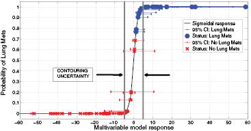
In order to evaluate the precision of the proposed model, we calculated how its response changes using texture features extracted from tumour contours that include surrounding edema. Supplementary appendix D.1 (stacks.iop.org/PMB/60/145471/mmedia) details the calculations. Overall, an absolute value of ± 4.89 was estimated as the uncertainty of the model due to contouring variations. This uncertainty is constant across all values of g(xi). Then, to summarize how the model can separate the instances of the two patient classes (LungMets versus NoLungMets), the vector  was computed for all patients using the multivariable model response of (7) and was transformed into the posterior probability π(xi) of observing outcome yi = 1 (i.e. developing lung metastases) given the input xi by using the logit transform of (2). Figure 7 displays the plot of π(xi) versus g(xi), along with the associated 95% confidence intervals (CIs) on g(xi) for i = 1, 2,..., N. For each bootstrap sample b used to calculate the final logistic regression coefficients of (7), a new value of
  was calculated for i = 1, 2,..., N from the new coefficients computed on
  . Then, the lower and upper CI bounds were estimated for each point i by calculating the 2.5 and 97.5 percentiles from the bootstrap distribution of
  for b = 1, 2, ..., B. In figure 7, the dots represent patients who eventually developed lung metastases, and the crosses those who did not develop lung metastases. The uncertainty due to contouring variations around the classification threshold g(xi) = 0 is also shown, and supplementary appendix D.2 (stacks.iop.org/PMB/60/145471/mmedia) provides the detailed data (lung mets status, g(xi) and CIs) used to construct the figure. It can be seen that the multivariable model of (7) can clearly separate the patients of the two risk groups. Note that the Spearman's rank correlation between the model response vector g and the outcome vector y reached rs = 0.84, p < 0.001.
Figure 7. Probability of developing lung metastases as a function of the response of the multivariable model proposed in this work, for all patients of the cohort.
Download figure:
Standard image High-resolution image
Finally, further validation of the proposed model was performed using permutation tests (Fisher 1935). This operation was carried out by randomly shuffling the real outcome vector y of our patient cohort (i.e. keeping the same proportion of 0's and 1's). In order to have a direct comparison with the model of (7), only the prediction performance of multivariable models of order 4 were analyzed. For each of the 1000 permutation tests, a different multivariable model was constructed and its prediction performance was assessed. Table 8 presents a summary of the results of the permutation tests, where the p-values were estimated using the Monte Carlo sampling approach described by Ernst (2004). Supplementary appendix E (stacks.iop.org/PMB/60/145471/mmedia) also provides a display of the permutation distributions. Overall, results in table 8 show that the null hypothesis can be rejected. Very few tests yielded prediction estimates higher than the true observed values. The results give strong evidence that the effect observed on the sample data is most likely present in the general STS population.
Table 8. Summary of permutation tests comparing the single value of the performance metrics estimates of the multivariable model proposed in this work found using the real outcome vector  to the distribution of the performance metrics estimates of models of order 4 found in 1000 permutation tests using shuffled outcome vectors
  . SD: Standard deviation.
| Metric |  |
 |
 |
 |
 |
 |
|---|---|---|---|---|---|---|
| AUC | 0.984 | 0.895 | 0.04 | [0.745, 0.988] | 3 out of 1000 | 0.004 |
| Sensitivity | 0.955 | 0.798 | 0.05 | [0.634, 0.938] | 0 out of 1000 | 0.001 |
| Specificity | 0.926 | 0.812 | 0.05 | [0.666, 0.948] | 6 out of 1000 | 0.007 |
4. Discussion
In this work, an imaging model was identified for the prediction of future lung metastases development at the time of diagnosis of STSs. This multivariable model is composed of four texture features extracted from fused FDG-PET/MRI scans. The use of texture features extracted from fused FDG-PET/MRI scans constitutes a new technique proposed in this work that revealed to be promising for tumour heterogeneity quantification. Our approach focused on standard-of-care medical images in order to strengthen its clinical impact. We believe that the methodology developed in this work could be generalized to other types of cancer and tumour outcomes.
First, the association of nine non-texture features with lung metastases development in STSs was presented in table 5. As expected, SUVmax was significantly associated with lung metastasis risk in STS cancer, a result in agreement with other studies (Schwarzbach et al 2000, Eary et al 2002, Skamene et al 2014). A significant positive association was also found between Percent Inactive and lung metastases development, meaning that the larger the volume of inactive FDG-PET regions in reference to patient-specific SUVmax values, the higher the risk of developing lung metastases in STS cancer. In table 6, the strong and positive associations of Homogeneity and LZE, and the strong and negative association of Complexity, for example, corroborate this last assertion. This could be explained from the fact that patients from the LungMets group often possess large and uniform low-uptake regions (as compared to maximum SUV) in the inner portion of their tumour on FDG-PET scans, most likely representing necrotic areas. The presence of these inner, low-uptake uniform regions suggests that the tumour is rapidly increasing in size and might be more at risk to metastasize. As demonstrated, texture analysis can however reveal more information about the tumour underlying biology than simple imaging metrics: for example, the strong and positive association of the LZLGE metric with lung metastases confirms that large low-uptake regions in FDG-PET have significant predictive value, but the positive association of the LZHGE metric (although to a lesser extent) suggest that large high-uptake regions may also play an important role in the characterization of aggressive tumours. Note that this last information would not have been captured by textures extracted with standard baseline parameters (defined in table 4) only. This suggests that texture optimization is a desirable property to enhance the predictive value of textures, and table 7 revealed that Scale is the extraction parameter that has the most influence on texture definition. An image with a given intrinsic resolution but resampled to different resolutions will produce different texture measurements, as imaging patterns are better captured for a certain range of resolutions. In this sense, an optimal scale at which textures offer best discrimination between the two classes of STS patients likely exists. In general, different texture features will better represent the underlying tumour biology using different extraction parameters, and the optimal set of parameters to use is application-specific and will depend on many factors such as the clinical endpoint studied and the imaging modalities employed.
Furthermore, the results presented in figure 6 showed that MRI textures alone are generally not useful in comparison to FDG-PET textures. However, the addition of the MR imaging information to FDG-PET in the fusion process seems to significantly improve and even stabilize the prediction performance estimation of FDG-PET textures. Although some information may be lost in the fusion process, the fusion of FDG-PET and MRI scans may create new textural properties that can better characterize intratumoural heterogeneity than what separate FDG-PET and MRI scans can provide. Figure 7 then illustrated how the prediction model proposed in this work could be clinically used for the evaluation of the risk of future lung metastases development in STSs. A patient diagnosed with STS cancer would present in a hospital and undergo FDG-PET and MRI scans (with both T1 and T2FS sequences). A single value of the form of (7) could then be obtained by extracting specific textures features from fused FDG-PET/MRI scans. Using the logit transform of (2), this value could be transformed into the probability of developing lung metastases. This probability could then provide useful insights to physicians into risk assessment and treatment personalization. Ultimately, provided a given decision threshold and confidence interval, standard treatments could be strengthened for high risk patients and lessened for low risk patients. However, it can be seen from figure 7 that the statistical uncertainty on g(xi) measurements (bootstrap CIs) inherent to logistic regression coefficient estimates is significant and constitutes the principal limiting factor of the proposed model. A larger patient cohort is first needed to improve its precision. Moreover, a constant uncertainty of ± 4.89 on g(xi) measurements due to contouring variations was found. This uncertainty on g(xi) = 0 incorporates 19 patients of our cohort (9 from the LungMets group, 10 from the NoLungMets group), and no definitive conclusion could be drawn for these patients in a clinical decision-support system. This emphasizes the need to identify a model that can yet better separate the two patient classes, but also to construct texture-based prediction models from tumours delineated using automatic segmentation methods.
Overall, the multivariable model proposed in this work was found to possess high predictive potential for lung metastases in STS cancer. However, a larger patient cohort is needed to create a more robust model, and independent testing on external datasets is required to confirm its predictive properties. Once this step is cleared, we should investigate how this texture-based model could complement clinical prognostic factors for optimal prediction. The extraction of texture features from medical images and the construction of prediction models are complex processes that need proper validation, and much effort is still required in order to achieve clinical implementation of a texture-based decision-support system. First, a consensus on techniques used for imaging acquisition, data pre-processing, tumour delineation, texture analysis and multivariable modeling is needed in the radiomics community. Assuredly, standardization and full transparency on data and methods is the key for the progression of the field (Lambin et al 2013).
5. Conclusion
Textural biomarkers as an intratumoural heterogeneity quantification tool hold great promise for the early prediction of tumour outcomes. In this work, we explored a novel approach based on the fusion of FDG-PET and MRI volumes to better quantify intratumoural heterogeneity using texture analysis. Innovative texture extraction techniques and multivariable modeling strategies were also developed for the construction of tumour outcome prediction models from a large number of radiomics features. The results showed that FDG-PET and MRI texture features could act as strong prognostic factors of STSs and could provide insights about their underlying biology. FDG-PET texture features were shown to generally possess a higher predictive value than MRI texture features for lung metastases in STS cancer, but their predictive value was significantly enhanced by the addition of the MR imaging information to FDG-PET via the fusion process. The results also pointed out the importance of the optimization of texture extraction parameters to enhance their predictive value and to better understand the relation between textures and biology. Ultimately, we identified a model combining four texture features extracted from fused FDG-PET/MRI pre-treatment scans to predict future lung metastases development in STSs. This model reached high prediction performance estimates in bootstrapping evaluations and was validated using permutation tests. However, further validation on independent datasets is required to confirm its predictive properties. We believe that the methodology presented in this work could be generalized to other types of cancers and that it could eventually lead to improvements in treatment personalization and patient survival.
Online resources
Clinical information and imaging data analyzed in this work are available on The Cancer Imaging Archive (TCIA) website under the following DOI: http://dx.doi.org/10.7937/K9/TCIA.2015.7GO2GSKS. All software code implemented in this work is freely shared under the GNU General Public License at: https://github.com/mvallieres/radiomics.
Acknowledgments
This work was supported by the Natural Sciences and Engineering Research Council (NSERC) of Canada under the scholarship CGSD3-426742-2012, as well as it was partly supported by the Canadian Institutes of Health Research (CIHR) under grants MOP-114910 and MOP-136774, and the NSERC of Canada under the grant RGPIN 397711-11.