
Abstract
Previous studies have shown that during cancer radiotherapy a small translation or rotation of the tumor can lead to errors in dose delivery. Current best practice in radiotherapy accounts for tumor translations, but is unable to address rotation due to a lack of a reliable real-time estimate. We have developed a method based on the iterative closest point (ICP) algorithm that can compute rotation from kilovoltage x-ray images acquired during radiation treatment delivery. A total of 11 748 kilovoltage (kV) images acquired from ten patients (one fraction for each patient) were used to evaluate our tumor rotation algorithm. For each kV image, the three dimensional coordinates of three fiducial markers inside the prostate were calculated. The three dimensional coordinates were used as input to the ICP algorithm to calculate the real-time tumor rotation and translation around three axes. The results show that the root mean square error was improved for real-time calculation of tumor displacement from a mean of 0.97 mm with the stand alone translation to a mean of 0.16 mm by adding real-time rotation and translation displacement with the ICP algorithm. The standard deviation (SD) of rotation for the ten patients was 2.3°, 0.89° and 0.72° for rotation around the right–left (RL), anterior–posterior (AP) and superior–inferior (SI) directions respectively. The correlation between all six degrees of freedom showed that the highest correlation belonged to the AP and SI translation with a correlation of 0.67. The second highest correlation in our study was between the rotation around RL and rotation around AP, with a correlation of −0.33. Our real-time algorithm for calculation of rotation also confirms previous studies that have shown the maximum SD belongs to AP translation and rotation around RL. ICP is a reliable and fast algorithm for estimating real-time tumor rotation which could create a pathway to investigational clinical treatment studies requiring real-time measurement and adaptation to tumor rotation.
Export citation and abstract BibTeX RIS

Content from this work may be used under the terms of the Creative Commons Attribution 3.0 licence. Any further distribution of this work must maintain attribution to the author(s) and the title of the work, journal citation and DOI.
General scientific summary Measuring the motion of tumors in real-time during cancer radiotherapy is the subject of intense research and clinical translation. To date, research has focused on translational motion. However, tumors also rotate during cancer radiotherapy and measuring and correcting for rotation will enable better cancer targeting. This paper describes a new method to measure tumor translation and rotation during cancer radiotherapy using the kilovoltage imager. We extended our existing method that converts two-dimensional kilovoltage image information into three dimensional motion by invoking an iterative closest point algorithm to obtain six degrees-of-freedom translation and rotational motion. The method was tested on images acquired from ten prostate cancer patients during radiotherapy resulting in realistic real-time translation and rotation estimates. Given that kilovoltage imagers are available on most new cancer radiotherapy systems, this method has the potential for widespread implementation for more accurate radiotherapy for thoracic, abdominal and pelvic cancer patients. For more information on this article, see medicalphysicsweb.org
1. Introduction
Image guided radiotherapy (IGRT) using onboard kilovoltage imagers is an effective localization method to reduce the uncertainties in the estimation of tumor location and aids in patient positioning (Dawson and Jaffray 2007). IGRT has also been used for monitoring the target in real-time during radiation delivery (Poulsen et al 2008b, 2010b, Ng et al 2012). As it is difficult for the 2D kilovoltage (kV) imaging system to image soft tissue, oncologists implant radiopaque markers in the vicinity of the tumor and use the markers as indicators to determine the location of the tumor (Vigneault et al 1997). Although IGRT is used extensively to position patients for radiotherapy treatment, tumor rotation is not currently considered during the treatment planning and delivery of radiotherapy.
For real-time estimation of prostate tumor location, two uncertainties need to be considered: setup related errors and organ or tumor motion, which contain both a systematic and random component (Remeijer et al 2000, Bel et al 1996, van Herk et al 1995, Rasch et al 1993). Nichol et al (2007) found that the standard deviations (SDs) of systematic and random uncertainties caused by prostate deformation were 0.8 mm and 1.5 mm respectively. Separating the systematic and random errors is important because each error type has a different effect on the dose distribution. Random errors blur the dose distribution, while systematic errors cause a shift of the cumulative dose distribution relative to the target (Lujan et al 1999, Leong 1987).
In addition to prostate tumor translation, prostate tumor rotation during treatment can also affect the target dose coverage. For that reason, a small rotation may cause some part of the tumor to receive a dose that is lower than the prescribed amount. Previous studies on prostate rotation show that rotational errors are significant in some cases (Remeijer et al 2000, van Herk et al 1995). Van Herk et al (1995) reported that prostate rotation is small, except for rotation around the right–left (RL) axis (4.0°). Li et al (2009) established a relationship between prostate tumor rotation and the efficacy of radiation treatment. They found an average margin reduction from 6.2 to 4.9 mm when rotational correction was added to a 4D adaptive treatment and conclude 'prostate intrafractional motion control and rotation correction may improve treatment for this group of (prostate) patients and the overall clinical outcome will be improved'. Deutschmann et al (2011) developed and evaluated a correction strategy for prostate rotations (but not in real-time) using direct adaptation of segments in intensity-modulated radiotherapy (IMRT). Their results showed that rotation around RL is up to 5.3° (mean of means), with a SD of ±4.9°. Graf et al (2012) reported the interfraction rotation errors of the prostate around the three axes anterior–posterior (AP), superior–inferior (SI), and RL (0.09°, −0.52° and −0.01°) with SD s of 2.01°, 2.30° and 3.95°, respectively. They estimated systematic uncertainty per patient for prostate rotation with 2.30°, 1.56° and 4.13° and the mean random components with 1.81°, 2.02° and 3.09°. They also reported that the largest rotational errors occurred around the RL axis, but without preferring a certain orientation. There have been several studies to correct for tumor rotation and to reduce treatment margins for IMRT (Hoogeman et al 2005, van Herten et al 2008, Krauss et al 2011, Sawant et al 2008). These studies have corrected for rotation by moving or rotating the gantry, collimator, and/or couch in real-time or by using a dynamic multi leaf collimator. Wu et al (2012) demonstrated the ability to correct for in-plane target rotation using a research version of the Calypso system integrated with a real-time DMLC tracking system.
The current study estimates real-time rotation from x-ray images acquired during radiotherapy by extending Poulsen's (Poulsen et al 2008b) translation estimation method via an iterative closest point (ICP) algorithm.
2. Material and methods
2.1. Coordinate systems and the iterative closest point algorithm
There are many ways to represent rotation, such as: Euler angles, Gibbs vector, Cayley–Klein parameters, Pauli spin matrices, axis and angle, orthonormal matrices and Hamilton's quaternions (Korn and Korn 1968, Stuelpnagle 1964). In this study, Euler angles were used as it is more convenient for real-time tracking on a linac system; rotational variations about the RL, SI and AP axes are the Euler angles θRL, θSI and θAP, respectively.
The estimation of rotation matrix and translation vector parameters (also called pose estimation) is a common problem in computer vision. One of the first studies was by Thompson (1958) who developed a method that calculates rotation when three data points are available. The method of Thompson (1958) depends on selective neglect of the extra constraints when all coordinates of three points are known. Schut (1960) proposed an alternative method based on unit quaternion and a set of linear equations. However, neither method handles more than three data points nor they use all the information available from the three points. More recently, Arun et al (1987) developed a numerical least squares fitting method using only two data points. Their algorithm was based on the singular value decomposition (SVD) of a 3 × 3 matrix. A closed form solution to the least squares problem for three or more points was developed by Horn (1987). Deriving the solution was simplified by using unit quaternion to represent rotation. However, due to reflection, the Arun and Horn methods fail to determine the correct rotation matrix when the data is extremely noisy. These problems with reflection were addressed by Umeyama (1991) by changing the matrix of the solution.
In this study, we implemented the Umeyama method and the ICP algorithm (figure 1) to estimate rotation and also examine the maximum error level according to this estimation (Chen and Medioni 1991). Figure 1 shows the steps for the ICP algorithm in more detail.
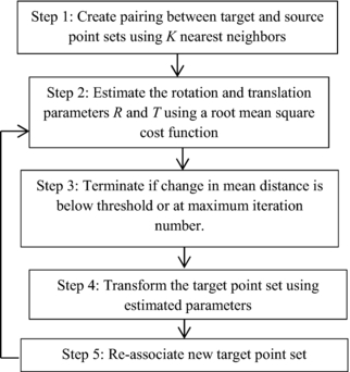
Figure 1. Block diagram for estimation of rotation using ICP algorithm with fiducial markers.
Download figure:
Standard image High-resolution image2.2. Image acquisition
A total of 11 748 images acquired during one fraction of the treatment of ten prostate cancer patients with radiopaque prostate markers were used in this study (Ng et al 2012). Images during VMAT treatment were acquired by a kV x-ray imager mounted perpendicularly to the radiation treatment beam source (OBI, Varian Medical Systems). All treatments were dual-arc VMAT with similar treatment times and the number of images per patient was similar. The exposure parameters used were 125 kVp, 80 mA and 13 ms (a standard pelvic cone beam computed tomography scan setting) with a 6 × 6 cm2 field size (no filter was used). The imaging frequency was 5 or 10 Hz, depending on the desired image quality. During treatment, to reduce scatter from the MV source, the kV source to detector distance was set to 180 cm (compared with 150 cm for CBCT). The estimated imaging dose for kilovoltage intrafraction imaging is 185 mGy over the course of a conventionally fractionated prostate IMRT treatment. More details of the dose estimates are given in Crocker et al (2012).
2.3. Pose estimation of fiducial markers
As the gantry rotates around the patient during treatment, two dimensional projections of the prostate are acquired at time tk by a kV imager. The fiducial markers are segmented and extracted using in-house software (Fledelius et al 2011b). Figure 2 is a screenshot showing a kV image with three radiopaque markers and the segmented location of the markers as determined by our in-house software.
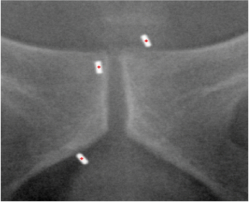
Figure 2. Two dimensional kV imaging of three gold radio opaque fiducial markers implanted in the prostate of a patient. The red dots indicate the location of the marker as segmented by our in-house software.
Download figure:
Standard image High-resolution imageTo determine the three dimensional location of the markers from a series of two dimensional segmented markers, a three dimensional Gaussian probability distribution function (PDF) is assumed for each marker (Poulsen et al 2008b). The influence of the PDF does not affect the comparison because in both methods (three dimensional and ICP algorithm) the calculation of the PDF is the same. However, the use of the PDF itself (and errors in marker segmentation) may induce uncertainty in the rotation estimation. The covariance matrix and mean marker location used by the PDF are determined by fitting the PDF to a series of two dimensional marker locations by the maximum likelihood estimation. The three dimensional locations of the markers are determined from the three dimensional PDF using the method of Poulsen et al (2008a).
2.4. Estimation of rotation and translation
Let us assume that we have two sets of data points for the fiducial markers, a source point at time t1 and a target point at time tk. The source points are determined during a pretreatment arc that is necessary to build the PDF needed for the translation (and rotation) estimation prior to turning the treatment beam on (Ng et al 2012). The target point at time tk is obtained by rotating the source point, t1, around an axis and/or translating, the source point t1, along an axis with an unknown transform function. As implemented the rotation matrix of the ICP algorithm is computed about the center of mass of the markers after the shift of the translation T. The set of source points, one for each marker, are denoted by Q = (q1, q2, ..., qN) and the set of target points, one for each marker, are denoted by P = (p1, p2, ..., pN), where N is the number of fiducial markers. We assume that all markers are translated and rotated by the same amount, so that

where R is the rotation matrix, T is the translation vector, s is the scaling factor and n is the noise (assuming the noise is Gaussian). We separate the rotation matrix into its components about each axis:


The ICP algorithm iteratively performs matching for every data point based on the nearest neighbor algorithm (Cover and Hart 1967), see step 1 in figure 1. In our context, this step is not normally needed because it is easy to identify which marker the data point belongs to. The nearest neighbor analysis is very important when two or more of the fiducial markers are close to each other and could be mistakenly identified. The three fiducial markers in most of the data studied in this research were placed sufficiently far apart to avoid mismatching. In clinical practice, either sufficient marker separation would be required or robust methods to account for the issues with overlapping markers would need to be developed.
For step 2 in figure 1, we plan to estimate the rotation and transformation matrices, R and T. To do this, we minimize the sum of the squared distances of target to source points (Besl and McKay 1992). This forms the error function f(R, T) ≈ n (n is the noise in equation (1)) that we wish to minimize and is mathematically expressed as

We estimate R and T using SVD (Umeyama 1991) which is described in more detail in the appendix. Note that in equation (6) we have set the scale factor, s, to 1. The scale factor will be calculated based on the area of triangles after calculating rotation and translation. The scale factor is essentially the relative area of the triangle made by the three markers. A variation in the scale could indicate errors in marker segmentation or indicate prostate deformation. During an individual fraction marker segmentation errors are more likely than prostate deformation, so we can use the scale factor as a threshold to remove suspected marker segmentation errors.
Using our estimates of R and T, we iteratively update the values using the following algorithm (step 3–5 in figure 1). We use two intermediate matrices, Rit which we initially set to the 3×3 identity matrix, and Tit which we initially set to the 3×1 zero vector. These two matrices are updated according to


where k is the iteration number; in this case we terminate after a maximum of five iterations. In step 4 of figure 1, the new point Pk + 1 is calculated from the new update of the following equation:

where repmat (Tit(k + 1)1, 3) is a matrix consisting of a 3 × 1 tiling of copies of Tit(k + 1). Now that we have a new value for Pk + 1, we calculate new estimates for R and T using equation (6), i.e. the new estimates, Rk + 1, and Tk + 1 are found with
Convergence usually occurs in fewer than 5 iterations (see figure 3 for an example of the error for 21 iterations). In our implementation we perform at most five iterations and the final value of Pk + 1 is used to estimate the root mean square error (RMSE) of the matrix transformation using equation (10)

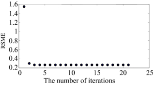
Figure 3. An example of the iterative curves for calculating the rotation matrix using ICP. The number of iterations is 21 in this example, with convergence occurring after 3 or 4 iterations.
Download figure:
Standard image High-resolution imageThe final step is to calculate the Euler angles, θRL, θSI, θAP, from the rotation matrix, R, using a nonlinear least square fitting algorithm (Klumpp 1976, Weisstein 2013) for the new fiducial marker positions.
A program has been written in C# to show the 3D trajectory of the markers as calculated in Poulsen et al (2008b) with the addition of the rotation calculations as presented in this study. Figure 4 shows the main screen of the software which shows, in real-time, the latest kilovoltage image with the segmented 2D marker locations, a graphical view of the markers in the middle, the 3D trajectory of the markers and the rotation of the markers.

Figure 4. The main screen of the fiducial marker tracking application. In the top left is the latest kilovoltage image showing the segmented marker locations. In the middle is a three dimensional view of the markers. In the bottom left the value of the rotation around RL (blue), rotation around SI (yellow), and rotation around AP (red) in degrees are shown. In the bottom right trajectory of the markers in RL (blue), SI (yellow), AP (red) are shown. A movie of this application is included as supplemental material stacks.iop.org/PMB/58/8517/mmedia.
Download figure:
Standard image High-resolution image3. Results
We started our analysis of the algorithm using an example where we knew the rotation of the markers. We analyzed the performance of the algorithm for prostate cancer patients later in this section.
3.1. Rotation results from ground truth data
In order to evaluate the method, we simulated the rotation of three fiducial markers based on assuming the 3D positions were perfectly estimated. In each simulated image, the triangle formed by the three fiducial markers was rotated in each subsequent image by θRL = 0.1°, θSI = 0.2°, θAP = 0.3°. Figure 5 shows the value of the rotation around RL, rotation around SI and rotation around AP sequentially.
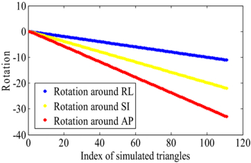
Figure 5. The rotation as computed from the ICP algorithm for a simulated scenario. The three fiducial markers forming a triangle were rotated by (θRL = 0.1°, θSI = 0.2°, θAP = 0.3°) in each subsequent image.
Download figure:
Standard image High-resolution imageThe mean of the RMSE between the source points and transformed target points (equation (10)) were calculated up to 30°. Figure 5 shows the linear incremental rotation of up to 30° for three directions. The maximum error up to 30° was 0.007° with a mean value of 0.004°. Rotations of 30° are above the rotations that we observed in the next section for prostate cancer patients.
3.2. Prostate cancer rotation results from clinical intrafraction x-ray images
In this section, we extended our analysis to prostate cancer patients where we calculated the real-time prostate rotation and translation of the prostate for ten prostate cancer patients. In figures 6(a) and (b) an example of the time series of rotation and translation is illustrated for a prostate cancer patient. Rotations of over 7° are observed for this patient. The translation and rotation data are relatively noisy because of the noisy data in the 2D segmented location of the markers. However, a clear trend in the rotation data is visible in figure 6(a).
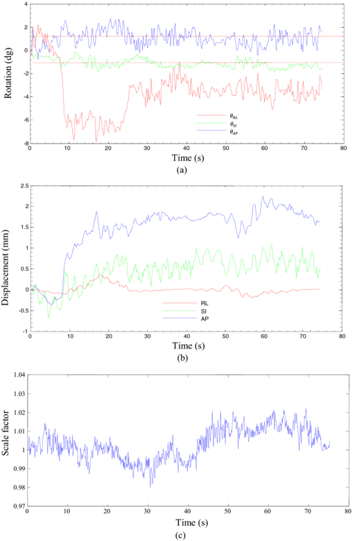
Figure 6. (a) An example of prostate rotation angles computed from intrafraction kV images using the ICP algorithm for a prostate cancer patient. The dashed line shows threshold for 1° rotation. (b) An example of prostate translation for the same prostate cancer patient, and (c) a typical curve of normalized scale factor related to the rigidity of the tumor.
Download figure:
Standard image High-resolution imageFigure 6(c) shows variations in the scale factor, s, for the same patient. The scale factor was calculated based on the changes in the area of the triangles formed by the three fiducial markers relative to the area of the triangle in the first image. Figure 7 gives a graphical view of the triangle formed by the markers. Figure 8 shows the variation of the scale factor for the whole dataset (11 748 images). The correlation coefficient of the template based marker segmentation (Fledelius et al 2011b) and scale factors were implemented to detect and remove noise in the rotation calculations. In this study, the threshold for correlation was 0.65 and the threshold for the scale factor set for values with more than a 5% change in size (1 ± 0.05). Less than 2% of the data were removed based on these thresholds. Figure 9 shows the histogram of the translation and rotation parameters. For rotation, the center of θRL was around 1°, while θSI and θAP were centered around 0°. For translation, the SI and RL histograms are centered close to 0 mm, while the center of the AP histogram is around 0.3–0.4 mm. Figure 10 shows the pair-to-pair datapoints and the correlation of the variables to each other in the upper right hand triangle. The maximum correlation was between SI and AP translations with a correlation coefficient of 0.66. This is consistent with the results from Poulsen et al (2008b). The correlations between θRL, θSI and θAP also had values higher than 0.1 with a negative correlation between θRL and θAP. Figure 10 also shows that the correlation between θSI and θAP was almost two times larger than correlation between θRL and θSI.

Figure 7. The vertices of the triangle formed by the three fiducial marker locations inside the prostate over time. The scale factor, s is calculated based on the change in the area of the triangles.
Download figure:
Standard image High-resolution image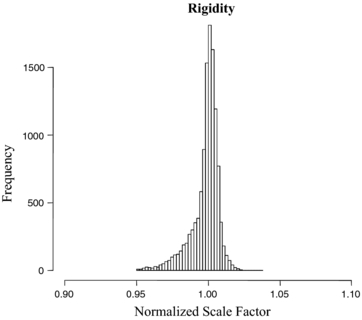
Figure 8. Number of occurrences of the scale factor, s, of the triangles for the 11 748 images acquired from ten prostate cancer patients.
Download figure:
Standard image High-resolution image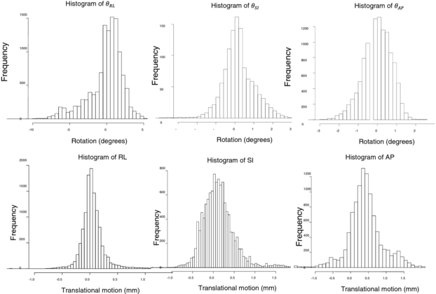
Figure 9. Histograms of rotation and translation of the fiducial markers.
Download figure:
Standard image High-resolution image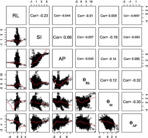
Figure 10. Correlation between translations and rotations for 11 748 images. The red lines are the nonlinear curve fitting using lsqcurvefit (Matlab function) to the data.
Download figure:
Standard image High-resolution imageIn table 1 the value of SD of rotation and translation is given in millimeters and degrees, respectively. The maximum value of SD is θRL with 2.3° of rotation.
Table 1. Standard deviation of rotation and translation.
 |
 |
 |
RL (mm) | SI (mm) | AP (mm) |
|---|---|---|---|---|---|
| 2.26 | 0.89 | 0.72 | 0.32 | 0.53 | 1.13 |
Figure 11 shows the RMSE values between the source points and transformed target points (equation (10)) of the rotation with the ICP and translation only. The x-axes show the distance error of the transformed points using the new rotation matrix R and translation vector T. The mean, median and SD of the errors is given in table 2. The ICP algorithm had a sub-0.2 mm mean, median and SD. These values were significantly smaller compared to those of the translation only algorithm.

Figure 11. (Top) RMSE values of translation and rotation with ICP after 20 iterations of the ICP algorithm. (Bottom) RMSE values of translation only.
Download figure:
Standard image High-resolution image
Table 2. Mean and standard deviation of iterative closest point (ICP) and translation only.
| Mean | SD | Median | |
|---|---|---|---|
| Error with ICP | 0.16 mm | 0.11 mm | 0.12 mm |
| Error with translation | 0.97 mm | 0.94 mm | 0.66 mm |
4. Discussion
In this study, the ICP algorithm was evaluated for real-time estimation of rotation during external beam radiation treatment. Real-time rotation was estimated from three fiducial markers located inside the prostate. The results show that the ICP algorithm converged after two or three iterations to the minimum value. The RMSE deviation of the ICP algorithm was compared with the RMSE error of the displacement using standalone translation and the result showed significant improvement. The additional computation of rotation only adds a few milliseconds to the time used for marker segmentation and 3D position estimation, which is approximately 30 ms (Poulsen et al 2010a). Therefore we would expect the total latency of a real-time clinical rotation estimation system to be less than 300 ms, similar to that measured in end-to-end experiments of kV-image based translation tracking (Fledelius et al 2011a).
Table 3 shows the summary of previous studies of prostate rotation using electromagnetic tracking compared with the current findings. The smaller rotation values reported in our study compared to those of Li and Olsen using electromagnetic tracking are likely due to a difference in the reference pose, or simply different patients.
Table 3. A comparison of previous electromagnetic tracking tumor rotational measurements of the prostate with the kV imaging/ICP algorithm results.
| Rotation mean ± std dev (°) | ||||||
|---|---|---|---|---|---|---|
| Study author | Number of patients | Measurement method | Comments | RL (Pitch) | SI (Roll) | AP (Yaw) |
| Olsen et al | 15 | Electromagnetic | Reference pose | 5.7 ± 5 | 2.0 ± 2 | 1.6 ± 1 |
| (2012) | tracking | from CT simulation | ||||
| Li et al | 29 | Electromagnetic | Reference pose from | 1.5 ± 5.2 | 0.4 ± 1.7 | 0.8 ± 1.6 |
| (2009) | tracking | first treatment fraction | ||||
| This work | 10 | kV imaging with | Reference pose from | 0.1 ± 2.3 | 0.2 ± 0.9 | −0.01 ± 0.7 |
| the ICP algorithm | first image in each | |||||
| treatment fraction | ||||||
The correlation and covariance of rotation and translation were calculated. The covariance of rotation and translation was smaller than the values were published by Poulsen et al (2008b) who used 1 min traces. However, the correlations between parameters were similar in this study to the correlation values in Poulsen's study. The reason for these differences was that we were calculating the error of transformation for small motions of the prostate by using two thresholds: one on the correlation between measured data (cor = 0.65) and the other on scale factor (sf = 1 ± 0.05). The calculated error for ICP was 0.166 mm. Some part of this error was expected because of the three dimensional PDF function we used for calculating the three dimensional translations. However, increasing the number of fiducial markers could reduce the value of the RMS error. At present, three fiducial markers are typically implanted in clinical prostate treatments. One of the future directions for this study could be a study of the RMS error for three to five fiducial markers on a phantom to investigate whether the residual error can be further reduced. We also suggest further study on a phantom and a large clinical data set to improve the three dimensional Gaussian PDF to a six dimensional PDF. An additional step required for a clinical implementation would be to use the marker positions from the planning CT scan as the source points rather than those from the pretreatment arc. This would enable the absolute rotational pose from the plan to be computed.
For transforming the rotation matrix to Euler angles, the order of rotation around the axes was selected as RL, SI, and AP respectively. The reason for this choice is that the Euler angles are more understandable from a clinical perspective than other choices such as unit quaternions (Horn 1987). The order of rotation around the axes could affect the final value of rotation. However, in this study, the rotation of prostate was mostly less than 10° with RL having the dominant rotation. The order in which we select rotation around the axes has little effect. For larger rotations, the choice of the order of rotation needs to be studied.
A sensitivity analysis of the effect of marker segmentation error and the impact of the use of the PDF to generate the 3D translation values will form the basis of further work using a larger clinical dataset. From the current results (figure 6) it appears the marker segmentation adds approximately 1° of noise to the rotational estimates. This noise could be reduced through improved marker segmentation algorithms and/or signal processing methods such as trend filtering and incorporating mechanical constraints based on known maximum organ translation and rotation.
There are several natural extensions of the current framework to be explored.
- (1)As the scale factors of the triangles formed by the markers are computed as part of the ICP algorithm, some estimate of target deformation may be possible, or this information used as a warning indicator for potential changes during treatment.
- (2)The algorithm currently ignores information from the megavoltage (MV) beam. Even for modulated beams some of the markers may be visible for some of the time. The use of the MV information could be used to augment the kV information. Alternatively, in some situations the ICP method could be implemented with the MV beam alone.
- (3)A disadvantage of kV intrafraction monitoring is the increased x-ray imaging dose. To reduce the dose, for tumor sites with a respiratory motion component, the kV information could be augmented by a respiratory signal through an internal–external model, e.g. by an extension of the Cho method to include rotation (Cho et al 2012).
5. Conclusion
A method of real-time estimation of prostate tumor rotation and translation (6D) using a single imager kilovoltage intrafraction monitoring has been developed.
The estimation method has been applied to a ten-patient dataset. Given the widespread availability of cancer radiotherapy systems with single x-ray imagers, this method could have a major impact on prostate IGRT accuracy and potentially other tumor sites where three or more implanted markers are routinely placed.
Acknowledgments
Professor PK acknowledges the financial support of an NHMRC Australia Fellowship. Jin Aun Ng, Jeremy Booth, Thomas Eade, Andrew Kneebone and Walther Fledelius are acknowledged for their work on the clinical implementation of the kilovoltage intrafraction monitoring program, and Dr Chen-Yu Huang for contributions quantifying target rotation. Julie Baz reviewed and improved the clarity of the paper.
: Appendix
The following describes the method for calculating the rotation matrix, R, and the translation vector T. Let qi and pi for i = 1, 2, .., N denote the location of the N fiducial markers in time t1, and tk, respectively. The centroid of the system of markers is


The deviations from the centroid are given by

The translation vector T should be chosen to move the centroid of the target dataset to the centroid of the source dataset:

Substituting the equations for and
and  in equation (6) and after some simplification we have

where the trace of a matrix A is the sum of the diagonal elements of A:tr(A) =  For convenience we set
 ![$M = \mathop \sum \nolimits_{i = 1}^N p_i ^\prime q_i ^{\prime^{T}} = [ {c_1 ,c_2 , \ldots ,c_N }],$](https://content.cld.iop.org/journals/0031-9155/58/23/8517/revision1/pmb484778ieqn9.gif) and R = [r1, r2, ..., rN] where ci and ri are the column vectors of M and R respectively. We maximize the trace tr(MRN) in order to minimize f(R, T):
and R = [r1, r2, ..., rN] where ci and ri are the column vectors of M and R respectively. We maximize the trace tr(MRN) in order to minimize f(R, T):

Since the rotation matrix R is orthogonal by definition, its row vectors all have unit length. This inequality is a reformulation of the Cauchy–Schwarz inequality (Buskes and van Rooij 2000)

The SDV of  ensures that the algorithm always provides the rotation matrix and not the reflection matrix. Finally, R can be calculated using

where diag is the diagonal matrix and det is the determinant of the matrix.