
Abstract
High intensity focused ultrasound (HIFU) enables highly localized, non-invasive tissue ablation and its efficacy has been demonstrated in the treatment of a range of cancers, including those of the kidney, prostate and breast. HIFU offers the ability to treat deep-seated tumours locally, and potentially bears fewer side effects than more invasive treatment modalities such as resection, chemotherapy and ionizing radiation. There remains however a number of significant challenges which currently hinder its widespread clinical application. One of these challenges is the need to transmit sufficient energy through the ribcage to ablate tissue at the required foci whilst minimizing the formation of side lobes and sparing healthy tissue. Ribs both absorb and reflect ultrasound strongly. This sometimes results in overheating of bone and overlying tissue during treatment, leading to skin burns. Successful treatment of a patient with tumours in the upper abdomen therefore requires a thorough understanding of the way acoustic and thermal energy is deposited. Previously, a boundary element approach based on a Generalized Minimal Residual (GMRES) implementation of the Burton–Miller formulation was developed to predict the field of a multi-element HIFU array scattered by human ribs, the topology of which was obtained from CT scan data (Gélat et al 2011 Phys. Med. Biol. 56 5553–81). The present paper describes the reformulation of the boundary element equations as a least-squares minimization problem with nonlinear constraints. The methodology has subsequently been tested at an excitation frequency of 1 MHz on a spherical multi-element array in the presence of ribs. A single array–rib geometry was investigated on which a 50% reduction in the maximum acoustic pressure magnitude on the surface of the ribs was achieved with only a 4% reduction in the peak focal pressure compared to the spherical focusing case. This method was then compared with a binarized apodization approach based on ray tracing and against the decomposition of the time-reversal operator (DORT). In both cases, the constrained optimization provided a superior ratio of focal peak pressure to maximum pressure magnitude on the surface of the ribs.
Export citation and abstract BibTeX RIS
General scientific summary Challenges of transcostal high-intensity focused ultrasound (HIFU) involve delivering sufficient energy through the rib cage to ablate tissue at the required location whilst at the same time ensuring that side lobes and energy depositions at the surface of the ribs are minimised. This paper describes a least-squares minimisation approach with non-linear constraints in view of addressing these challenges. The forward model was based on a boundary element approach and was implemented at an excitation frequency of 1 MHz on a spherical multi-element array in the presence of anatomical ribs. On the geometry investigated, a 50% reduction in the maximum acoustic pressure magnitude on the surface of the ribs was achieved with only a 4% reduction in the peak focal pressure compared to the spherical focusing case. This method was compared with a binarised apodisation approach based on ray tracing and against the decomposition of the time-reversal operator (DORT).
1. Background
High intensity focused ultrasound (HIFU) enables highly localized, non-invasive tissue ablation and its efficacy has been demonstrated in the treatment of a range of cancers, including those of the liver (Leslie et al 2012), kidney (Ritchie et al 2010), prostate (Sanghvi et al 1996, Ahmed et al 2012) and breast (ter Haar and Coussios 2007). It has also received FDA approval for the treatment of uterine fibroids, and its safety and efficacy continues to be established (Voogt et al 2012). HIFU offers the ability to treat deep-seated tumours locally and potentially bears fewer side effects than more invasive treatment modalities such as surgical resection, chemotherapy and ionizing radiation. The advent of multi-element array transducers operated in conjunction with multi-channel electronics offers significant advantages over single-element piezoelectric concave devices in terms of their ability to compensate for tissue and bone heterogeneities and to steer the beam electronically by adjusting the time delays in each channel to produce constructive interference at the required location, thus minimizing the requirement for mechanical repositioning of the transducer (Sun and Hynynen 1999, Hand et al 2009). Piezocomposite technology has led to arrays with more predictable beam patterns by the reduction of inter-element mechanical cross-talk through reduction of transverse wave propagation across the surface of the device (Fleury et al 2003).
There are, nevertheless, a number of significant challenges which currently limit the more widespread clinical application of HIFU. For liver, kidney and pancreatic cancers, ribs may introduce reflections and aberrations. Additionally, bone is a highly attenuating medium and so, a common side effect of the focusing of ultrasound in regions located behind the rib cage is the overheating of bone and overlying tissue, which can lead to skin burns in the location of the ribs (Wu et al 2004, Li et al 2007, Leslie et al 2012). Hence, there are two separate challenges. First, care must be taken that sufficient energy is delivered through the rib cage to ablate tissue at the required location whilst at the same time minimizing the formation of side lobes in the focal region. Second, heating at the ribs must be avoided by ensuring that the ultrasonic dose deposited at the tissue/bone interface is maintained below a specified threshold. With multi-element transducer arrays, there is an opportunity to address these challenges, as the magnitude and phase of each transducer element may be adjusted to create an optimal beam profile. This has been subject to extensive research.
Botros et al (1998) described a method in which the design of a HIFU array was optimized using the pseudo-inverse technique (minimum norm least-squares solution) and by enforcing a constrained preconditioned pseudo-inverse method. The procedure calculates the required primary sources on the array while maintaining minimal power deposition over solid obstacles such as the ribs. Although the methodology endeavours to tackle the inverse problem described above, it suffers from the limitations that the forward propagation model is 2D and that the shape of the rib contours is idealized.
Liu et al (2007) carried out a numerical study based on a modified Rayleigh–Sommerfeld integral approach in which the feasibility of using a spherical ultrasound phased array for trans-rib liver tumour thermal ablation was investigated. Based on the feedback from anatomical imaging, array elements obstructed by the ribs were deactivated in an effort to minimize heat deposition on the ribs.
Quesson et al (2010) have described a method for selecting the elements of a HIFU transducer array to deactivate, based on the relative location of the focal point and the ribs, as identified from anatomical MR data. This method was implemented both ex vivo and in vivo in pig liver and was compared against the case in which all elements were activated. Temperature variations near the focus and ribs were monitored and the benefit of deactivating selected array elements for sparing the ribs from excessive heating whilst still ensuring high enough temperatures for tissue ablation at the focus was demonstrated.
A similar approach was adopted by Marquet et al (2011) who described investigations of trans-rib HIFU using both ex vivo human ribs immersed in water and in pigs in vivo with 3D movement detection and compensation implemented.
The deactivation of transducer elements obstructed by ribs, or so-called binarized apodization, described by Liu et al (2007), Quesson et al (2010), Bobkova et al (2010) and Marquet et al (2011), although practical in a clinical setting, may be suboptimal, as acknowledged by Quesson et al (2011). This approach does not directly address the inverse problem of optimizing the magnitudes and phases of the transducer element drive voltage for transmission of sufficient energy through the ribcage to induce tissue necrosis at the required foci, whilst keeping the pressure on the ribs below a chosen threshold, and ensuring minimal formation of side lobes. Furthermore, binarized apodization may hamper the treatment of deep-seated abdominal tumours in humans, where deactivation of elements may significantly reduce the ultrasonic intensities delivered at the focus. Additionally, in order to reach the temperature rise required for tissue necrosis, an increase in treatment time may occur as a result of deactivation of transducer elements.
Some of the limitations of binarized apodization can be addressed in an approach based on the decomposition of the time-reversal operator (DORT) (Prada 2002). The application of the DORT method to focusing through the ribs has been discussed by Cochard et al (2009) in 2D and by Cochard et al (2011) in 3D. Using a singular value decomposition (SVD) of the inter-element array response matrix, an excitation weight vector is obtained which is orthogonal to the subspace of emissions focusing on the rib. When applied to the array, this excitation vector enhances the acoustic energies deposited at the focal point compared with those on the ribs. The DORT method has the advantage of not requiring imaging of the ribs and placement of virtual sources between the expected location of the ribs. Furthermore, Ballard et al (2010) proposed an experimentally validated method of an adaptive, image-based refocusing algorithm of dual-mode ultrasound arrays in the presence of scatterers. This approach and the DORT method both have the advantage of not requiring any prior knowledge of the location of the ribs. Nevertheless, neither method directly monitors energy deposition on the surface of the ribs both relying instead on information from the back-scattered signal.
There is therefore a requirement to solve the inverse problem of focusing the field of a multi-element HIFU array inside the rib cage whilst ensuring that the ultrasonic dose on the surface of the ribs does not exceed a given damage threshold, using a suitable forward model capable of addressing the effects of scattering and diffraction on 3D anatomical data. In the work described in this paper, the boundary element (BE) approach proposed by Gélat et al (2011) capable of addressing the effects of scattering and diffraction on 3D anatomical data, has been extended by the inclusion of a dissipative mechanism in the medium surrounding the ribs, in the form of a complex speed of sound. From the discretized form of the Helmholtz surface integral equation applied to locations on the surface of the scatterer and in the exterior domain, the inverse problem was formulated in which the unknowns were the complex velocities of each element on a transducer array. Although there is no standardized concept of acoustic dose, it has been suggested (Duck 2009) that it may be defined as the rate of energy absorption per unit mass. In linear acoustics, this quantity is proportional to the square of the acoustic pressure magnitude (Nyborg 1981). In the context of this work, the quantity monitored on the ribs and in the surrounding medium was restricted to acoustic pressure. The methodology described may nevertheless be applied to any dose quantity which is a function of acoustic pressure.
In this paper, the above approach was implemented on a 1 MHz 256-element array with pseudo-random distribution of the elements on its surface. The scatterers consisted of a mesh of quadratic pressure patches generated using anatomical CT scan data obtained from The Virtual Family (Christ et al 2010) for ribs 9 to 12 on the right side of an adult male. Using a Numerical Algorithms Group (NAG) Numerical Library routine which calculates the minimum of a sum of squares for a set of nonlinear constraints, optimal values for the real and imaginary parts of the element velocities were obtained so that the acoustic pressures at specified locations in the exterior domain best fitted a required field distribution in a least-squares sense. Implementation of the constraints ensured that the acoustic pressure magnitudes on the surface of the ribs did not exceed a specified threshold and that the element velocity magnitudes were kept within the specified dynamic range. This approach was then compared with binarized apodization based on ray tracing, and with the DORT method. Only one array–rib geometry was investigated as part of this work.
2. Method
2.1. Exterior boundary element formulation in dissipative medium
Consider a scatterer defined by a closed smooth surface S. Let the medium surrounding the scatterer be defined as the exterior domain Vext. Let the boundary condition at infinity satisfy Sommerfeld's acoustic radiation condition. The propagation of time-harmonic acoustic waves in a homogeneous isotropic inviscid medium is described by the Helmholtz equation

where p is the acoustic pressure, k = ω/c is the complex acoustic wave number where ω is the angular frequency, c the complex sound speed in the external medium and  is the position vector. A source term may be included in the right-hand side of (1) (incident pressure wave), but it is convenient to split the total pressure
  as the sum of the incident pressure
  (i.e. in absence of the scatterer) and the pressure scattered by the surface S,
  .
.
For scattering problems, the integral representation of the solution to (1) is given by the Helmholtz integral equation (Courant and Hilbert 1962, p 258):


where the Green's function in a three-dimensional space is given by

and  is the pressure on the surface S at point
  and
and  is the outward normal.
It is well known that the problem described by the discretization of integral equation (2) suffers from non-uniqueness at frequencies of excitation approaching an eigenvalue of one of the (fictitious) modes of the cavity inside the scatterer. In cases for which the dimensions of the scatterer are large compared with the wavelength in the propagating medium (i.e. in the exterior domain Vext), such as in transthoracic HIFU applications, this is likely to occur. The matrix formed by discretizing equation (2) then becomes close to singular. When the wave number is purely real, the method which appears to offer the best compromise in terms of application of the Helmholtz integral equation to exterior acoustic problems involving scatterers of arbitrary shape remains the Burton–Miller formulation (Burton and Miller 1971), which solves for a linear combination of equation (2) and its derivative with respect to the outward normal vector on S at  . However, for a wave number whose imaginary part is non-zero, solving the discretized form of equation (2) may be sufficient, as the fictitious modes of the cavity inside the scatterer are likely to be damped out (Colton and Kress 1983, p 81 and p 84). For the complex sound speed, frequency of excitation and scatterer dimensions considered in this paper, it will be demonstrated in section 3 that a discretization of the Helmholtz integral equation is indeed sufficient and that the coupling term involving the normal derivative formulation need not be considered. The methodology described below for solving the inverse problem may nevertheless be generalized to the Burton–Miller formulation.
2.2. Formulation of the inverse problem
By discretizing equation (2), for all position vectors  on S corresponding to each node on the mesh of the surface, a linear system of equations may be generated. Assuming generic properties of 1500 m s−1 for the speed of sound in the surrounding medium and 1000 kg m−3 for its density, the ratio of characteristic acoustic impedances of the medium and of bone is around 0.2, using the speed of sound and density values for ribs as reported by Aubry et al (2008). As part of this work, it was therefore deemed not unreasonable to assume the ribs to be perfect reflectors. For a perfectly rigid scatterer, the normal derivative terms in equation (2) are zero.

where [H] is the boundary element matrix and the acoustic pressures on the surface S have been relabelled {psurf}.
Let the incident field be a linear combination of plane circular pistons rigidly vibrating in an infinite baffle. The incident field on S is a linear combination of the source velocities of each piston. Equation (5) may therefore be re-written as

where the elements of [β] may be obtained analytically in the far-field or by solving the Rayleigh integral in the near-field. [β] is of dimension M × N, where M is the number of nodes on the surface S after its discretization and N is the number of plane pistons. {U} is the vector of source velocities and is of dimension N × 1.
Consider equation (3), where the position vectors are located in the exterior volume Vext. Again, the term on the left-hand side involving the normal derivative of the acoustic pressure on S is zero for a perfectly rigid surface. When evaluated numerically, the integral may be expressed as a weighted sum of the pressures on S. Additionally, the incident pressure at any given field location is a linear combination of the source velocities. Hence, for a specified number of locations in the exterior volume, we have

where [Q] is a matrix of weighting coefficients and the acoustic pressures in the exterior volume Vext have been relabelled {pext}. The coefficients in [γ] may be obtained from the Rayleigh integrals relating each plane piston on the multi-element array to the each location in Vext.
The vector of surface pressures may be eliminated by combining equations (6) and (7):

Equation (6) may be re-written as follows:

or

where [A] = −[H]−1[β]{U}.
Equation (8) may be re-written as follows:

where [C] = [γ] − [Q][H]−1[β].
All quantities in equation (11) will generally be complex. When investigating an inverse problem involving complex quantities, it is often convenient to reformulate in terms of purely real variables by rewriting equation (11) as follows:

or

We wish to obtain a set of real and imaginary parts of source velocities which best fit a prescribed field pressure distribution in a least-squares sense such that
- the acoustic pressure magnitudes on S do not exceed a threshold defined by
 ,
, - the source velocity magnitudes do not exceed the upper bound of the dynamic range of each element Umax.

This may be expressed as a least-squares minimization problem with nonlinear constraints:

Within the context of this work,  was chosen as 50% of the maximum value of the pressure magnitude on the surface of the ribs resulting from all elements vibrating in phase and with unit amplitude velocity. This 50% value is not necessarily of clinical significance and was arbitrarily chosen to illustrate the technique. It is understood that in clinical applications, a damage threshold related to a dose quantity would have to be experimentally established. The prescribed exterior field pressure distribution {pext} was chosen as the incident field (i.e. without the ribs) resulting from the above excitation condition along a 51 × 51 point 2.5 cm × 2.5 cm square grid located in the y–z plane centred at the geometric focus of the array. Umax was chosen as 1 m s−1. In this particular case, the ribs did not cause significant aberrations in the focal plane; hence, the locations at which {pext} were evaluated were limited to a grid in the y–z plane. Were significant aberrations to occur in the spherical focusing case, such as splitting at the focus, one could choose a set of points for {pext} located over a 3D region such as a cuboid volume.
The HIFU transducer modelled as part of the underlying work was a spherically shaped bowl populated with N = 256 plane circular elements mounted onto its surface. The elements were each of a = 3 mm radius. A radius of curvature of D = 18 cm was used. The outer diameter of the HIFU transducer was chosen as 16 cm. The elements were pseudo-randomly spatially distributed on the surface of the array. The arrangement is identical to that described by Gélat et al (2011). The excitation frequency was assumed to be 1 MHz. A frontal view of the array is shown in figure 1.

Figure 1. Frontal view of HIFU random phased array configuration. 3 mm element diameter, 16 cm array diameter, 18 cm focal length, 1 MHz frequency of operation.
Download figure:
Standard imageThe Helmholtz integral equation boundary element approach was implemented on a dedicated computer cluster, parallelized over 100 cores and solved iteratively employing a Generalized Minimal Residual (GMRES) scheme in a methodology analogous to Ochmann et al (2003) and Shen and Liu (2007). In all GMRES calculations, the initial trial pressure vector was chosen as the incident field at nodal positions on the surface of the scatterer. 40 iterations were sufficient for the residual norm to fall below 1% of its initial value. The approach used here is essentially the same as that described by Gélat et al (2011) but differs as follows.
- The coupling coefficient in the Burton–Miller (normal derivative) formulation was set to zero.
- The speed of sound in the exterior domain was specified as a complex number.
- Operations were vectorized to solve equation (5) for multiple right-hand sides simultaneously, thus enabling the coefficients of [A] to be obtained more efficiently.
The routines employed to generate the boundary element matrices were obtained from the PAFEC (Program for Automatic Finite Element Calculations) VibroAcoustics software with permission from PACSYS Ltd.
The NAG® Numerical Library e04us routine was used to carry out the constrained minimization. It is designed to minimize an arbitrary smooth sum of squares function subject to constraints, which may include simple bounds on the variables, linear constraints and smooth nonlinear constraints. It employs a sequential quadratic programming method described by Bonnans et al (2006, p 490). The partial derivatives of the constraints and of the cost function with respect to the minimization variables were supplied. Details of the cost function and Jacobian matrices may be found in the appendix.
Initial values of the minimization variables were all specified as  m s−1. The problem was scaled by a factor of 10−6 to avoid numerical instability. In addition to this, the constraints involving the source velocities were scaled by a factor of 106 so that they were of the same order of magnitude as the surface pressure magnitude constraints.
2.3. Binarized apodization
The constrained optimization results based on the methodology described in section 2.2 were compared with the binarized apodization method. The technique employed is similar to that described by Quesson et al (2010). Ray tracing from the geometric focus of the array onto the surface of each element of the HIFU array was carried out. Each element was discretized into 276 points positioned along a regular Cartesian grid within the plane of each element. Rays traced from each point to the focus which came within 0.25 mm of any node on the rib mesh were discarded. This distance corresponds to half the maximum quadratic patch dimension on the rib mesh. Elements with over 50% of their surface shadowed were deactivated. Other elements were assigned a 1 m s−1 normal velocity and zero phase.
2.4. The DORT method
The DORT method consists of the construction of the wave fronts that are invariable under a time-reversal process (Prada 2002). For an array comprising N transducers functioning in both transmitting and receiving mode, the time-reversal operator (TRO) matrix can be obtained from the matrix of the inter-element transfer functions [K(ω)], for a time-invariant, linear system. The TRO is then defined as [K(ω)]*[K(ω)], where * denotes the conjugate transpose. The TRO is Hermitian and with positive eigenvalues and its eigenvectors are invariant wave fronts of the time-reversal process. The diagonalization of the TRO is equivalent to the SVD of the array response matrix [K(ω)], from a mathematical point of view. This can be written as follows (Prada 2002).

where
- [V(ω)] and [W(ω)] are unitary matrices and the columns of [W(ω)] are the eigenvectors of the TRO.
- [Λ(ω)] is a real diagonal matrix of the singular values.
In practice, the array response matrix [K(ω)] is measured by emitting a pulse on each array element successively and measuring the corresponding echoes from the scatterers on the N transducers. Cochard et al (2009) employ a time window to select the back-scattered echo from the ribs, and carry out a Fourier transform of the selected signal at each frequency within the transducer bandwidth. Under continuous wave excitation conditions, [K(ω)] can be obtained from equation (8) by considering that the total pressure  is the sum of the incident pressure and the scattered pressure.

where {pscattered} is the vector of scattered pressures at positions on the surface of the HIFU array elements. 276 locations on the surface of each element were considered. These were positioned along a regular Cartesian grid on the surface of each element. {pscattered} was then evaluated N = 256 times where all rows of {U} were set to zero except for the row corresponding to the source being excited, which was successively set to unity. The scattered pressure was then averaged over the surface of each element, resulting in the N × N matrix of inter-element transfer functions [K(ω)].
After carrying out an SVD on the array response matrix, the singular values of the diagonal matrix [Λ(ω)] were plotted, and a threshold was determined to separate the singular vectors into two categories: those associated with the higher singular values which focus on the ribs, and those associated with the lower singular values which do not send energy to the scatterer. This procedure is described by Cochard et al (2009).
A focusing vector Ufocus was then defined. This was chosen as unit amplitude and zero phase velocities for all elements on the HIFU array. Since the intercostal spacing is large compared with the wavelength in the propagating medium at 1 MHz, this surface velocity distribution is already successful at focusing (Gélat et al 2011). Song et al (2007) describe how the emissions focusing on the scatterer may be removed from those that focus on the target using an orthogonal projection in the frequency domain. By projecting the focusing vector orthogonally onto the first set of eigenvectors associated with the higher singular values, we have

where
- {Wi} is the ith column of [W],
- imax is the number of eigenvectors associated with the higher singular values.
A forward calculation was then carried out using the values of {Uprojected} after which the acoustic pressures on the surface of the ribs were obtained as were the field pressures at selected locations around the focal region.
3. Results and discussion
3.1. Validation on spherical and cylindrical scatterers
A validation was carried out on simple scatterers to justify setting the coupling coefficient in the Burton–Miller formulation to zero. The results displayed here are for a 1 MHz unit amplitude plane wave scattered by a perfectly rigid sphere and a perfectly rigid cylinder with hemi-spherical end-caps. The spherical scatterer was assumed to be of 0.5 cm radius. The cylinder was 22 cm in length and 1 cm in diameter and centred about the x-axis. The boundary element calculations were compared against the analytical solution provided by Morse and Ingard (1968, p 419 and p 401) for the cases of a plane wave scattered by a rigid sphere and by an infinite rigid cylinder. The scatterers were meshed using isoparametric eight-noded quadratic patches ensuring at least three elements per wavelength for a wavespeed of 1500 + 4.405i m s−1, corresponding to an attenuation coefficient of 0.123 Np cm−1 at 1 MHz. The density of the medium was assumed to be 1000 kg m−3. The incident fields were plane waves of unit amplitude travelling in the positive x direction for the sphere and in the positive z direction for the cylinder. Comparisons between the analytical solutions and BE calculations in the shadow zone are displayed in figures 2 and 3, for the sphere and the cylinder, respectively.

Figure 2. Helmholtz integral equation implementation of BE formulation on a spherical scatterer of 0.5 cm radius. Incident field: unit amplitude 1 MHz plane wave travelling in the positive x direction. Comparison against analytical solution in the shadow zone.
Download figure:
Standard image
Figure 3. Helmholtz integral equation implementation of BE formulation on a cylindrical scatterer of 1 cm diameter and 22 cm length, with hemispherical end-caps. Incident field: unit amplitude 1 MHz plane wave travelling in the positive z direction. Comparison against analytical solution involving infinite cylinder in the shadow zone.
Download figure:
Standard imageFigure 2 shows agreement of peak acoustic pressures within 1.3% of the analytical solution against the Helmholtz integral equation implementation of the BE formulation on a spherical scatterer in a dissipative medium. Figure 3 shows agreement within 0.2% of the analytical solution for an infinite cylinder compared with the BE implementation of the Helmholtz integral equation for a finite cylinder, at 0.2 cm from the surface of the cylinder along the z-axis in the shadow zone. For the finite cylinder, oscillations about the analytical solution are observed. These are due to constructive and destructive interference from the waves diffracted by the end-caps of the cylinder. Figures 2 and 3 display no artefacts of numerical instability associated with the non-uniqueness of the solution of the discretized version of equation (2), demonstrating that any fictitious internal modes of the scatterers are indeed being damped out. It was verified that, by setting the imaginary part of the sound speed to zero, artefacts of the non-uniqueness were clearly visible.
3.2. Boundary element calculations
After completing this validation, the incident field for the array shown in figure 1 was computed using a linear superposition of plane circular piston sources, assumed to be rigidly vibrating in an infinite baffle. This approach is similar to that used by Gavrilov and Hand (2000). The main axis of the HIFU array was assumed to be the Cartesian z-axis, the global origin being positioned at the geometric focus of the array. The array was positioned with respect to the ribs to simulate an intercostal treatment between ribs 10 and 11 on the right side, approximately 3 cm deep into rib cage. This configuration was in part chosen to assess the feasibility of the technique, although it is relevant to clinical applications where shallow tumours may occur. These may be more problematic to treat than more deep-seated ones because the higher energy density at the skin increases the risk of skin burn. This arrangement is illustrated in figure 4.

Figure 4. Position of ribs relative to the HIFU array for intercostal treatment between ribs 10 and 11 on the right side, approximately 3 cm deep into rib cage.
Download figure:
Standard imageThe acoustic field positions of interest are located at distances from the individual array sources much greater than the radius of each individual element (a = 3 mm). The analytical expression described by Kinsler et al (1982, p 179) was therefore used for the far-field approximation. The incident pressure field (i.e. unobstructed by ribs) in the y–z plane is shown in figure 5 for all elements vibrating at an amplitude of 1 m s−1 and with zero phase, where the focal pressure is 4.4 MPa.

Figure 5. Incident acoustic pressure field of the 1 MHz random phased HIFU array. Source velocity distribution. Unit velocity amplitude and zero phase across all elements.
Download figure:
Standard imageA simulation solving equation (5) for multiple right-hand sides was launched so that obtaining the product [H]−1[β] would not necessitate 256 separate runs. Due to RAM limitations, it was however not possible to solve for 256 right-hand sides simultaneously, so four sets of jobs with 64 right-hand sides were run. Each of these jobs took about one day to complete.
From a knowledge of [H]−1[β], the acoustic pressure on the surface of the ribs may be obtained using equation (6) for any given distribution of source velocities. In order to formulate the cost function and the constraints, the case of all elements vibrating in phase and with unit velocity amplitude (spherical focusing) was investigated in the presence of ribs. The acoustic pressure magnitudes at selected locations in the y–z plane are shown in figure 6. The focal pressure is 3.8 MPa.

Figure 6. Acoustic pressure magnitude in the y–z plane resulting from the field of the 1 MHz random phased HIFU array. Unit velocity amplitude and zero phase across all elements. Contours of ribs are shown in black.
Download figure:
Standard imageTo save on post-processing times, acoustic pressures within 8 mm of the surface of the ribs were not calculated. This would necessitate using a higher integration order in equation (3) to ensure accuracy, which would lead to longer run times.
The resulting acoustic pressure magnitude on the surface of the ribs is shown in figure 7.

Figure 7. Acoustic pressure magnitude on the surface of ribs 9 to 12 on the right side resulting from the field of the 1 MHz random phased HIFU array for intercostal treatment location between ribs 10 and 11 on the right side approximately 3 cm deep into rib cage. Unit velocity amplitude and zero phase across all elements.
Download figure:
Standard imageFigures 5 and 6 show that inserting the ribs between the array and the focus causes the acoustic pressure magnitude at the focus to drop from 4.4 to 3.8 MPa. Figure 7 shows that the maximum pressure amplitude on the surface of the ribs is 1.8 MPa for the spherical focusing case, with all elements of the array vibrating at an amplitude of 1 m s−1 and with uniform phase.
3.3. Least-squares minimization with nonlinear constraints
To fulfil the requirement of a 50% reduction in the rib surface pressure magnitude compared to the spherical focusing case, the value  in equation (14) was chosen as 0.9 MPa. Umax was selected to be 1 m s−1. The vector of pressures in the exterior volume featured in the cost function (i.e. the 'desired' field pressure distribution) was generated from pressure field values in absence of ribs at 2601 equally spaced locations in the y–z plane such that −2.5 cm ≤ y ≤ 2.5 cm and −2.5 cm ≤ z ≤ 2.5 cm, the focus of the array being at the global origin.
The surface mesh of the ribs contains 250 370 nodes. It was impractical to impose a constraint at all these locations on the surface of the scatterer as this would result in numerical instability. Surface locations associated with pressure magnitudes below 40% of the maximum pressure in figure 7 (i.e. 40% of 1.8 MPa) were not included in the constraints. This resulted in only 2635 constraints associated with the pressure magnitude on the ribs being required, along with the 256 constraints for the magnitude of the element velocities.
With the above input conditions, a solution was obtained for which both sets of constraints were satisfied. The real and imaginary parts of the velocities were subsequently rescaled and the surface and field pressures calculated. Figures 8(a) and (b) respectively display the magnitudes and phases of the element velocities of the array resulting from the constrained minimization. It was verified that the velocity magnitudes did not exceed 1 m s−1.

Figure 8. (a) Source velocity magnitudes resulting from constrained minimization. (b) Source velocity phases resulting from constrained minimization.
Download figure:
Standard imageFigure 9 shows the acoustic pressure magnitude in the y–z plane resulting from the source velocity distribution displayed in figures 8(a) and (b).

Figure 9. Acoustic pressure magnitude in the y–z plane resulting from the field of the 1 MHz random phased HIFU array. Source velocity distribution obtained from constrained minimization. Contours of ribs are shown in black.
Download figure:
Standard imageFigure 10 shows the acoustic pressure magnitude on the surface of the ribs, resulting from the source velocity distribution displayed in figures 8(a) and (b), which was verified not to exceed 0.9 MPa at all 250 370 nodal positions.

Figure 10. Acoustic pressure magnitude on the surface of ribs 9 to 12 on the right side resulting from the field of the 1 MHz random phased HIFU array for intercostal treatment location between ribs 10 and 11 on the right side approximately 3 cm deep into rib cage. Source velocity distribution obtained from constrained minimization.
Download figure:
Standard imageThe constrained minimization algorithm is unsuccessful at rendering a focal peak pressure of 4.4 MPa as specified by the cost function in equation (14). This result is not unexpected since constraints have been imposed on the element velocity magnitudes and the presence of ribs will inevitably prevent some of the energy from being deposited at the focus. Nevertheless, a 50% drop in the maximum acoustic pressure on the surface of the ribs was achieved with the acoustic pressure magnitude at the focus reduced by only 4% in figure 9 compared with the spherical focusing case in figure 7.
Currently, the technique is computationally expensive. About four days of pre-processing are required to obtain the required matrices used in the inverse problem. Run times associated with the actual constrained minimization are not long (approximately 5 min on a 16 GB RAM, two-core Dell® Precision™ workstation with 3 GHz Intel® Xeon™ processors). It is acknowledged that this method is currently unsuitable for real time clinical applications and is more likely to be of relevance when incorporated into a treatment planning software and associated treatment protocol.
3.4. Comparison of least-squares minimization with binarized apodization
The ray tracing procedure described in section 2.3 led to the deactivation of 28% of the elements of the HIFU array. The velocity distributions are displayed in figures 11(a) and (b).

Figure 11. (a) Source velocity magnitudes resulting from binarized apodization based on ray tracing. (b) Source velocity phases resulting from binarized apodization based on ray tracing.
Download figure:
Standard imageFigure 12 shows the acoustic pressure magnitude in the y–z plane resulting from the source velocity distribution displayed in figures 11(a) and (b).

Figure 12. Acoustic pressure magnitude in the y–z plane resulting from the field of the 1 MHz random phased HIFU array. Source velocity distribution obtained from binarized apodization based on ray tracing. Contours of ribs are shown in black.
Download figure:
Standard imageFigure 13 shows the acoustic pressure magnitude on the surface of the ribs, resulting from the source velocity distribution displayed in figures 11(a) and (b). This results in a maximum pressure magnitude on the surface of the ribs of 1.0 MPa.

Figure 13. Acoustic pressure magnitude on the surface of ribs 9 to 12 on the right side resulting from the field of the 1 MHz random phased HIFU array for an intercostal treatment location between ribs 10 and 11 on the right side approximately 3 cm deep into rib cage. Source velocity distribution obtained from binarized apodization based on ray tracing.
Download figure:
Standard imageThe binarized apodization approach based on ray tracing provides a 41% reduction in the peak acoustic pressure on the surface of the ribs compared with the reference case shown in figure 7. This, however, results in a 3.2 MPa acoustic pressure magnitude at the focus, which corresponds to an 18% drop compared with the spherical focusing case. These results suggest that binarized apodization may not offer the flexibility of the constrained minimization approach in terms of maximizing focal pressures whilst keeping rib surface pressure below a specified threshold. By comparing figures 8(a) and 11(a), it is worth noting that the ray tracing approach identifies a larger number of 'problematic' sources than the least-squares minimization, thus highlighting further limitations of this implementation of binarized apodization. In reality, the behaviour of the sources and their interaction with the ribs is more complex than that predicted by ray acoustics and it is likely that this specific array–rib geometry results in the constructive interference observed on the surface of rib 11 in figure 13.
3.5. Comparison of least-squares minimization with the DORT method
The array response matrix [K(ω)] described in section 2.4 was formulated using equation (16). An SVD was carried out and the singular values of the diagonal matrix [Λ(ω)] were obtained. The results are plotted in figure 14.

Figure 14. Singular value distribution at 1 MHz resulting from SVD of array response matrix.
Download figure:
Standard imageThe threshold imax which separated the singular vectors into those associated with the higher singular values which focus on the ribs, and those associated with the lower singular values which do not send energy to the scatterer, was set to 25. This maximized the ratio of maximum pressure at the focus to maximum pressure on the ribs. The element velocities shown in figures 15(a) and (b) were obtained using the spherical focusing case as the focusing vector and by projecting the focusing vector orthogonally onto the first set of eigenvectors associated with the higher singular values according to equation (17). These were rescaled so that the maximum velocity amplitude was 1 m s−1, since this criterion defined the upper limit of each element's dynamic range.

Figure 15. (a) Source velocity magnitudes resulting from the DORT method. (b) Source velocity phases resulting from the DORT method.
Download figure:
Standard imageFigure 16 shows the acoustic pressure magnitude in the y–z plane corresponding to the focusing vectors shown in figures 15(a) and (b).

Figure 16. Acoustic pressure magnitude in the y–z plane resulting from the field of the 1 MHz random phased HIFU array. Source velocity distribution obtained from the DORT method. Contours of ribs are shown in black.
Download figure:
Standard imageFigure 17 shows the acoustic pressure magnitude on the surface of the ribs, resulting from the source velocity distribution displayed in figures 15(a) and (b), which results in a maximum pressure magnitude of 1.1 MPa on the surface of the ribs.

Figure 17. Acoustic pressure magnitude on the surface of ribs 9 to 12 on the right side resulting from the field of the 1 MHz random phased HIFU array for intercostal treatment location between ribs 10 and 11 on the right side approximately 3 cm deep into rib cage. Source velocity distribution obtained from the DORT method.
Download figure:
Standard imageThe DORT method offers a 37% reduction in the peak acoustic pressure on the surface of the ribs compared with the reference case in figure 7 for spherical focusing. Nevertheless, this implementation results in a 2.7 MPa acoustic pressure magnitude at the focus, which is a 29% drop compared to the spherical focusing case and 26% lower than the constrained optimization case. These results suggest that, although the DORT method does not require any a priori knowledge of the rib topology to avoid energy being deposited on the surface scatterer, the ratio of focal pressure magnitude to maximum pressure magnitude on the surface of the ribs is inferior to that resulting from the constrained minimization approach in this particular example.
3.6. Axial scans and summary results
Axial scans of the acoustic pressure magnitudes centred at the global origin resulting from spherical focusing, the constrained minimization, binarized apodization and from the DORT method are displayed in figures 18, 19 and 20, along the x-, y- and z-axes, respectively. These scans were normalized against the spherical focusing case.

Figure 18. Normalized pressure magnitude scans along the x-axis resulting from the field of the 1 MHz random phased HIFU array. Source velocity distribution obtained from spherical focusing, constrained minimization, binarized apodization and the DORT method.
Download figure:
Standard image
Figure 19. Normalized pressure magnitude scans along the y-axis resulting from the field of the 1 MHz random phased HIFU array. Source velocity distribution obtained from spherical focusing, constrained minimization, binarized apodization and the DORT method.
Download figure:
Standard image
Figure 20. Normalized pressure magnitude scans along the z-axis resulting from the field of the 1 MHz random phased HIFU array. Source velocity distribution obtained from spherical focusing, constrained minimization, binarized apodization and the DORT method.
Download figure:
Standard imageFor each focusing method, the maximum values of the acoustic pressures on the surface of the ribs relative to the maximum field pressures are displayed in table 1. The values of the maximum pressures at the focus relative to the spherical focusing case are also displayed in table 1.
Table 1. Summary of maximum acoustic pressures on ribs and in exterior domain.
| Focusing method | Maximum pressure on the surface of ribs relative to maximum field pressure | Maximum field pressure relative to maximum pressure at focus for spherical focusing |
|---|---|---|
| Spherical focusing | −6.5 dB | 0 dB |
| Constrained minimization | −12 dB | −0.35 dB |
| Binarized apodization | −10 dB | −1.5 dB |
| DORT | −7.8 dB | −3.0 dB |
3.7. Underlying assumptions
The ribs considered as part of these calculations were assumed to be perfectly rigid. As well as being highly reflecting, it is also well known that human ribs are highly attenuating. Although a full visco-elastic model would be necessary to tackle this problem, a surface impedance condition in the  term in equation (2),
  could provide a means of simulating attenuation at the surface of the ribs and consequently estimate the acoustic dose-rate (Duck 2009) deposited. Efforts are currently being made to incorporate this in the BE routines. A limitation of this approach is that potential effects of mode conversion due to the tissue–bone interface would be unaccounted for. Also, the method cannot currently monitor heat deposition on the surface of the ribs. An optimization scheme which would ensure that the thermal dose (Duck 2009) on the surface of the ribs was kept below a given threshold would be considerably more involved, as this would necessitate interaction with a heat transfer model.
The surrounding medium was assumed to be homogeneous with an attenuation coefficient of 0.123 Np cm−1 at 1 MHz. It should be noted that acoustic pressures predicted as part of this work may be considerably underestimated, as the water path between the array and the abdomen which would normally be present during treatment, and in which attenuation effects will be much smaller, was unaccounted for. Additionally, the upper bound of 1 m s−1 on the element velocities was not intended to be a realistic value but was instead chosen for demonstrative purposes. Overall, this method could be generalized to include a combination of exterior and interior boundary element formulations in order to investigate the propagation of ultrasound in multiple regions. This would necessitate meshing the closed surfaces associated with each region (e.g. skin, fat, tissue, bone).
The effects of nonlinear propagation were not considered in this paper. It is however well known that HIFU fields can result in highly nonlinear behaviour in the focal region (Wu et al 2004) leading to distortion of the acoustic waveform and transfer of energy from the fundamental frequency towards higher order harmonics. Nevertheless, from the point of view of treatment planning, it has been shown that correcting for aberrations introduced by the presence of bone need not require nonlinear propagation models and that linear approaches generally suffice (Pinton et al 2011). Furthermore, nonlinear behaviour is likely to be mainly confined to the central focal lobe. Hence, although a more rigorous treatment of the focal region may be required, useful information can be obtained from linear models when investigating energy depositions at the surface of the ribs. A full-wave nonlinear 3D model for propagation of ultrasound in tissue based on a finite volume approach is currently being developed alongside the boundary element method described in this paper. This model allows for shock wave formation and for sharp discontinuities in the media interfaces (e.g. tissue/bone).
This work was carried out as part of a wider project whose goal is the design of a prototype transcostal HIFU system for the treatment of liver and pancreatic tumours. This will feature a multi-element array with electronic steering capabilities together with a system for ultrasonic ablation/cavitation monitoring. The technique presented in this paper is expected to help validate the treatment planning software and inform the treatment protocol. In vivo applications will be investigated and are expected to rely upon treatment plans generated using virtual propagation models based on anatomical data that has been obtained from CT or MRI scans of the patient. Treatment monitoring will be performed using an ultrasonic probe either integrated into the HIFU transducer, or placed in a separate position (e.g. to scan from a subcostal approach). Registration of the ribs from CT images to the patient will be carried out as follows. First, a diagnostic ultrasound probe, tracked by an optical 3D localizer, will be used to acquire a 3D ultrasound image of the rib surface (the 3D pose of each of a series of B-mode ultrasound images is calculated using the 3D tracking data, and the images combined to form a 3D image of the region of interest). The CT bone surface may then be registered directly and automatically to the ultrasound image using the method described by Penney et al (2006). Alternative methods could also be used since the CT scans are pre-segmented to produce a geometric representation of the bone surface as part of treatment planning and acoustic modelling tasks. Since the HIFU transducer is also tracked in 3D by the localizer, and registering the ribs using this procedure allows the ribs to be localized with respect to the 3D physical reference co-ordinate system of the localizer, the correct (planned) physical position and orientation of the HIFU transducer relative to the ribs may be determined.
Initially, effects of respiratory movement and organ deformation will be ignored and breath-hold or gating will be used. A subsequent version of the treatment planning software will feature motion compensation capabilities based on methods developed by Rijkhorst et al (2011).
4. Conclusions
An approach based on a GMRES implementation of the Helmholtz integral equation boundary element formulation was validated to model the scattering of the field of a multi-element random HIFU phased array by 3D objects of an arbitrary geometry under continuous wave excitation. The medium surrounding the scatterer featured a complex speed of sound thus allowing a phenomenological approach to modelling attenuation effects.
Using the discretized form of the Helmholtz integral equation for locations in the exterior volume and on the surface of the scatterer, the inverse problem has been formulated to determine the complex surface velocities of a multi-element array which will generate the acoustic pressure field that best fits a required acoustic pressure distribution in a least-squares sense such that
- the pressure magnitude on the surface of the scatterer does not exceed a specified threshold;
- the amplitude of the velocity of each element on the array does not exceed a specified maximum value.
The approach was implemented on a human rib mesh, the topology of which was obtained from CT scan data. The HIFU transducer consisted of a 256-element spherical array designed for operation at 1 MHz. Employing a NAG® library solver, a least-squares minimization technique with nonlinear constraints was used, where the gradients of the cost function and of the constraints with respect to the optimization variables were specified. The solver returned a set of real and imaginary parts for the source velocities which satisfied both sets of constraints, hence reducing the acoustic pressure magnitudes on the surface of the scatterer by 50% and with only a 4% reduction in peak focal pressure compared with the spherical focusing case.
The technique was compared with binarized apodization based on ray tracing and with the DORT method. The DORT method has the advantage of not requiring any extensive numerical calculations to be carried out based on prior knowledge of anatomical data. The binarized apodization method, although requiring CT or MR patient-specific data, is also fairly straightforward to implement. However, neither the DORT method nor the binarized apodization technique directly calculate the acoustic pressure on the surface of the ribs, which make them less rigorous in establishing an optimal ratio of pressure at the focus to pressure on the ribs. As such, the constrained optimization appears to outperform both methods and provides a superior ratio of focal peak pressure to maximum pressure magnitude on the surface of the ribs. It is however acknowledged that these conclusions apply to the configuration which has been examined. Other rib topologies and treatment locations will be investigated as part of further work. A graduated apodization method will also be investigated, in which the source velocities will be scaled based on the fraction of rays that are shadowed by the ribs for any given element.
Currently, the technique is computationally expensive. Work is being done at University College London to produce an open source boundary element library based on the Adaptive Cross Approximation or the Fast Multipole Method, which may greatly reduce run times. Although run times associated with the actual constrained minimization are less problematic, it is acknowledged that the methodology described in this paper is currently not suitable for use in real time and is more likely to be of relevance when incorporated into a treatment planning software and treatment protocol. It may also be used as a tool against which to benchmark other numerical and experimental approaches.
Acknowledgments
The authors would like to acknowledge the support of the National Measurement Systems Directorate of the UK Department of Business, Innovation and Skills and EPSRC EP/F025750/1. This work was supported in parts by the European Metrology Research Programme (Joint Research Project HLT03, which is jointly funded by the EMRP participating countries within EURAMET and the European Union) and by the Acoustics and Ionizing Radiation Programme of the UK National Measurement Office. The authors are grateful to PACSYS Ltd for supplying stand-alone executables of the Program for Automatic Finite Element Calculations boundary element routines as well as for useful discussions. The authors would equally like to thank Minh Hoang for advice on inverse methods and help with NAG Numerical Library solvers and to Dean Barratt and Lianghao Han for help with the description of image registration methods. The authors would like to acknowledge the support of Tristan Clarke for IT-related matters. They would also like to express their gratitude to David Sinden, Simon Arridge, Timo Betcke, Mickael Tanter, Claire Prada, Ian Rivens, John Ballard and Jean-François Aubry for useful discussions.
Appendix
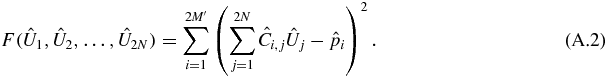
Cost function.
The cost function F is a function of 2N real variables (elements of the vector  ), which returns a real scalar. It is defined as follows:

or
Constraints.
The constraints, denoted as c, are nonlinear and are required to be input in the format

Equation (8) is rewritten as follows:

or

The ith row and the jth columns of Re([A]) and Im([A]) are defined as AR i,j and AI i,j, respectively. Similarly, let the jth row of Re({U}) and Im({U}) be defined as UR i,j and UI i,j, respectively.
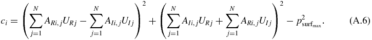
For all M nodes on the surface S, we require the acoustic pressure magnitude to be less than a specified threshold  . There are therefore M constraints associated with this condition. These can be expressed as follows.
For i ≤ M
In practice, numerical instability may arise if M is too large. In some cases, a subset of the nodes on S may have to be chosen.
In addition, the source velocity magnitudes cannot be greater than the maximum amplitude Umax allowed by the dynamic range. This is equivalent to adding the N further constraints.
For M < i ≤ M + N

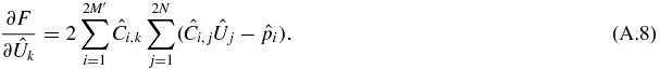
Gradient of cost function.
The gradient of the cost function with respect to its input variables may be expressed as follows.
For 1 ≤ k ≤ 2N,
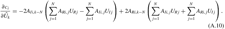
Gradient of constraints.
The gradient of the constraints with respect to the input variables forms a 2N by M + N Jacobian matrix (2N variables and M + N constraints). Its elements are as follows.
For k ≤ N and i ≤ M,
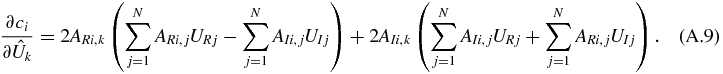
For k > N and i ≤ M,
For k ≤ N and i > M,


For k > N and i > M,

