
Abstract
This paper introduces a mouse atlas registration system (MARS), composed of a stationary top-view x-ray projector and a side-view optical camera, coupled to a mouse atlas registration algorithm. This system uses the x-ray and optical images to guide a fully automatic co-registration of a mouse atlas with each subject, in order to provide anatomical reference for small animal molecular imaging systems such as positron emission tomography (PET). To facilitate the registration, a statistical atlas that accounts for inter-subject anatomical variations was constructed based on 83 organ-labeled mouse micro-computed tomography (CT) images. The statistical shape model and conditional Gaussian model techniques were used to register the atlas with the x-ray image and optical photo. The accuracy of the atlas registration was evaluated by comparing the registered atlas with the organ-labeled micro-CT images of the test subjects. The results showed excellent registration accuracy of the whole-body region, and good accuracy for the brain, liver, heart, lungs and kidneys. In its implementation, the MARS was integrated with a preclinical PET scanner to deliver combined PET/MARS imaging, and to facilitate atlas-assisted analysis of the preclinical PET images.
Export citation and abstract BibTeX RIS
General scientific summary This paper introduces a mouse atlas registration system (MARS), composed of a stationary top-view x-ray projector and a side-view optical camera. This system uses the x-ray and optical images to guide an automatic co-registration of a mouse atlas with each subject, in order to provide anatomical reference for small animal molecular imaging systems. To facilitate the registration, a statistical atlas that accounts for inter-subject anatomical variations was constructed based on 83 organ-labeled mouse micro-CT images. The accuracy of the atlas registration was evaluated by comparing the registered atlas with the organ-labeled micro-CT images of the test subjects. The results showed excellent registration accuracy of the whole-body region, and good accuracy for the brain, liver, heart, lungs and kidneys. In its implementation, the MARS system was integrated with a preclinical PET scanner to deliver combined PET/MARS imaging, and to facilitate atlas-assisted analysis of the preclinical PET images.
1. Introduction
During the past several decades, in vivo molecular imaging of small animals has undergone rapid development in the preclinical research field. Conventional molecular imaging modalities such as positron emission tomography (PET) (Cherry 2001), single photon emission computed tomography (SPECT) (Ishizu et al 1995, Goorden and Beekman 2010), bioluminescence tomography (Wang et al 2006) and fluorescent molecular tomography (Ntziachristos 2006) have been increasingly used with small animals, especially mice. Novel molecular imaging modalities, such as optoacoustic tomography (Ntziachristos and Razansky 2010), Cerenkov luminescence tomography (Spinelli et al 2011) and magnetic particle imaging (Weizenecker et al 2009), are also emerging and are applied to the preclinical field.
The growth of small animal molecular imaging has also given rise to the need for anatomical imaging, which provides the anatomical information needed to help localize the molecular signal and assists quantification of tracer concentration. The role of in vivo preclinical anatomical imaging has primarily been accomplished through the use of micro-computed tomography (micro-CT) (Ritman 2011) and micro magnetic resonance imaging (micro-MR) (Driehuys et al 2008). Although micro-CT and micro-MR have contributed dramatically to preclinical imaging, their high cost and complexity prevent them from being readily combined with molecular imaging modalities. Great efforts have been made to combine micro-CT or micro-MR with molecular imaging systems (Catana et al 2006, Liang et al 2007, Guo et al 2010, Gulsen et al 2006), but such combinations increase the overall system cost, complexity and acquisition time. To address this problem, some researchers turned to the use of simpler anatomical imaging systems that lead to easier integration. Most of the simpler systems are composed of low-cost non-tomographic imaging devices, such as optical camera, 3D surface scanner and planar x-ray projector (McLaughlin and Vizard 2006). Although such systems cannot directly produce 3D anatomical images, they can guide the registration of a digital animal atlas as an anatomical reference to the molecular images. For example, the mouse atlas was registered with the body silhouettes captured by three optical cameras to guide organ-focused SPECT scans (Baiker et al 2009). There were also studies that use multiple-view optical photos (Zhang et al 2009) or video sequences (Savinaud et al 2010) to fuse mouse atlases with optical molecular imaging. To address the difficulty of capturing a complete body surface with optical cameras, a conical mirror design was used to acquire laser scans of the entire animal surface (Li et al 2009), and then guide the registration of the mouse atlas (Chaudhari et al 2007) to help with fluorescence tomography reconstruction.
In a previous study (Wang et al 2010), we simulated 11 different combinations of three non-tomographic imaging devices (i.e. optical camera, 3D surface scanner and planar x-ray projector) by positioning the devices at different view-angles to the subject. The accuracy of atlas registration was evaluated for each of the 11 combinations and the design of top-view x-ray plus side-view camera was among the most accurate choices. The top-view x-ray projection contains rich anatomical information on the body outline, the skeleton and the lungs. Some of the low x-ray contrast organs, such as the brain, heart, liver and kidneys, are all anatomically correlated with the body outline, skeleton and lungs. The side-view optical photo not only illustrates the body silhouette, it also reveals lateral spine curvature. Therefore, with a properly designed atlas registration method, the combination of top-view x-ray plus side-view camera could enable reasonable estimation of organ-level anatomy. It is also worth noting that a similar design of combining x-ray projection with optical cameras was proposed to capture the locomotion of rats (Duveau 2008) and to guide the registration of an articulated skeleton model (Gilles et al 2010). However, this study was not aimed at combining molecular/anatomical imaging and it required implanted x-ray markers to capture the animal motion.
Based on the previous simulation study, we introduce here the mouse atlas registration system (MARS) with a top-view x-ray projector and a side-view optical camera. To encompass differences in animal shapes and sizes, instead of using a single subject atlas, we developed a statistical atlas based on 83 segmented mouse CT images. The statistical shape model (SSM) and conditional Gaussian model (CGM) techniques were used to automatically register this new atlas without any user intervention with the x-ray projection and the camera photo. The MARS was also combined with the PETbox4 scanner (Gu et al 2011) to provide integrated PET/MARS imaging.
2. Materials and methods
2.1. System setup
As shown in figure 1(a), the MARS is composed of a top-view planar x-ray projector and a side-view optical camera. Unlike tomographic CT systems, the MARS is stationary. Only one single x-ray projection and one optical photo need to be taken for the subject; therefore the acquisition time is only a few seconds. Figure 1(b) demonstrates the hardware components of the MARS. The whole system is enclosed in a steel box of 305 × 254 × 125 mm3 for x-ray shielding. A miniature x-ray tube (MAGNUM® 40 kV x-ray source, Moxtek Inc., UT, USA) is placed 238 mm above the center of the mouse field of view (FOV), and the x-ray detector (RedEye™ 200 Remote Sensor, Rad-icon Imaging Corp. CA, USA) with 98 × 96 mm2 imaging area is placed 45 mm under the FOV center. The distances of the x-ray source and detector are designed to capture the main body (from nose to the root of the tail) of a medium sized (∼25 g) laboratory mouse. To eliminate the very low-energy x-rays which mostly contribute to soft tissue dose, a 1 mm thick aluminum filter is placed on top of the collimator. The x-ray tube configuration is set at 40 kVp, 100 µA and 3 s exposures. The voltage and current used here are much lower than those used for a commercial micro-CT system, and the single-view x-ray projection delivers significantly less radiation than a fully tomographic CT (e.g. about 1/450 of the dose delivered by a CT scan of 70 kVp, 500 µA for 10 min).

Figure 1. Design of the MARS. (a) Concept drawing of the MARS. (b) Hardware components of the MARS with the front cover of the box removed. (c) The MARS box in working status, with the front cover on, coupled to the PETbox4 scanner. The mouse chamber moves through the FOV of the two systems for combined imaging.
Download figure:
Standard imageFor the optical part, a webcam (Firefly® MV, Point Grey Research Inc., BC, Canada) with a 5 mm focal length lens is placed 185 mm laterally to the right side of the FOV center. The camera exposure time is set to 200 ms and LED backlights with a thin piece of light diffuser are positioned on the left side of the mouse. The backlight highlights the body silhouette during the photo acquisition.
Figure 1(c) shows the MARS box in operation. A multi-modality animal imaging chamber similar to that used in previous work (Suckow et al 2009) with anesthesia and heating support is used for the image acquisition. The chamber also maintains the subjects in a regularized posture, i.e. with stretched limbs and prone position. For imaging, the mouse chamber first enters the MARS box, the x-ray projection is acquired for 3 s, followed by a snapshot from the optical camera. Figure 1(c) also shows that the MARS box is combined with the PETbox4 system (Gu et al 2011), a bench-top preclinical PET scanner developed by our group. For combined imaging, the MARS box is simply positioned in front of the PETbox4, with collinear openings that allow the imaging chamber with the mouse subject to move freely between the two systems. Combined PETbox4/MARS images are shown in the results.
2.2. Geometric calibration of the MARS
Both the x-ray projector and optical camera were calibrated as pinhole systems. The geometric parameters of the pinhole systems were calibrated with a planar checkerboard (figure 2(a)) visible to both the x-ray and the optical camera. The checkerboard was designed as a 7 × 7 square pattern and the dimension of each square was 6 × 6 mm2. The PCB production technique was used to etch the checkerboard pattern of copper onto the substrate. The geometric parameters to be calibrated included intrinsic and extrinsic parameters. The intrinsic parameters included the focal length, principal point, image skew and distortions of each pinhole system. The extrinsic parameters included the translation and rotation of each pinhole system with respect to the world coordinate system. To calibrate the intrinsic parameters, multiple (10–20) random positions and orientations of the checkerboard were captured separately by each system. Figure 2(b) demonstrates a result of the intrinsic parameter calibration, where the barrel distortion of the side-view photo is eliminated after taking into account the intrinsic distortion (for the top-view x-ray there is no appreciable image distortion). To calibrate the extrinsic parameters, the checkerboard was positioned at an oblique angle so that both systems could image it simultaneously. The common coordinate space of the two systems was determined based on this oblique checkerboard position (figure 2(c)), with the origin defined at the upper-left corner of the checkerboard (facing the operator), the x- and y-axes defined parallel with the checkerboard edges, and the z-axis defined perpendicular to the checkerboard plane. The Camera Calibration Toolbox for Matlab® was used to calculate the intrinsic and extrinsic parameters based on the multiple x-ray and optical checkerboard images. The toolbox requires the checkerboard size and the square number as inputs, while no information on checkerboard positions was required. The user needs to manually specify the four corners of the checkerboard in each image, then the method will automatically search for the corners of each individual square and compute the optimal intrinsic and extrinsic parameters that match the square corners. For details of the calibration method used by the toolbox, we refer the readers to Zhang (1999) and Heikkila and Silven (1997). To define the common coordinate space (i.e. the world coordinate space), the angle and position of the checkerboard do not need to be unique, because the world coordinate system is only a connection between the atlas coordinates and the projection coordinates. Moreover, since the MARS is designed to be combined with molecular imaging systems, it is necessary to co-register the MARS world coordinate system with the molecular imaging system. For the specific application of this paper, we co-register the MARS with the PETbox4 scanner using four 22Na point sources that were fixed in the imaging chamber. The point sources were imaged with both MARS and PETbox4, and the source positions in both MARS and CT images were manually specified. The 3D coordinates of the point sources in MARS space were calculated by back-projecting the 2D coordinates into 3D, and then the 3D rigid transformation (including translation and rotation) between the two point sets (MARS and CT) was calculated.
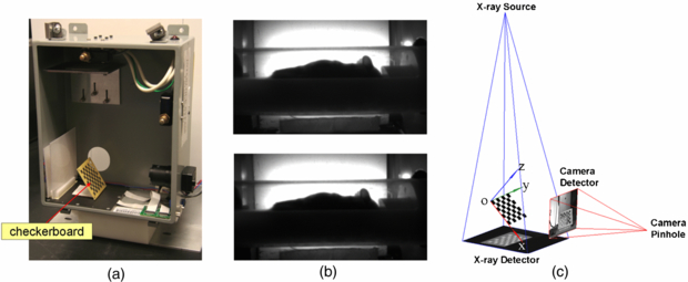
Figure 2. Geometrical calibration of the MARS. (a) The checkerboard used for calibrating both the x-ray projector and the optical camera. (b) An example of the intrinsic parameter calibration result, the barrel distortion in the raw photo (upper row) is eliminated (lower row) after taking into account the intrinsic distortion factor. (c) The calibrated pinhole models of the x-ray projector and the optical camera. The common coordinate space of the two devices is based on an oblique checkerboard position. In this figure the camera pinhole model is magnified 16 times to clearly show the checkerboard photo.
Download figure:
Standard image2.3. Preprocessing of mouse x-ray and optical images
The x-ray image (figure 3(a)) and the optical photo (figure 3(d)) are preprocessed before atlas registration. The perspective and barrel distortions of the acquired images are corrected using the geometric calibration parameters. Moreover, since the mouse is imaged along with the chamber, we need to eliminate the chamber from both the x-ray and optical images. An additional x-ray projection of the empty chamber (figure 3(b)) is acquired and eliminated from the subject x-ray image. Let Imc be the x-ray image of the mouse and chamber, Ic be the x-ray image of the empty chamber and Id be the dark current image of the x-ray detector. The chamber-eliminated image of the mouse Im (figure 3(c)) can be calculated as Im = (Imc − Id)/(Ic − Id). In the side-view backlit optical photo, lower parts of the mouse body are blocked by the chamber, leaving only the back region and upper head visible to the camera. Therefore, a rectangular region (figure 3(d)) enclosing the visible body part is used for atlas registration. An automatic thresholding method (Bersen 1986) is applied to the selected region to extract the body silhouette (figure 3(e)). The acquisition of the empty chamber x-ray and the manual determination of the optical rectangular region must be performed only once for each MARS gantry, since the position of the chamber is always fixed to the gantry, similar to previous work by our group (Chow et al 2006).
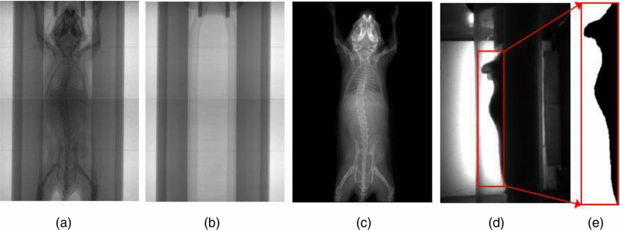
Figure 3. Preprocessing of the MARS images. (a) The x-ray image of a mouse in the chamber. (b) The x-ray image of the empty chamber. (c) The x-ray image after eliminating the chamber. (d) The side-view optical photo of the mouse in the chamber. The rectangular region encloses the body part visible to the camera. (e) Segmentation of body silhouette from the rectangular region of (d).
Download figure:
Standard image2.4. Registration of a statistical mouse atlas
The limited mouse area visible in the side-view photo reduces the completeness of the acquired data, making direct application of the atlas registration method described in our previous simulation study (Wang et al 2010) unfeasible. To solve this problem, we constructed a statistical mouse atlas based on multiple training subjects, and fit the atlas to the incomplete data using the techniques of SSM and CGM. Since this method is similar to the approach that we used for CT-based atlas registration, here we only briefly introduce this method and refer the readers to Wang et al (2012) for more details.
The statistical mouse atlas was trained with 83 organ-labeled micro-CT images selected from the database at the Crump Institute for molecular imaging, UCLA (Stout et al 2005). The training subjects include three most frequently used strains (Nude, BC57 and severe-combined immunodeficient (SCID)), with body weights ranging from 15 to 30 g. The liver contrast agent Fenestra™ (ART, Quebec, Canada) was injected intra-venously into the training subjects to provide better CT contrast of abdominal soft tissues. Major organs, including the skin, skeleton, lungs, heart, brain, liver, spleen and kidneys, were segmented from these training CT images. Triangular meshes of the segmented organs were generated and the SSM was constructed as the point distribution model of the mesh vertices:

where S is a shape instance of the model and  is the mean shape. The shape is represented as a vector that lines up the coordinates of all the mesh vertices. V is the matrix of the shape variation modes, which are obtained using the principal component analysis of the mesh vertices, and b represents the shape coefficients that control the linear combination of the variation modes. By optimizing the value of b, the shape model can be fited to the individual subject images, which in our case are the x-ray image and side-view silhouette.
To register the atlas with the MARS images, a hierarchical approach is used (as shown in figure 4), i.e. the organs with high x-ray contrasts are registered first, and then the low x-ray contrast organs are mapped according to the registered high contrast organs.
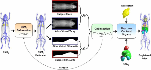
Figure 4. Workflow of the 2D/3D registration of the statistical mouse atlas with the MARS images. The SSM (SSM1) of the high contrast organs (i.e. the skin, skeleton and lungs) is first registered with the x-ray and optical silhouette, and then the low contrast organs (including the brain, heart, liver, spleen and kidneys) are mapped according to the registered high contrast organs.
Download figure:
Standard imageTo register the high contrast organs, a SSM, namely SSM1, is constructed for the skin, skeleton and lungs. For initialization, the mean shape of SSM1 is roughly positioned at the subject location of the MARS gantry. This initialization needs to be performed only once for a fixed gantry. The deformation of SSM1 is described by the vector T = [l, b], where l is a nine-element 3D linear transformation, including three translations, three rotations and three anisotropic scaling factors; b is the shape coefficient of SSM1, which contains 24 principal components that represent 95% of the training set variations. The initial values of l and b are set to identity transform and 0, respectively. The registration is executed iteratively. For each iteration, the virtual x-ray projection and side-view silhouette of the atlas are generated using the fast mesh projection method (Wang et al 2010), based on the geometric calibration parameters of the x-ray projector and the optical camera, respectively. The similarity (fX) between the atlas x-ray projection and the individual x-ray projection is measured with mutual information (Wells et al 1996), and the similarity (fS) between the atlas silhouette and the individual silhouette captured by the optical camera is measured with 1-Kappa, where Kappa is the Kappa statistics (Klein and Staring 2011) that measures the overlapping ratio between two binary regions. The combined similarity between the deformed atlas and the individual subject is calculated as f = fX + fS. Here we use equal weights for fX and fS because they are considered equally important for the registration. Although the x-ray provides more anatomical information than the optical silhouette, the side-view silhouette also implies the lateral curvature of the spine, which is important for defining the 3D spine curvature. The Powell method (Powell 1964) is used to obtain the optimal value of T (i.e. T* in figure 4) that minimizes the value of f. A multi-resolution scheme is used to accelerate the registration and to avoid convergence to local minima. Three resolution levels are used, and the down-sampling ratios of the three levels are 4, 2 and 1.
After the high contrast organs are registered, the brain mesh borrowed from the Digimouse atlas (Dogdas et al 2007) is mapped with the 3D thin-plate-spline interpolation, using the skull vertices as the control points. To map the heart, liver, spleen and kidneys, a SSM, namely SSM2, is constructed for those organs. The anatomical correlation between SSM1 and SSM2 is learned from the training set using the CGM. Given the shape coefficients of SSM1 fitted to the individual subject, the CGM is used to predict the shape coefficients of SSM2, so that SSM2 is also fitted to the individual subject.
2.5. Evaluation of the atlas registration accuracy
The accuracy of the mouse atlas registration was evaluated by comparing the registered atlas with the segmented micro-CT images of five test subjects. The test subjects included three commonly used strains (Nude, SCID and BC57s) and covered the weight range of 18–33 g. The subjects were injected with minimal dose of Fenestra™ LC (Suckow and Stout 2008) to maintain reasonable CT contrast without undermining the spine contrast in the MARS x-ray projection images. For each subject, the MARS scan was acquired first, and then the imaging chamber with the mouse subject was transferred to a micro-CT system (microCAT II, Siemens Preclinical Solutions, Knoxville, TN, USA) for a tomographic CT scan. During both MARS and CT scans, the subjects were kept anesthetized in the chamber to minimize posture changes. Based on the reconstructed CT images, major organs were manually segmented by a human expert. To establish the transformation from the CT coordinate space to the MARS coordinate space, the skin mesh of the segmented CT was mapped into the MARS space by a linear matrix M, which represents the translation and rotation in 3D space. The values of translation and rotation were manually fine-tuned until the top-view and side-view projections of the skin mesh matched well with the body outlines in the MARS images. Finally the inverse of M was used to map the registered atlas into the CT space, and the overlapping ratios between the atlas organs and the segmented CT organs were measured using the Dice coefficient,

where RA and RS represent the organ region of the registered atlas and the expert segmentation, respectively (| · | denotes the number of voxels and ∩ means the overlapping between two regions). The Dice coefficient has the value range of [0, 1], where 1 corresponds to complete overlapping and 0 corresponds to no overlapping.
To measure the accuracy of registered organ volume, the recovery coefficient of organ volume (RCvlm) was used,

where VA and VS are the organ volumes of the registered atlas and the expert segmentation, respectively.
The surface distances between the registered atlas organs and the expert segmented organs were measured by the averaged surface distance (ASD),

where nA and nS are the numbers of vertices in the surface meshes of the registered atlas and the expert segmentation, respectively. di is the minimum distance from the ith vertex of the atlas surface to all the vertices of the expert segmentation surface and dj is the minimum distance from the jth vertex of the expert segmentation surface to all the vertices of the atlas surface. Based on this definition, smaller ASD means better registration accuracy.
3. Results
3.1. Atlas registration accuracy
Table 1 reports the Dice coefficients of the major organs of the five test subjects. The strain and weight information of the animal is also listed. As reflected from the Dice results, the first subject had the best overall accuracy, while the second subject had the worst overall accuracy. Larger organs such as the whole body, the brain and the liver generally have better registration accuracy, while smaller or long-shape organs such as the spleen or skeleton normally have poorer registration accuracy. For visual illustration, the registration results of the best (subject 1), average (subject 4) and worst accuracies (subject 2) are shown in figure 5. Organ outlines of the registered atlas are projected onto the x-ray and optical images. The low contrast organs are not projected since it is impossible to visually compare these organs with the atlas projections in the MARS images.

Figure 5. Examples with the best (left), average (middle) and worst (right) registration accuracies of the test subjects. Organ outlines of the registered atlas are projected onto the x-ray and optical images.
Download figure:
Standard imageTable 1. Animal information and organ Dice coefficients for the five test subjects.
| Dice | |||||||||||
|---|---|---|---|---|---|---|---|---|---|---|---|
| Subject | Strain | Weight (g) | Whole body | Skeleton | Lungs | Brain | Heart | Liver | Spleen | Left kidney | Right kidney |
| 1 | Nude | 26.8 | 0.89 | 0.35 | 0.63 | 0.75 | 0.89 | 0.54 | 0.30 | 0.57 | 0.64 |
| 2 | SCID | 33.1 | 0.80 | 0.18 | 0.59 | 0.48 | 0.53 | 0.49 | 0.13 | 0.51 | 0.47 |
| 3 | BC57 | 18.4 | 0.84 | 0.39 | 0.57 | 0.62 | 0.49 | 0.64 | 0.28 | 0.62 | 0.72 |
| 4 | BC57 | 19.2 | 0.83 | 0.39 | 0.71 | 0.78 | 0.46 | 0.60 | 0.34 | 0.52 | 0.73 |
| 5 | BC57 | 20.1 | 0.81 | 0.35 | 0.59 | 0.73 | 0.47 | 0.53 | 0.11 | 0.44 | 0.71 |
| Mean | 23.5 | 0.83 | 0.33 | 0.62 | 0.67 | 0.57 | 0.56 | 0.23 | 0.53 | 0.65 | |
| Std | 6.31 | 0.04 | 0.09 | 0.06 | 0.12 | 0.18 | 0.06 | 0.10 | 0.07 | 0.11 | |
Table 2 reports the RCvlm of the major organs of the five test subjects. Unlike the Dice coefficients, the RCvlm does not present an obvious subject-dependent distribution. The mean RCvlm of all the organs falls into the range of [0.9, 1.3], which means reasonably good estimations of the organ volumes. In terms of standard deviation, the whole body and the brain demonstrate smallest deviations (0.04 and 0.06, respectively) across the test subjects, while the spleen has the largest deviation (0.35).
Table 2. Organ volume recovery coefficients (RCvlm) for the five test subjects.
| RCvlm | |||||||||
|---|---|---|---|---|---|---|---|---|---|
| Subject | Whole body | Skeleton | Lungs | Brain | Heart | Liver | Spleen | Left kidney | Right kidney |
| 1 | 1.01 | 1.18 | 1.05 | 1.09 | 1.05 | 0.93 | 1.02 | 1.04 | 0.97 |
| 2 | 1.07 | 0.91 | 1.08 | 1.09 | 1.25 | 1.03 | 1.48 | 1.19 | 1.10 |
| 3 | 1.04 | 0.92 | 1.30 | 1.04 | 0.94 | 1.12 | 0.89 | 1.43 | 1.19 |
| 4 | 1.10 | 0.80 | 1.03 | 1.08 | 1.24 | 1.16 | 1.26 | 1.28 | 1.28 |
| 5 | 1.02 | 0.82 | 1.40 | 0.95 | 0.95 | 1.35 | 0.58 | 1.13 | 1.03 |
| Mean | 1.05 | 0.93 | 1.17 | 1.05 | 1.09 | 1.12 | 1.05 | 1.21 | 1.11 |
| Std | 0.04 | 0.15 | 0.17 | 0.06 | 0.15 | 0.16 | 0.35 | 0.15 | 0.12 |
Table 3 reports the ASDs of the major organs of the five test subjects. For all the organs, the mean ASD falls into the range of [0.83, 1.35], meaning the registration accuracy is around 1 mm. Similar to the Dice coefficient results, subject 2 showed worst (largest) ASDs for most organs. It can also be seen that the spleen and the skeleton do not have much worse (larger) mean ASDs than the other organs, which are different from the Dice results. Such a finding suggests that the spleen and the skeleton have got reasonably close registration, but their curved shapes led to imperfect volumetric overlapping ratios.
Table 3. Organ ASD for the five test subjects (unit: mm).
| ASD (mm) | |||||||||
|---|---|---|---|---|---|---|---|---|---|
| Subject | Whole body | Skeleton | Lungs | Brain | Heart | Liver | Spleen | Left kidney | Right kidney |
| 1 | 1.26 | 0.98 | 0.67 | 1.04 | 1.28 | 0.66 | 1.00 | 0.74 | 0.84 |
| 2 | 1.17 | 0.95 | 1.16 | 0.85 | 1.64 | 2.02 | 1.56 | 1.62 | 1.50 |
| 3 | 0.98 | 0.71 | 0.71 | 0.87 | 1.08 | 0.76 | 0.82 | 0.73 | 0.76 |
| 4 | 1.03 | 0.79 | 0.67 | 0.66 | 1.33 | 0.72 | 1.00 | 1.10 | 0.90 |
| 5 | 1.18 | 0.84 | 0.69 | 0.53 | 1.16 | 0.89 | 0.85 | 1.47 | 1.15 |
| Mean | 1.13 | 0.87 | 0.83 | 0.86 | 1.35 | 1.10 | 1.09 | 1.12 | 1.01 |
| Std | 0.12 | 0.11 | 0.22 | 0.13 | 0.20 | 0.28 | 0.58 | 0.39 | 0.29 |
The atlas registration accuracy of this study was also compared with two previous studies, i.e. our previous simulation study that compares different combinations of the non-tomographic imaging devices (Wang et al 2010) and the study that registered the statistical mouse atlas with fully in tomographic CT images (Wang et al 2012). The purpose selecting these two studies was to determine whether the performance of the MARS agrees well with the simulation design, and also to compare the MARS-based atlas registration with a fully tomographic CT-based atlas registration. Figure 6 illustrates the comparison of the means and standard deviations of the organ Dice coefficients. It can be seen that the MARS performance of this study is within the statistical margin of error of the simulation design. For some of the organs, such as the lungs, the spleen and the kidneys, this study has slightly better mean Dice coefficients than the simulation study, while for the rest of the organs the simulation study is better. For the 'CT registration' study the Dice coefficients of the whole body, skeleton and brain were not available, since that study only focused on the trunk region. However, for the available organs, it is obvious that the mean values of the CT-based registration are larger than those of the MARS-based registration. This finding illustrates the tradeoff between accuracy of atlas registration and system complexity, cost and radiation dose by using a simpler imaging system than fully tomographic CT.
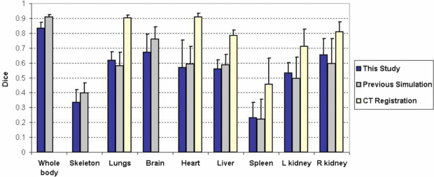
Figure 6. Comparison of the atlas registration accuracy of this study with two previous studies. For each study, the mean and standard deviation of the organ Dice coefficients are plotted. The 'previous simulation' refers to our simulation study for assessing the registration accuracy based on top-view x-ray projection and side-view optical photo (Wang et al 2010). The 'CT registration' refers to the approach of registering the statistical mouse atlas to full tomographic CT images (Wang et al 2012). The 'CT registration' study only focused on the trunk region; therefore no Dice coefficients of whole body, skeleton and brain were available.
Download figure:
Standard imageThe registration algorithm was programmed with C++, and took 3–4 min for each subject on a desktop PC with 3.05 GHz CPU and 6 GB RAM, using a single CPU thread.
3.2. Combined imaging with PETbox4
As introduced in section 2.1, the MARS can be easily combined with a molecular imaging system, such as the PETbox4 tomograph. Figure 7 shows an example of a registered atlas overlaid with the PETbox4 image. A 30 g mouse was injected with ∼50 µCi [18F]FDG 1 h before the scan. The registered atlas was converted to a volumetric image by filling the organ meshes with pseudo CT Hounsfield values (as shown in figures 7(a) and (b)). The volume rendering of the registered atlas overlaid with the PET signal is shown in figure 7(c). With the combined PET/MARS images, the atlas not only provides anatomical reference for the PET image, it also offers initial organ regions for quantifying the PET organ uptakes, but an evaluation of this is out of the scope of this paper.

Figure 7. Visualization of registered atlas (gray scale) overlaid with PETbox4 images from a mouse injected with [18F]FDG (rainbow colors). (a) Coronal view. (b) Sagittal view. (c) Volume rendering.
Download figure:
Standard image4. Discussion
As shown from tables 1–3 and figure 5, the MARS-based atlas registration achieves promising accuracy. For the subjects with the best and average accuracy, the registered atlases demonstrate good alignment of the skin, skeleton and lungs with the x-ray images and optical photos. It can also be observed that in the side-view photo, in spite of the partially obscured body silhouette caused by the imaging chamber, the registration method can recover the missing silhouette region by fitting the SSM. This finding confirms the advantage of using the shape model for a non-tomographic system, i.e. the inadequacy of acquired data can be partially compensated by anatomical priors.
Among all the test subjects, the second subject presents the worst accuracy (in terms of both Dice and ASD) for most of the organs. The main reason is that the weight of this subject (33.1 g) is beyond the weight range of the atlas training set (15–30 g). Although anisotropic scaling (the linear transformation l of section 2.5) has been used to compensate for the size (or weight) difference between the atlas and the subject, this scaling cannot fully compensate for the nonlinear shape changes caused by animal growth. The best solution to this problem will be to incorporate more large weight subjects into the atlas training set, which is planned for future studies. Moreover, based on the current results, it seems that subject weight is a major factor that affects the registration accuracy, but the influence of animal strain and sex is unclear. In a future study, group-wise atlases for different weights, ages, strains and sexes will be constructed and evaluated for registration accuracy.
Figure 6 demonstrates the averaged Dice coefficients across the test subjects of this study. Among all the organs, the whole-body region achieves the largest Dice coefficient (≥0.80 for all the test subjects) and good RCvlm (1.05 ± 0.04). Such high whole body accuracy will be helpful to some molecular imaging modalities that need good estimation of the body, for example for the attenuation correction of mouse preclinical PET or SPECT (especially when the radiolabeled probe does not have enough concentration to show the body outline), and the reconstruction of optical tomography data (Song et al 2007). In contrast to the high Dice coefficients of the whole-body region, the skeleton generally has poor Dice coefficients (<0.4), although its RCvlm (0.93 ± 0.15) and ASD (0.87 ± 0.11 mm) are reasonably accurate. The reason is that the skeleton is composed of several long-curve-shaped parts such as the spine and the limbs, which are very difficult to align accurately. Slight deviations of the spine curvature or the limb directions lead to significant decreases of the Dice coefficient. The skull does not have a long-curved shape; therefore it is better aligned. The accuracy of the skull can be indirectly reflected from the accuracy of the brain (Dice coefficient = 0.67 ± 0.12, RCvlm = 1.05 ± 0.06, ASD = 0.86 ± 0.13 mm), since the brain and the skull are anatomically closely correlated.
As for the soft organs, the lungs have moderate Dice coefficients (0.62 ± 0.06) and RCvlm (1.17 ± 0.17), due to their complex shape and flexible size. The heart and the liver are anatomically correlated with the lungs; therefore they have similar level of Dice coefficients as the lungs. The spleen has the worst Dice coefficient (0.23 ± 0.10), as well as the most variable RCvlm (1.05 ± 0.35) and ASD (1.09 ± 0.58 mm) among all the organs, because its long and curved shape makes it difficult to get a good volumetric overlapping. It is noticeable that the left and right kidneys have different levels of Dice coefficients and ASDs for all the test subjects. This is because the position of the right kidney is highly correlated with the liver, while the left kidney is correlated with the spleen. The liver is a big organ with stable position, while the spleen is more movable. As a result, the right kidney has better accuracy than its left counterpart in terms of both mean Dice and ASD.
Based on figure 6, the results of this study are compared with the previous simulation study. The Dice coefficients calculated are approximately at the same level of the simulation results. Since different registration methods were used for the two studies, the organ accuracies cannot be exactly the same. The previous simulation study used free-form deformations (FFD) for atlas registration, while this study uses a shape-model-fitting method due to the incompleteness of side-view silhouette. The FFD is good at matching curved-shape structures such as the spine and the limbs, while the shape model is inferior at matching these structures since the anatomy of the model is constrained within the training set. This is also the reason that the shape-model-based method requires a dedicated chamber to regularize the subject posture. Nevertheless, for the estimation of low contrast organs, the shape-model-based method has the advantage of producing plausible organ shape, while the FFD-based method tends to slightly distort the organ shapes, especially for the kidneys whose shapes can be deformed by skin matching. Therefore the shape-model-based method has better accuracies for the kidneys. In future research, it would be promising to combine the FFD with the shape model, so as to further improve the registration accuracy.
Figure 6 also reveals that the CT-based atlas registration is more accurate than the MARS-based registration. Compared with the CT, the MARS has simpler system design, lower cost, reduced acquisition time and less radiation dose. However, the CT provides full tomographic anatomical information, leading to more accurate atlas registration. There is a trade-off between the system simplicity and the atlas registration accuracy. For future studies, it might be worthwhile to investigate methods to moderately increase the MARS complexity to gain better registration accuracy. For example, adding one more x-ray projection to acquire more anatomical information, and/or adding a surface scanner to acquire surface geometry. As discussed before, the side-view photo is partially obscured by the chamber; therefore replacing the side-view camera with an x-ray projector will also provide more complete anatomical information, although such replacement will slightly increase the gantry width (from 254 to 305 mm) and double the system cost.
Another concern on the use of the MARS may arise from the registration of diseased subjects with an atlas of healthy subjects. Many preclinical studies are conducted with diseased mouse models, in which the organ anatomy may be altered. For example, a tumor on the body surface may change the overall body shape, and a sick mouse may have larger spleen than normal (as an immune response to the disease). For these cases, on one hand the atlas can provide a healthy reference to be compared with the diseased phenotype, but on the other hand the healthy atlas is inadequate for matching the diseased anatomy. To address these problems, adding a surface scanner may help in capturing the surface tumor shape, and building a special atlas for common diseased mouse models (such as with big spleen) may also be a candidate solution.
The development of the MARS offers a new perspective on small animal anatomical imaging. As shown by the combined PETbox4/MARS imaging, the integration of the MARS with a molecular imaging system is simple and straightforward. The MARS provides fully unsupervised registration of an anatomical atlas with the molecular imaging modality. Since no user intervention is needed for the registration, the procedure of molecular image analysis is greatly simplified. Compared with conventional human-expert-based organ labeling, the MARS-based approach is less labor-intensive, more objective and should be more reproducible. Moreover, the MARS-based approach also allows the localization of the dark organs which are not well visible in the molecular images (such as the liver in [18F]FDG PET image), while a human expert may have difficulty contouring those dark organs. For the purpose of PET organ uptake quantification, one would desire the organ ROI be as accurate as possible. As demonstrated by the test results, the MARS does not provide enough accuracy for direct quantification of most organs, but even the CT-based registration accuracies are not sufficient for some low-Dice organs (e.g. the spleen). Nevertheless, the important contribution of MARS is that it provides size-appropriate close ROI initialization, which is the prerequisite of atlas-based organ segmentation and quantification in PET images (Rubins et al 2003, Kesner et al 2006). Moreover, the organ ROIs provided by MARS can also be used for other applications that require lower registration accuracy, such as locally focused scanning (Baiker et al 2009) and combined functional/anatomical visualization (Khmelinskii et al 2010). Overall, we hope this work could enrich the design of modern preclinical molecular imaging systems and improve the quality of molecular imaging data analysis.
5. Conclusion
This paper introduces an atlas-based mouse anatomy imaging system with a top-view x-ray projector and a side-view optical camera. The system design is simple, and can be easily combined with molecular imaging modalities, such as preclinical PET. With the specially designed statistical mouse atlas registration method, the system provides a registered mouse atlas as an estimation of the individual anatomy. Experimental studies based on real mice illustrate the effectiveness of this system. Future directions will focus on increasing the atlas registration accuracy with a more comprehensive atlas, more advanced registration methods and improved system design.
Acknowledgments
The authors would like to thank Waldemar Ladno and Darin Williams for help with animal experiments and Dr Robert Silverman, Dirk Williams and Wesley Williams for designing and manufacturing the MARS box. We appreciate the helpful discussions from Dr Ritva Lofstedt, Alex Dooraghi and Brittany Berry-Pusey. A provisional patent application describing parts of the 2D/3D atlas registration has been filed (UCLA Case no 2011-395). The design of the MARS has been commercialized by Sofie Biosciences Inc., Culver City, CA, USA. This work was supported in part by SAIRP NIH-NCI 2U24 CA092865 and in part by a UCLA Chancellor's Bioscience Core grant.