


Abstract
Experiments on HL-2A, DIII-D and EAST show that turbulence just inside the last closed flux surface acts to reinforce existing sheared E × B flows in this region. This flow drive gets stronger as heating power is increased in L-mode, and leads to the development of a strong oscillating shear flow which can transition into the H-mode regime when the rate of energy transfer from the turbulence to the shear flow exceeds a threshold. These effects become compressed in time during an L–H transition, but the key role of turbulent flow drive during the transition is still observed. The results compare favourably with a reduced predator–prey type model.
Export citation and abstract BibTeX RIS
1. Introduction
Operation in the high confinement mode (H-mode) is a key part of the baseline operating scenario for ITER. The development of a reliable physics-based macroscopic power threshold model for access to H-mode requires an understanding of the underlying mechanism that leads to the formation of the H-mode regime. Recent work has shown that an intermediate limit cycle oscillation (LCO) regime (which is sometimes termed an intermediate or I-phase) can develop [1] during the transition to H-mode. The LCO is characterized by short period (<1 ms) oscillations in both the turbulence amplitude and the sheared low-frequency (LF) poloidally/toroidally symmetric (m, n = 0) Er(t) × B0 flow denoted by
 in the region ∼1–2 cm inside the last closed flux surface (LCFS), and by variations in cross-field transport and divertor Da light emissions. These dynamics co-exist with and include the slowly evolving (many msec to many tens of msec) m, n = 0 E × B shear flow associated with the ion pressure gradient via the radial force balance, sometimes denoted as either the diamagnetic E × B flow, Vdia, or mean shear flow, VMSF. These observations have been interpreted as being qualitatively consistent with a predator–prey model of the L–H transition [2]. However, to date no direct measurement of the development and evolution of the key physics quantity in this model—the Reynolds stress mediated transfer of turbulent kinetic energy to
 , also known as the power transfer or shear flow production
 —have been made in strongly heated L-modes, in the LCO or during the H-mode transition. This paper provides such results from work in the HL-2A, DIII-D and EAST tokamak devices. The results provide significant support for the predator–prey model, suggesting a pathway to a physics-based understanding of the L–H transition.
2. Theoretical background
The evolution of the turbulent and m, n = 0 sheared E × B flow kinetic energies, denoted
 and
and
 respectively, can be viewed as a simple power balance between the turbulent scale and the zonal flow scale. Due to pressure gradient-driven instabilities, fluctuation power is input into the finite (m, n) turbulence scales from the pressure gradient which acts as a free energy source. Some of this power is transferred to small spatial scales (i.e. high frequency/high wavenumber) and some into the m, n = 0 sheared flows where it is then dissipated by viscous or flow-damping mechanisms, respectively. The power balance for the turbulent scale and m, n = 0 shear flow scales can then be written in terms of two equations:
where the effective turbulence energy input rate is given by γeff = γeff (∇n, ∇T, V'E, ...), the m, n = 0 E × B flow-damping rate is given by γZF, and the plasma-frame decorrelation rate by
 , indicating the rate of nonlinear energy transfer to the high k region where viscous dissipation occurs. The power transfer or production term PLF has already been introduced above, and appears as a sink in the first equation and a source in the second equation. We note that this simple power balance model for the turbulence/sheared E × B system reduces to the published predator–prey model [2] if the input rate is given as
 where γl = γl (∇n, ∇Ti,e) is the linear growth rate of the gradient-driven instability in the absence of flow shear, the pressure gradient is given as ∇pi ∝ qi where the control parameter qi denotes the heat flux through the system, the mean shear flow is proportional to the curvature of the pressure profile, i.e.
 , the stress is taken to scale as PLF and α is a constant parameter. Estimates for γeff can be obtained from measurements of
 and
and
 , or it can be modelled. The production term PLF is determined via an approach similar to that used in earlier work [3] in which the relevant quantities are computed in the time-domain using suitably filtered and averaged quantities. This approach implicitly assumes that there is a separation of timescales (or equivalently frequency) between the turbulent and m, n = 0 sheared E × B flow scales, which in turn requires a priori knowledge of the relevant timescales. For the HL-2A, EAST and DIII-D devices these scales have previously been identified (see e.g. [4–6]). We also point out that this zero-dimensional model neglects the divergence of triple product terms in the energy balance model equations [7] which correspond to turbulence amplitude spreading and turbulent scattering of shear flow.
2.1. Model behaviours
When
 this system has a fixed-point solution given approximately as
![$V_{E\times B}^{\rm LF} = [\langle \tilde{v}_{\perp}^2 \rangle(\gamma_{\rm eff} -\gamma_{\rm decorr}^{\rm pl})/\gamma_{\rm LF}]^{1/2}$](https://content.cld.iop.org/journals/0029-5515/53/7/073053/revision1/nf460410ieqn012.gif) . A slow increase in the heat flux (e.g. slow enough so that the edge gradients evolution is slow compared with the confinement time) should then increase the density and temperature gradients and heat the edge, resulting in an increase in the turbulence amplitude and a decreased rate of zonal flow damping γZF. As a result
. A slow increase in the heat flux (e.g. slow enough so that the edge gradients evolution is slow compared with the confinement time) should then increase the density and temperature gradients and heat the edge, resulting in an increase in the turbulence amplitude and a decreased rate of zonal flow damping γZF. As a result
 ,
,
 and PLF should grow with increased heating power under fixed-point L-mode conditions. We note that recent studies in L-mode discharges have confirmed this behaviour [8]. When
 , a growing solution
 can now exist and thus
can begin to grow at the expense of the turbulent energy
, signalling the onset of the LCO regime. If the energy transfer rate becomes strong enough so that
can now exist and thus
can begin to grow at the expense of the turbulent energy
, signalling the onset of the LCO regime. If the energy transfer rate becomes strong enough so that
 , then the turbulence amplitude (and thus the turbulent-driven cross-field transport) can collapse, resulting in a quenching of turbulent transport and an increase in the ion pressure gradient and the MSF. As noted above, in the predator–prey model the effective energy input rate is decreased by the mean shear flow, i.e.
 . As a result, as the MSF builds up during the LCO regime, the energy input rate into the turbulence gradually decreases. With sufficiently strong MSF, the turbulent energy never recovers after the peak in the turbulent-driven LF E × B shear flow energy. Instead the turbulence energy decays away and a regime of strong steady-state MSF with correspondingly large pressure gradient develops, signalling the onset of the H-mode regime.
When the heating power is sufficiently strong, the above sequence is compressed into a short (∼1 ms) transient event in which the gradients and associated mean shear flow increases. The turbulent-driven zonal flow then undergoes a rapid growth and for a short period (∼10−2a/CS ∼ 1 ms) (here a denotes the minor radius and CS is the ion acoustic speed) succeeds in transferring nearly all of the turbulent energy into the LF shear flow. As a result cross-field transport collapses, the gradients increase rapidly and a strong mean shear flow is then locked in. The details of these model dynamics have recently been published [9], and the interested reader is referred to that paper for further discussions. As shown below, experiments show these key signatures, providing support that the underlying predator–prey model captures the essential elements of the transition to H-mode.
3. Experiments
We have performed experiments to test these expectations in the HL-2A, EAST and DIII-D tokamaks. Suitably arranged multi-tipped Langmuir probe arrays (see e.g. [10]) are used to measure the radial profiles and time-evolution of the turbulent stress, turbulence energy, LF E × B flow, plasma frame decorrelation rate, and turbulence recovery rate in the region slightly (∼1 cm) inside the LCFS. In DIII-D, other diagnostics (e.g. Doppler backscattering (DBS) and beam emission spectroscopy (BES) are used to cross-check the probe measurements when possible. As noted earlier, the m, n = 0 nature of the LF E × B flows is confirmed with poloidally and toroidally separated multipoint probe or DBS measurements; these flows are also found to exhibit a low-frequency nature (i.e. their frequency is at or below the characteristic frequencies of the geodesic acoustic mode (GAM) at ∼CS/R ∼ 10–15 kHz), well separated from the higher frequency broadband fluctuations that characteristically have a peak frequency in the range 50–100 kHz with a broad power-law decay ∼1/fa where a > 1 for higher frequencies.
3.1. Fixed-point L-mode
In HL-2A a series of time-stationary inner-wall limited discharges with a variety of ECH heating powers are used to examine turbulence-ZF energy transfer [8] in steady-state L-mode discharges. The required multipoint turbulence measurements are obtained in the region just inside the LCFS in ohmically heated and ECH heated discharges, and the frequency-resolved energy transfer is then inferred using established techniques [10] yielding two-dimensional bispectral measurements of energy transfer across frequency scales. These bispectra can then be integrated over one frequency axis to yield the net energy transfer into/out of a particular frequency f. The frequency-resolved net energy transfer is shown in figure 1 for the case of a 700 kW ECH heated discharge. The results show that turbulent kinetic energy is transferred out of intermediate (20–50 kHz) frequencies and into both LF (<15 kHz) fluctuations previously identified as m, n = 0 sheared E × B flows, as well as into higher frequency (>50 kHz) ranges (figure 1). The cited work shows that this transfer process gets more pronounced with increased ECH heating. These observations support the notion that the two-scale power balance model described above (and which underpins the predator–prey model of the L–H transition) has a basis in experimental observation.
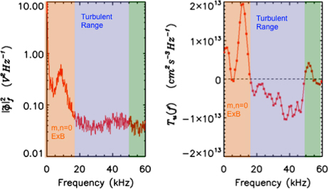
Figure 1. Left: potential fluctuation spectrum showing low-frequency m, n = 0 E × B flow fluctuations (f < 15 kHz) turbulent frequency range (f > 15 kHz). Right: frequency-resolved net kinetic energy transfer. Frequencies between ∼15 and 50 kHz are losing energy to both higher frequencies (f > 50 kHz) and low frequencies (f < 15 kHz) associated with m, n = 0 sheared E × B flows. The error bars on the kinetic energy transfer are estimated from the number of ensembles (N = 300) to be ±0.2 × 10¹³ (cm2 s−3 Hz−1), consistent with the scatter in (b).
Download figure:
Standard image High-resolution imageAdditional insight into this physics can be obtained by considering radial profiles of the Reynolds force
 , the low-frequency E × B flow
 and the product of these two, PRe, which is equal to the rate of work done by the turbulence on the low-frequency E × B flow which in a 0D model satisfies PRe = PLF. The Reynolds stress is computed using a time-domain high-pass digital filter to isolate velocity fluctuations with f > 20 kHz; the product of these fluctuations is then time averaged to produce the
 (figure 2 left panel). The low-frequency E × B shear flow is computed from the radial gradient of the time-averaged plasma potential (figure 2 centre panel) and PRe is then computed from the product of the first two results (figure 2 right panel). We show results for ohmic (black curves) 380 kW ECH (blue curves) and 730 kW ECH (read curves) heated discharges. The results clearly show that in these time stationary L-mode discharges the Reynolds force acts to reinforce the E × B flow, and as a result the turbulence transfers energy into the large-scale shear flow consistent with the model expectations for fixed-point L-mode behaviour. Furthermore, the Reynolds force, the magnitude of the shear flow and the production term all increase substantially as the heating power is increased. These results show that the turbulence is acting to reinforce or amplify the shear flow at the boundary, and that this effect becomes stronger as the heating power is raised. The predator–prey model would then predict that when the transfer rate exceeds γZF, then
can grow to much larger amplitudes and extract a significant fraction of energy from the turbulence. Without the knowledge of this damping rate, we cannot test this prediction in the HL-2A data. However, experiments in DIII-D (discussed next) do allow us to examine these expectations in a more quantitative manner.
(figure 2 left panel). The low-frequency E × B shear flow is computed from the radial gradient of the time-averaged plasma potential (figure 2 centre panel) and PRe is then computed from the product of the first two results (figure 2 right panel). We show results for ohmic (black curves) 380 kW ECH (blue curves) and 730 kW ECH (read curves) heated discharges. The results clearly show that in these time stationary L-mode discharges the Reynolds force acts to reinforce the E × B flow, and as a result the turbulence transfers energy into the large-scale shear flow consistent with the model expectations for fixed-point L-mode behaviour. Furthermore, the Reynolds force, the magnitude of the shear flow and the production term all increase substantially as the heating power is increased. These results show that the turbulence is acting to reinforce or amplify the shear flow at the boundary, and that this effect becomes stronger as the heating power is raised. The predator–prey model would then predict that when the transfer rate exceeds γZF, then
can grow to much larger amplitudes and extract a significant fraction of energy from the turbulence. Without the knowledge of this damping rate, we cannot test this prediction in the HL-2A data. However, experiments in DIII-D (discussed next) do allow us to examine these expectations in a more quantitative manner.

Figure 2. Profiles of (a) Reynolds force, (b) 〈E〉 × B profiles (middle) and (c) rate of Reynolds work, PRe for ohmic (black), 380 kW ECH heating (blue) and 730 kW ECH heating (red) discharges in HL-2A. Increased ECH heating results in an increased Reynolds force, an increased sheared E × B flow inside the LCFS and an increased PRe which acts to reinforce the E × B flow in the region inside the LCFS.
Download figure:
Standard image High-resolution image3.2. Transition to LCO or I-phase regime
The transition to LCO behaviour is studied in DIII-D LSN discharges. The midplane fast scanning probe is inserted during the L-mode, is stationary approximately 1 cm inside the LCFS while it captures the L–I transition, and then is retracted in the early (∼10 ms) I-phase. The resulting time-resolved measurements just inside the LCFS (figure 3) then permit us to study the evolution of the power transfer into the m, n = 0 shear flow during the onset of the LCO regime. The results show that
begins to increase slightly (a few hundred µs) before the oscillations in divertor Da light (which are characteristic of the LCO regime) begin (figures 3(a) and (b)). The time required for parallel plasma propagation along the field lines can introduce a slight (∼100–200 µs) delay between the
oscillations and the divertor Da light oscillations, and thus this slight delay may reflect the time needed for parallel transport processes to begin to modulate plasma particle input into the divertor due to modulations of cross-field transport. A comparison of the rate of energy transfer,
 and the plasma-frame turbulent decorrelation rate
provides important insights into the physics of the onset of the LCO or I-phase regime. Here the ratio
provides a measure of the effective rate of energy transfer from the turbulent frequency range into the m, n = 0 shear flow. The rate
is computed from the measured laboratory frame decorrelation rate γdecorr|lab, the measured poloidal decorrelation length
and the plasma-frame turbulent decorrelation rate
provides important insights into the physics of the onset of the LCO or I-phase regime. Here the ratio
provides a measure of the effective rate of energy transfer from the turbulent frequency range into the m, n = 0 shear flow. The rate
is computed from the measured laboratory frame decorrelation rate γdecorr|lab, the measured poloidal decorrelation length
 and the measured low-frequency E × B drift velocity
via the relation
and the measured low-frequency E × B drift velocity
via the relation
 . The results (figure 3 lower panel) show that in the fixed-point L-mode regime, just before the transition to LCO regime, the turbulence has
 , indicating that turbulent energy is dissipated to both LF E × B flows and to high frequency, high wavenumber (and thus presumably viscous) dissipation processes at comparable rates. Furthermore, because the L-mode state is time stationary, we can estimate that in L-mode just prior to entry into the LCO regime, the net rate of energy input into the turbulence must balance these combined dissipation processes, and thus we can estimate the effective energy input rate in L-mode as
 . Examining the magnitudes of the stress and E × B flow in L-mode, we can also estimate γZF ∼ 105 s−1.
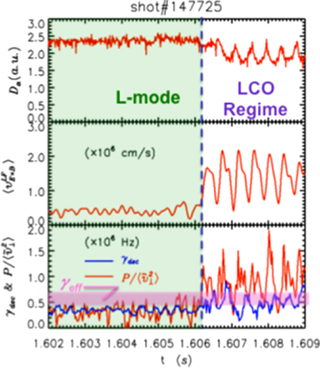
Figure 3. Top: Da light modulations. Middle: m, n = 0 E × B flow velocity. Bottom: plasma frame decorrelation rate (blue) and rate of energy transfer into m, n = 0 E × B flow,
 (red). Energy transfer into m, n = 0 E × B flows becomes the dominant turbulent energy loss channel in the LCO regime. Data obtained 1 cm inside DIII-D LCFS.
Download figure:
Standard image High-resolution imageThe transition to the LCO state is observed to occur at about 1.6062 s as seen by the onset of oscillations in the data in figure 3. In the short (a few hundered µs) time period of the onset of the LCO phase, it seems unlikely that the mean density and temperature profiles would be able to evolve. Thus, the free energy source driving the turbulence and the (m, n = 0) flow-damping rate γLF will remain roughly constant across the transition into the LCO state. Examining the results in figure 3(c), we note that at the onset of the LCO regime, the
 channel increases by a factor of ∼2–3 to a value of about 106 s−1 or so at 1.606 s while the decorrelation rate shows no similar prompt jump. Clearly then
becomes the dominant turbulent energy dissipation channel as the LCO regime is entered. As a result, changes in
can have a significant impact on the turbulent energy balance via the model equations given above.
channel increases by a factor of ∼2–3 to a value of about 106 s−1 or so at 1.606 s while the decorrelation rate shows no similar prompt jump. Clearly then
becomes the dominant turbulent energy dissipation channel as the LCO regime is entered. As a result, changes in
can have a significant impact on the turbulent energy balance via the model equations given above.
3.3. Direct evidence that turbulent stress drives the m, n = 0 sheared E × B flow
The above results are consistent with an interpretation that the time-varying shear flow in the LCO regime is in fact driven by the turbulence. Further supporting evidence can be found by an examination of the time-variation of the turbulent stress, turbulent energy and E × B shear flow during the LCO phase. Figure 4 presents a detailed examination of these quantities obtained from probe measurements taken ∼1 cm inside the LCFS during a DIII-D LCO discharge. The stress and turbulent energy both grow as the m, n = 0 E × B flow approaches its minimum value. Then, as the stress reaches its most negative value, the m, n = 0 E × B flow begins to accelerate and reaches its maximum acceleration either just at or very shortly after the peak in the turbulent stress. Since the stress is nearly zero outside the LCFS, we can take the Reynolds force as being proportional to the value of the stress; thus stress modulation represents a Reynolds force modulation. We therefore conclude that the stress can provide an acceleration which then modulates the m, n = 0 E × B flow and that the observed flow dynamics are consistent with this interpretation.
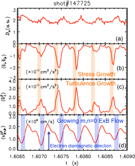
Figure 4. (a) Da light modulations, (b) turbulent stress and (c) turbulent energy, (d) m, n = 0 E × B flow velocity. Data taken ∼1 cm inside LCFS in DIII-D LCO regime.
Download figure:
Standard image High-resolution imageWe have also used BES turbulence imaging to study the power transfer evolution during the same L-mode to LCO transition. In particular, we have used velocimetry analysis [11, 12] of BES imaging data obtained in the same discharges to provide a similar calculation of the shearing rate and nonlinear power transfer rate during the L-mode to LCO transition. The results (figure 5) provide a qualitatively similar picture of the onset of strong nonlinear power transfer into the low-frequency shear flow at the moment of the LCO transition, and a subsequent modulation in this transfer rate during the LCO regime. Thus, these results do not seem to depend upon the use of probes to infer the results. We also note that radially resolved probe measurements show that these effects are localized to the region slightly (<1 cm) inside the LCFS (figure 6).

Figure 5. Nonlinear kinetic energy transfer rate during the transition from L-mode to the LCO regime. Data obtained by velocimetry analysis of DIII-D BES turbulence imaging data of DIII-D shot 147725, centred on region 1 cm inside the LCFS. The results show a jump in the relative rate of nonlinear energy transfer to the low frequency m, n = 0 sheared E × B flow at ∼1606.3 ms and then a subsequent modulation in this transfer rate during the LCO regime, in qualitative agreement with probe results.
Download figure:
Standard image High-resolution image
Figure 6. Top: radial profiles of low frequency E × B drift profiles in L-mode (blue), I-phase or LCO regime (red) and H-mode (green). Bottom: radial profiles of normalized energy transfer rate
into the m, n = 0 E × B flow in L-mode (blue), LCO or I-phase (red) and H-mode (green), and estimated range of γeff from the preceding L-mode phase of the discharge (pink band).
Download figure:
Standard image High-resolution image3.4. LCO to H-mode transition
The radial profiles of
and
 obtained in L-mode, in early LCO phase, and in early (∼10 ms after onset) H-mode are shown in figure 6. The mean E × B velocity profile shows a weak shear layer in L-mode, and periods of significantly stronger flow in the LCO or I-phase regime. In the region inside the LCFS the E × B velocity shows large oscillations in the LCO regime, documented in detail above. In the H-mode, the E × B profile appears to 'lock-in' the peak values of
 and
and
 found in the LCO or I-phase regime. In the LCO or I-phase regime, the transfer rate
 increases markedly from L-mode values, and exhibits large variations as the m, n = 0 E × B flow and turbulence intensity oscillations occur. In H-mode, the power transfer rate then locks into values as large as those found in the intermediate LCO regime and equals or exceeds the L-mode effective energy input rate γeff from the free energy source.
3.5. L–H transition
The above results provide detailed insight into the L-LCO-H mode transition sequence. However, the question remains as to whether or not a similar physics picture is observed in a 'normal' L–H transition that does not exhibit the intermediate LCO phase. We have performed experiments on the EAST device which provide an answer to this question. We used a single discharge that exhibited an L-LCO-H mode transition, went back into L-mode, and then had a normal L–H transition. The macroscopic parameters of the plasma were quite similar during these two transitions, allowing us to use results from the LCO regime in the analysis of the L–H transition. A detailed discussion of these results can be found in a recent paper [13].
Measurements of the rate of turbulence kinetic energy recovery
 made in the LCO regime during periods when the zonal flow magnitude is negligible provide a direct experimental measurement of the net rate of energy input into the turbulence, i.e. of the quantity (γeff − γdecorr) which gives the net rate of energy input into the turbulence after accounting for transfer to high wavenumber scales where viscous dissipation occurs. These data are taken under conditions in which the edge gradients during the LCO regime and the L–H transition are the same to within the uncertainty of the measurements. The plasma in these experiments is therefore sitting very close to the threshold for the transition to improved confinement. Multipoint probe measurements then provide a measure of PLF during a 'normal' L–H transition that does not exhibit an LCO phase but which otherwise has edge plasma gradients are nearly identical to those found during the LCO phase. Because the edge pressure gradients are similar, then presumably the net rate of energy input into the turbulence, γeff − γdecorr is unchanged going from the LCO to the L–H regimes. As a result, we can use the net rate of energy input γeff − γdecorr during the LCO regime to the study of the L–H transition. The ratio
 then indicates the ratio of the power transfer into the ZF normalized by the net power input into the turbulence. Should this value exceed unity, then according to the model described above, the turbulent energy should drop significantly. The experimental results (figure 7) show that this ratio does in fact peak near unity just before or at the drop in Dα, which signifies the entrance into the H-mode regime. Thus, just before an L–H transition the power transfer into the m, n = 0 E × B flow becomes, momentarily at least, strong enough to transfer the turbulence energy to the flow at a rate faster than it can be input from the mean gradients, resulting in an observed turbulence collapse that is consistent with model expectations. Since cross field transport is caused by the turbulence, this collapse then leads to the build-up of the edge gradients and associated mean shear flow. A detailed discussion of these observations and a comparison with predator–prey model results is available in the literature [13].

Figure 7. Top: Da evolution during EAST L–H transitions. Middle: turbulent radial kinetic energy and low-frequency sheared E × B flow energy. Bottom: ratio of production, PLF normalized to the effective rate of energy input into the turbulent scale,
 . Error bars on bottom panel estimated from propagation of random statistical errors. Green line: SOL data. Blue and red: data obtained ∼1 cm inside LCFS.
Download figure:
Standard image High-resolution image
4. Comparison with predator–prey model
There are multiple points of agreement between the experimental observations and the predator–prey model which is the motivation for the power balance model described above. First the turbulence helps to sustain the m, n = 0 E × B flow via a transfer of kinetic energy from the microscopic turbulence scale to the mesoscopic zonal flow scale, and growth of the E × B flow comes at the expense of the turbulent energy—which is an essential element of the predator–prey model. Furthermore this flow drive gets stronger as heating power is raised. Second, the temporal relationship between turbulent stress and the sheared E × B drift is consistent with the model. Third, our experiments taken together with published work are consistent with the energy transfer in early LCO being associated with the turbulence-driven plasma flow, while later in the LCO regime and in H-mode the diamagnetic component of the m, n = 0 E × B flow associated with grad-Pi (a.k.a. the MSF) becomes dominant [6]. Finally, the fast L–H transition appears to be a compressed version of this process in which a transient increase in turbulence-driven sheared E × B flow extracts nearly all the energy from the turbulence, which then collapses [13]. In particular, a detailed discussion of the predator–prey model predictions for both L-LCO-H mode and L–H transitions is also available [9]. Here we point out figure 7 in this last reference, which provides an analogous plot of the evolution of turbulence energy, zonal flow and mean shear flow energy, and nonlinear energy transfer rate during an L–H transition. That result clearly shows the important role that the rate of energy transfer into the turbulent-driven sheared E × B flow (the 'zonal flow' in the parlance of the predator–prey model) plays in initiating the L–H transition. Finally, although the EAST experiments do not yet have the requisite diagnostics, it is already well known that a strongly sheared E × B flow associated with a steep grad-Pion can then develop at the H-mode transition, providing a mechanism to maintain the shear flow once the turbulent flow drive dies away after the onset of H-mode.
5. Summary and conclusions
We find that the rate of Reynolds work done by turbulence on the mesoscale sheared m, n = 0 E × B flows increases substantially as the L-mode heating power is increased due to an increase in the Reynolds force and in
. At the transition to the LCO regime, the rate of energy transfer to the m, n = 0 E × B flows,
, becomes 2–3 times larger than the plasma-frame turbulent decorrelation rate,
, and thus, for a fixed rate of energy input from the free energy source, will effectively govern the turbulence amplitude. This shows that the rate of m, n = 0 flow drive then becomes the dominant turbulent energy sink in the LCO regime. Measurements ∼1 cm inside LCFS show that in the LCO regime, the turbulent kinetic energy
,
and Reynolds stress are strongly modulated in time, and the system can be considered to execute multiple orbits in a
 phase space. The peak Reynolds force is associated with the peak acceleration of
, and increases in
come at the expense of
. We note that during the LCO, the shearing rate of
is nearly equal to and tracks the variation of
, which suggests that the more commonly used shearing rate
could actually be a measure of the rate of power transfer out of the turbulence and into the LF m, n = 0 shear flows. As the LCO progresses, published work [6] shows that the diamagnetic E × B flow associated with ∇pion gradually increases to the point where
phase space. The peak Reynolds force is associated with the peak acceleration of
, and increases in
come at the expense of
. We note that during the LCO, the shearing rate of
is nearly equal to and tracks the variation of
, which suggests that the more commonly used shearing rate
could actually be a measure of the rate of power transfer out of the turbulence and into the LF m, n = 0 shear flows. As the LCO progresses, published work [6] shows that the diamagnetic E × B flow associated with ∇pion gradually increases to the point where
 can maintain turbulence suppression. At the onset of H-mode the LCOs cease and the E × B shearing rate and power transfer lock into the strong flow shear and reduced turbulence and transport. During a rapid (i.e. a 'normal') L–H transition that does not exhibit an LCO regime, the power transfer is observed to transiently extract nearly all of the turbulence energy and transfer it into
, thereby quenching turbulent transport and allowing the steep gradients and mean shear flow associated with H-mode to then develop. These qualitative results compare favourably with a predator–prey model. Interestingly, we note that recent work in ALCATOR C-Mod shows that the Reynolds stress mediated power transfer from the fluctuations into the finite frequency GAMs also plays an important role in the onset of the I-mode [15]. Thus, the nonlinear physics of turbulent-driven shear flows appears to play a key role in the formation of a number of types of improved confinement transitions in many devices.
can maintain turbulence suppression. At the onset of H-mode the LCOs cease and the E × B shearing rate and power transfer lock into the strong flow shear and reduced turbulence and transport. During a rapid (i.e. a 'normal') L–H transition that does not exhibit an LCO regime, the power transfer is observed to transiently extract nearly all of the turbulence energy and transfer it into
, thereby quenching turbulent transport and allowing the steep gradients and mean shear flow associated with H-mode to then develop. These qualitative results compare favourably with a predator–prey model. Interestingly, we note that recent work in ALCATOR C-Mod shows that the Reynolds stress mediated power transfer from the fluctuations into the finite frequency GAMs also plays an important role in the onset of the I-mode [15]. Thus, the nonlinear physics of turbulent-driven shear flows appears to play a key role in the formation of a number of types of improved confinement transitions in many devices.
There are several obvious next steps to take. First, experiments need to directly separate the evolution of the m, n = 0 E × B into the ion pressure gradient and v × B components in order to clearly resolve the role of 'zonal flows' and mean shear flows in this evolution, and a quantitative comparison with the predator–prey model should be done. Second, the understanding from this work should now be used to develop a macroscopic model of the L–H threshold that is based on microscopic physics. Third, we note that three-dimensional effects may be important, motivating measurements of the other components of the turbulent stress matrix as was pointed out earlier by other workers [14]. Such work would then naturally link the L-LCO-H mode transition physics to the physics of intrinsic toroidal rotation. Finally, we note that these physics are essentially hydrodynamic processes, describable with fluid based models of the plasma that properly account for neoclassical flow damping and, perhaps, electromagnetic effects. Thus, we can conclude that the L–H transition physics should be capable of being captured by suitable turbulence-based simulations first using fluid and gyro-fluid models. These could be used to gain deeper insights into the physics that could eventually permit gyrokinetic-based simulations to then reproduce these dynamics.
Acknowledgments
This work was supported by the Natural Science Foundation of China, Project Nos 11175060, 11075046 and 11175056, and by the National Magnetic Confinement Fusion Science Program of China under Contract Nos 2011GB107001 and 2010GB106008; by the US Department of Energy (DOE) through Grant Nos DE-SC0001961, DE-FG02-08ER54984, DE-FG02-89ER53296, DE-FG02-08ER54999, DE-FG02-07ER54917 and DE-FC02-04ER54698; and by the WCI Program of the National Research Foundation of Korea funded by the Ministry of Education, Science and Technology of Korea [WCI 2009-001]. The authors would like to acknowledge the facilities, organizing Committee and participants of the Festival de Theorie, Aix en Provence, 2011 for stimulating discussions which helped motivate this work, and the work of the HL-2A, EAST and DIII-D teams for making these experiments possible.